Abstract
This study develops a two-dimensional (z-x direction) atmospheric dynamics model based on a set of simplified atmospheric motion equations, designed for rapid simulation of atmospheric flow characteristics over complex terrains. The model effectively captures the influence of topography on the atmospheric flow field, offering a new research tool for the in-depth investigation of atmospheric dynamic phenomena under complex terrain conditions. Furthermore, the model takes into account water vapor transport and condensation processes, and employs a simplified algorithm for the conversion of cloud droplets to raindrops to estimate the intensity and spatial distribution of precipitation. The innovative use of the z-coordinate system allows for a focused simulation of dynamic processes in complex terrains, capable of real-time computation of the temporal variations in precipitation processes. The model exhibits high simulation precision and has a wide range of potential practical applications.
1. Introduction
In recent years, significant attention has been devoted to the study of convective precipitation phenomena in complex terrain regions. Particularly in mountainous and valley areas, the distinctive topographical features readily trigger extreme weather events such as thunderstorms and short-duration heavy rainfall [1]. These weather phenomena often lead to geological disasters such as flash floods and debris flows [2]. The underlying cause is the substantial impact of complex terrain on wind flow patterns in these regions [3]. When moisture-laden warm and moist air encounters topographical barriers, it is forced to ascend due to the pushing of air behind and the blocking by the mountainous terrain ahead [4,5]. This ascent results in intense updrafts [6]. Such updrafts facilitate the condensation of water vapor into clouds [7], thereby significantly increasing the probability and intensity of precipitation events [8,9].
Studying weather processes under complex terrain conditions presents significant challenges from model development to validation [10], which are primarily encapsulated in four key aspects. Firstly, the complexity of model mechanisms, which involves the intricate interplay of multiple physical processes [11]. Secondly, the scarcity of empirical data [12], as precipitation events in complex terrains tend to be abrupt and localized [13], making the collection of high-quality empirical data exceptionally difficult [14]. Thirdly, in mountainous and valley regions, small-scale precipitation events occur with high frequency; thus, research often concentrates on these microscale phenomena [15]. Lastly, the triggering and formation mechanisms of precipitation are not yet fully elucidated [16,17], lacking sufficient experimental research and data support [18,19], which poses a considerable challenge in the current research endeavors [20].
Built upon atmospheric dynamics models and incorporating algorithms for water vapor phase transitions and condensation [21,22], a precipitation diagnostic model is constructed. The model takes into account phenomena such as the horizontal movement of air masses, vertical ascent, and convergence of air flows. In terms of the precipitation mechanism, the model comprehensively considers processes including the transport of water vapor, condensation of water vapor, formation of water droplets, and the descent of precipitation particles, aiming to accurately diagnose the precipitation process [23].
Simulating the precipitation process involves modeling the relevant physical processes and effectively integrating these models [24]. This necessitates the development of precise algorithmic models to comprehensively simulate these complex physical processes as fully as possible.
To diagnose precipitation over complex terrain areas, it is necessary to establish a small-scale complex terrain precipitation diagnostic model based on the characteristics of the terrain flow field. The model employs a z-coordinate system in the vertical direction and establishes an Eulerian grid system, where information such as water vapor and liquid water in the air is stored within the grid cells and undergoes material exchange between grid points through fluid transport mechanisms.
Although real atmospheric motion is a three-dimensional process, the substantial workload associated with constructing a three-dimensional model led to the selection of a two-dimensional structure in the experimental design, considering the vertical (z-direction) and horizontal (x-direction) dimensions. Within this framework, a precipitation diagnostic model is introduced to conduct the calculation and analysis of precipitation.
2. Data Description
ERA5 is the fifth-generation global atmospheric reanalysis dataset released by the European Centre for Medium-Range Weather Forecasts (ECMWF). ERA5 provides hourly estimates of a wide range of atmospheric, terrestrial, and oceanic climate variables, with a maximum resolution of 0.25° × 0.25°. The data cover the Earth’s surface on a 30 km grid and utilize 137 vertical levels, ranging from the surface to 80 km, to represent the atmosphere, including uncertainty information for all variables when spatial and temporal resolutions are reduced. ERA5 integrates model data with observational data from across the globe to form a comprehensive and consistent global dataset. The dataset incorporates various sources of observational data, including remote sensing data, ground station measurements, and other data sources. This data assimilation approach enables ERA5 to provide more comprehensive and accurate meteorological information, earning it the designation of ‘reanalysis’ data. The ERA5 dataset includes variables such as temperature, pressure, wind, water vapor content, humidity, and precipitation. ERA5 data accurately reflect the spatiotemporal distribution patterns of local meteorological variables, and its accessibility and global applicability make it widely used in various fields.
3. Dynamic Process Framework
This diagnostic model is built with a fundamental structure and an integrated precipitation diagnostic unit. The fundamental structure performs calculations for atmospheric dynamics, pressure, temperature, and water vapor flux. The precipitation diagnostic unit specifically deals with the calculations of water vapor condensation, the formation of raindrops, and their falling from the clouds.
3.1. Fundamental Formulas
Considering the model’s focus on atmospheric motion over small-scale complex terrain, it is necessary to simplify the equations of motion as much as possible. In this scenario, the effect of the Coriolis force can be disregarded, as it generally becomes significant only over ranges exceeding hundreds of kilometers. In conventional meteorological models, pressure is divided into two components: base pressure and perturbation pressure. The base pressure is used to calculate the mesoscale pressure gradient force, which represents a weak interacting force, while the perturbation pressure is used to simulate the intercompression processes between air masses. In the two-dimensional (z-x) simulation framework, the calculation of the pressure gradient force only needs to consider the variations in perturbation pressure.
Atmospheric Motion: Within the scope of small-scale meteorological models, the movement of air masses is primarily influenced by perturbation pressure. In the vertical direction, the atmosphere maintains a state of hydrostatic equilibrium, where gravity and the pressure gradient force are in balance. Consequently, perturbation pressure becomes the decisive factor affecting vertical motion [25,26].
In this context, λ represents the adaptive coefficient of the grid (in practical calculations, a parameter is required to adjust the proportional relationship between the perturbation pressure δp and the grid spacing), Fx and Fz quantify the frictional forces on air masses in the horizontal and vertical directions, respectively, ρ denotes the density of air mass, g is the acceleration due to gravity, θ is the potential temperature, and θ’ refers to the perturbation potential temperature. (u, w) is the wind speed vector, δp is the perturbation pressure, which is involved in calculating the expansion and compression effects between air masses. qv denotes the water vapor mixing ratio (units: kg/kg), and its variation δqv reflects the increase or decrease in water vapor content; an increase in water vapor leads to a decrease in air density, thereby triggering upward air currents. qc is the cloud droplet mixing ratio, with a positive δqc indicating the condensation of water vapor into cloud droplets; qr represents the raindrop mixing ratio, and a positive δqr indicates the transformation of water vapor and cloud droplets into raindrops. These physical phenomena all influence the vertical velocity of the air.
Perturbation Pressure (δp): Minor fluctuations in atmospheric pressure caused by the movement of air masses, which typically reflect the interactions and dynamic motion states between air masses. The perturbation pressure can also be approximated as follows [27]:
In the above equation, γ denotes the grid adaptive coefficient (in practical calculations, a parameter is required to adjust the proportional relationship between the pressure p and the grid spacing, so that δp can be adapted to the current grid), and δt represents the time step. The equation estimates the degree of compression or expansion experienced by the air mass by analyzing the velocity changes at the grid points surrounding the air mass.
Potential temperature (θ): The temperature reached by an air mass when it rises or descends vertically along its dry adiabatic process [28,29] (i.e., without exchanging heat with the surroundings) to a standard pressure level (usually p0 = 1000 hPa).
where cp represents the specific heat capacity of air, with a value of cp = 1005 J/(kg·K), and R typically denotes the gas constant, which for dry air is 287.15 J/(kg·K).
The form of the perturbation potential temperature variation over time is expressed as follows [30]:
where ρ denotes air density, and κ represents the turbulent diffusion coefficient.
Pressure Equation: This represents the time-dependent changes in pressure across the background grid. The formula for its computation is presented below [31,32]:
In this context, g denotes gravitational acceleration. This formula is applicable for calculating the pressure changes experienced by an air mass during its displacement process.
Utilizing the aforementioned equations, an atmospheric dynamics model was constructed, with its dynamic framework based on the computational strategy outlined in “Applicability Study of Euler–Lagrange Integration Scheme in Constructing Small-Scale Atmospheric Dynamics Models” [33]. The transport processes of water vapor and liquid water were calculated using the semi-Lagrange method.
3.2. Time Step Constraints
To ensure numerical stability, the time step must adhere to the Courant–Friedrichs–Lewy (CFL) condition [34], which states that the product of the time step (δt) and the characteristic velocity should not exceed the spatial step (δx). Therefore, the maximum permissible time step can be expressed as follows:
Herein, lmin represents the minimum value of the grid points, and vmax denotes the maximum speed.
Usually, the grid spacing in atmospheric models is not less than 400 m. In this experiment, the maximum value of the wind vector is restricted to within 10 m/s. Accordingly, the maximum allowable time step can be set to 40 s.
4. The Fundamental Framework of the Precipitation Process
- (I)
- Scheme for Detecting Water Vapor Condensation
Generally, when the water vapor content in the air reaches the saturation vapor pressure, the excess water vapor condenses onto aerosol particles to form minute droplets. The saturation vapor pressure in the air is commonly calculated using the Clausius–Clapeyron equation. The following is an initial description of the computational process [35,36]:
Herein, es represents the saturation vapor pressure of water vapor in the air, with units of pascals (Pa), and Tc denotes the air temperature in degrees Celsius.
Consequently, the saturation specific humidity corresponding to the temperature Tc is given as follows [37]:
Here, qsat denotes the threshold of gaseous water that 1 kg of air can hold, with units of kg/kg. When the water vapor content in the air exceeds the threshold qsat, the excess water vapor will condense into liquid water. In the actual modeling process, the relative humidity threshold is set to RH = 1.05 (this value is chosen as 1.05 instead of 1 to allow for some numerical perturbations during the simulation, providing a certain degree of tolerance in the model). It is assumed that when the water vapor content exceeds 1.05·qsat, the program considers the excess water vapor to condense into liquid water.
Liquid water droplets in the air are categorically divided into two primary types based on their size: cloud droplets and raindrops. Generally, cloud droplets span a diameter range from a few nanometers to about 0.25 mm, while raindrops are defined as having a diameter greater than 0.25 millimeters [38]. Assuming that the condensation of water vapor results in cloud droplets, in the model design, cloud droplets are converted into raindrops according to a certain conversion rate [39].
- (II)
- Conversion of cloud droplets into raindrops
The conversion rate is calculated using a simplified formula [40]:
In the equation, qc and qr represent the water content of cloud droplets and raindrops, respectively, with units in kg/kg.
In the equation, k represents the conversion coefficient, and = 10−3 g/kg denotes a constant.
The raindrop increment Δqr is calculated based on the conversion rate, expressed as follows [41]:
It is assumed that precipitation is triggered when the raindrop content qr in a grid point reaches a certain threshold.
- (III)
- Precipitation determination process
In the model, the gaseous and liquid water content in each grid point is calculated at each time step.
As illustrated in Figure 1, the iterative process for precipitation diagnosis is as follows. Initially, at time step tn−1, water vapor and liquid water (inclusive of cloud droplets and raindrops) are transported within the grid cells along the wind direction. The saturation ratio at each grid point is calculated, and based on this ratio, the contents of water vapor and liquid water within the grid are updated, marking this intermediate time as tn’ (indicating the time between tn−1 and tn). Subsequently, the liquid water content in the grid at tn’ is partitioned into cloud droplets and raindrops based on the ratio of cloud droplet (small water droplets) to raindrop content at tn−1. The contents of cloud droplets and raindrops are then updated according to the conversion rate formula for the aggregation of cloud droplets into raindrops. When the mass of larger raindrops exceeds a certain threshold, it is deemed as precipitation. After accounting for the raindrops that have fallen, the remaining raindrop content at time step tn is obtained.
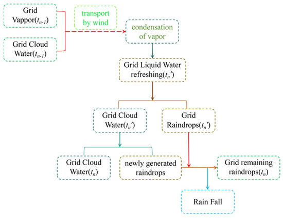
Figure 1.
Iterative computation of the contents of water vapor, liquid water, cloud droplets, and raindrops. Here, tn denotes the time at the nth time step, while tn’ represents the time between tn-1 and tn.
5. Result
5.1. Topographic Wind Field
The case study is situated in the Enshi area of Hubei Province, China, with the precipitation event on 25 September 2018 selected as the research case for analysis.
As shown in Figure 2, Figure 2a illustrates the wind field characteristics at 06:00 on 25 September. Influenced by an outer typhoon, the atmospheric flow field at 850 hPa undergoes dramatic changes, with the region exhibiting an easterly wind pattern. Due to the model’s 2D framework, as depicted in Figure 2b, a z-directional cross-section is selected as the research target within this region. The cross-section corresponds to the red dashed line in Figure 2b. As shown in the figure, the cross-section is aligned parallel to the prevailing wind direction, minimizing disruption from winds perpendicular to the cross-section. Figure 2c illustrates the relative humidity at the 850 hPa height level, revealing that the relative humidity near the target region approaches 100%. Figure 2d displays the water vapor content at the 850 hPa height level (unit: g/kg), indicating that the water vapor content around the target region fluctuates around 10 g/kg.
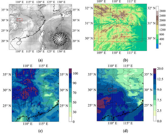
Figure 2.
Weather characteristics of the study area (the red box indicates the study area, and the red curve denotes the selected simulation cross-section). (a) Atmospheric circulation characteristics at 850 hPa; (b) topographical features of the study area; (c) relative humidity of the atmosphere at 850 hPa; (d) moisture content of the atmosphere at 850 hPa.
A 2D atmospheric flow field terrain model was established based on the cross-section corresponding to the red dashed line in Figure 2b. In terms of grid setup, the horizontal grid spacing is 500 m (dx = 500 m), the vertical grid spacing is 100 m (dz = 100 m), and the time integration step is 30 s (dt = 30 s). To observe the model’s sensitivity to actual terrain, a virtual wind field was imported prior to introducing the ERA wind field data.
As shown in Figure 3, the model incorporates real terrain and a simulated wind field, with the simulated wind field set to a horizontal wind speed of −3 m/s. Figure 3a depicts the wind field at the initial moment, while Figure 3b shows the wind field after 10 min of simulation. The filled contour plot represents the horizontal wind speed. Wind vector arrows are displayed at intervals of eight data points along the horizontal direction. As indicated in Figure 3b, the absolute value of the wind speed is greater than 3 m/s over the mountain ridge, whereas in the valley area, the wind speed is significantly reduced. This simulation result aligns with actual observations.

Figure 3.
Simulated terrain and wind field, with filled contours representing the initial horizontal wind speed values. (a) Initial virtual wind field; (b) wind field simulated by the model after 10 min.
As shown in Figure 4, it can be observed from Figure 4a,b that the model exhibits good stability over time. Furthermore, the figures illustrate that on the windward slope, the airflow ascends along the slope, while on the leeward slope, the airflow descends. These results indicate that the wind field simulated by the model conforms to the laws of real atmospheric motion.

Figure 4.
Simulated topographic wind field by the model based on the virtual wind field, with filled contours representing vertical wind speed values. (a) Wind field simulated by the model after 10 min; (b) wind field simulated by the model after 20 min.
Key meteorological data such as wind vectors, air temperature, pressure, and humidity were extracted from the ERA (European Centre for Medium-Range Weather Forecasts reanalysis data). After undergoing filtering processes, these data were used to establish corresponding weight relationships and were interpolated onto the grid system of the diagnostic model.
Simulate the changes in weather conditions from 0 to 59 min. Initially, we will analyze and present the wind field characteristics under the influence of terrain.
As depicted in Figure 5, the filled contour plots in Figure 5a represent the magnitude of the horizontal wind speed, while those in Figure 5b represent the magnitude of vertical wind speed. It can be observed from the figures that the background wind field is quite strong, with significant wind speeds. The background data obtained through interpolation from ERA data take into account the influence of terrain to some extent; however, due to the spatial resolution limitations of the ERA data itself, the estimation of the terrain is relatively coarse.

Figure 5.
Wind field imported from ERA data. (a) Initial wind vectors and horizontal wind speed (shaded contour plot); (b) initial wind vectors and vertical wind speed (shaded contour plot).
Figure 6 illustrates the temporal evolution of the wind field after the initial background wind field has been processed through the diagnostic model. As seen in Figure 6a, there is no significant change in the horizontal wind speed after the model’s correction. Figure 6b reveals that, influenced by the strong winds at high altitudes, a distinct terrain-induced updraft occurs near the windward slopes. This phenomenon is attributable to a continuous inflow of air from the horizontal direction, which, upon encountering topographical obstacles, is forced to ascend, thereby initiating vertical movement in the air current.

Figure 6.
Wind field after model correction. (a) Wind vectors and horizontal wind speed at the 10 min mark (contour plot); (b) wind vectors and vertical wind speed at the 10 min mark (contour plot).
5.2. Precipitation Process
The transport of water vapor in the atmosphere is influenced by variations in wind speed and direction. Its migration process is a result of the combined effects of the atmospheric flow field, terrain characteristics, and various meteorological factors.
As depicted in Figure 7, water vapor in the air is subject to the driving force of the wind field, which continuously supplies external input. On the other hand, it is impeded by terrain features. The transport of water vapor is restricted by high mountains, forcing it to ascend along the mountain slopes.
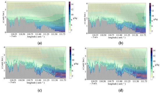
Figure 7.
Temporal variation in the wind field and specific humidity qv (water vapor mixing ratio, unit: g/kg). (a) State at time 0; (b) state at 10 min; (c) state at 20 min; (d) state at 30 min.
Following the attainment of saturation, water vapor condenses into small raindrops.
Figure 8 illustrates the variation in cloud water mixing ratio (qc, where qc denotes the mass of cloud droplets per unit mass of air, unit: g/kg) over time. Panel (a) shows that at 15 min, a cloud mass forms over the mountain, which then rapidly intensifies with time; panel (b) reveals that by 20 min, the water content within the cloud mass has significantly increased; panel (c) indicates that as the transport of water vapor continues, a cloud mass forms over a canyon near 111° longitude at 30 min; and panel (d) demonstrates that at 50 min, the water content of the cloud mass over the canyon near 111° longitude has increased substantially.
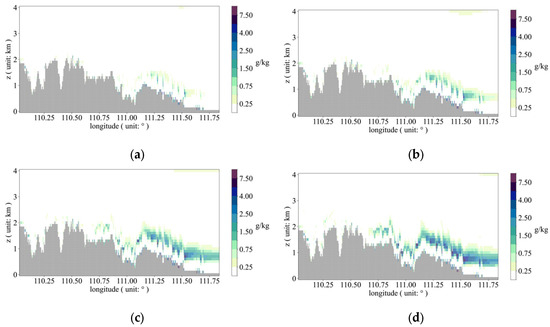
Figure 8.
Temporal variation in cloud droplet water content qc (cloud water mixing ratio, unit: g/kg). (a) State at 15 min; (b) state at 20 min; (c) state at 30 min; (d) state at 50 min.
Figure 9 depicts the temporal evolution of the rainwater mixing ratio (qr, unit: g/kg) within a rain cloud cluster. Figure 9a indicates that at the 20 min time point, the rain cloud cluster emerges above the mountain, after which the mass of raindrops increases progressively and rapidly over time. Figure 9b shows an increase in raindrop mass at the 20 min mark. Figure 9c,d demonstrate that the mass of raindrops reaches a stable condition.
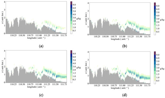
Figure 9.
Variation in rainwater content (rainwater mixing ratio, unit: g/kg) in the rain cloud cluster with time. Panel (a) Status at 20 min; panel (b) status at 30 min; panel (c) status at 40 min; panel (d) status at 50 min.
In the precipitation cloud cluster, raindrops fall to the ground and produce rainfall once they reach a certain mass. The experiment involves measuring the mass of the falling raindrops and converting this measurement into the equivalent precipitation depth upon impact, expressed in millimeters (mm).
Figure 10 illustrates raindrops falling from high altitudes, which contribute to surface precipitation. Figure 10a shows that sporadic precipitation occurs at high altitudes. Figure 10b indicates an increase in the intensity and extent of the precipitation. Figure 10c reveals that the precipitation extends to the vicinity of the canyon above longitude 111°. Figure 10d demonstrates that the intensity of the precipitation remains constant.
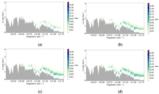
Figure 10.
Precipitation amounts triggered by the model. Panel (a) status at 20 min; panel (b) status at 30 min; panel (c) status at 40 min; panel (d) status at 50 min.
Figure 11 presents the spatial total precipitation amount triggered within one hour, as shown in Figure 11a. Figure 11b displays the cumulative precipitation curve (model result) as output by the model. Due to the high volatility of the curve, a smoothing process is applied to obtain the smoothed precipitation curve (model smooth). Figure 11c employs the results from the smoothed precipitation curve (model smooth) and compares them with ERA precipitation data. It can be observed from the figure that both datasets exhibit a similar trend in precipitation, although there are some discrepancies in the details of the rainfall events.
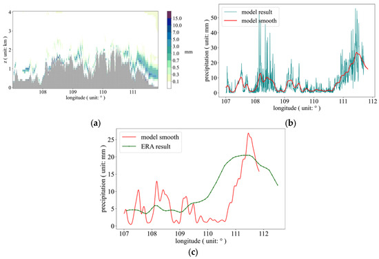
Figure 11.
Panel (a) spatial distribution of the total precipitation triggered by the model over a 1 h period; panel (b) accumulated precipitation over 1 h from the model (model result) and the smoothed model output (model smooth); panel (c) smoothed curve of the 1 h accumulated precipitation from the model (model smooth) compared to the ERA precipitation results.
6. Discussion
The existing meteorological models are generally adequate for routine weather forecasting tasks but have limitations when applied to specific scenarios, such as river basin flood forecasting and short-term predictions in complex terrain regions. Typically, mainstream mesoscale meteorological models (e.g., WRF) require a certain “spin-up time” before they can provide reliable forecast results. This time is usually at least 3 to 6 h, which restricts the real-time forecasting capability of these models in the event of sudden meteorological phenomena. Moreover, river basin flood forecasting heavily relies on high-resolution precipitation predictions. However, due to architectural constraints, current mesoscale models show diminishing improvements when increasing grid resolution below 3 km. Specifically, in the case of the WRF model, terrain data at mesoscale resolution are typically interpolated onto the model grid for simulations and forecasts, rather than using high-resolution terrain data directly. When WRF directly incorporates high-resolution terrain data (e.g., grid sizes below 3 km), it may result in numerical instability, leading to potential model interruptions during operation.
Radar extrapolation models offer unique advantages in short-term forecasting, particularly in flat areas. However, their effectiveness significantly diminishes in complex terrain regions, such as mountains and canyons. Therefore, it is essential to develop rapid precipitation forecasting models tailored to complex terrain to supplement radar-based predictions. Additionally, the development of small-scale meteorological models that are both high-resolution and capable of rapid response is crucial to enhancing short-term forecasting accuracy.
The precipitation diagnostic model used in the experiment calculates a precipitation amount that is generally in agreement with the ERA precipitation trends, albeit with some deviation. The discrepancies between the two are attributed to several factors. On one hand, there is a significant difference in spatial resolution between the two, with the model having a resolution of 500 m grid spacing, whereas the ERA resolution is 0.25° (approximately 30 km). On the other hand, the model is a 2D cross-sectional model, whereas weather processes are three-dimensional, leading to inadequate consideration of certain precipitation factors in the model.
The experimental results presented above suggest that the modeling approach proposed in this paper for complex terrain conditions is feasible. Subsequent efforts should focus on developing the model into a 3D version based on the existing theoretical framework, to be used for precipitation diagnostics in complex terrain settings.
In the context of application, subsequent research should integrate established cloud microphysics schemes into the model. These schemes are models based on physical processes that can accurately depict the formation, growth, coalescence, and dissipation of microphysical particles such as cloud droplets and ice crystals. The incorporation of these mature schemes will offer a more precise foundation for precipitation forecasting.
Additionally, integrating radar data for precipitation diagnosis is an indispensable component in subsequent research. Radar data are characterized by their high spatiotemporal resolution, enabling real-time monitoring of the dynamic changes in precipitation systems. By assimilating radar data into the model and conducting comparative analysis of the simulation results, we can effectively diagnose the strengths and weaknesses of the model, thereby facilitating optimization and refinement of the model.
7. Conclusions
This study integrates fundamental atmospheric principles within an atmospheric dynamics model framework to develop a water vapor transport and condensation model. It simulates the physical processes of water vapor transport and condensation in complex terrains. Furthermore, it introduces a simplified model for cloud droplet to raindrop conversion. By categorizing liquid water in the atmosphere into cloud droplets and raindrops, the model framework efficiently estimates their distribution and enables rapid computation of surface precipitation amounts. The following conclusions were drawn from the study:
- (1)
- The z-coordinate-based motion model possesses unique advantages in simulating atmospheric motion over complex terrain, effectively capturing the movement characteristics that align with real atmospheric conditions.
- (2)
- In this study, a two-dimensional structural design was adopted for the model, with the objective of assessing the applicability of this technology in the construction of weather system models. To improve the model’s ability to simulate complex atmospheric flow fields, future efforts will concentrate on developing a three-dimensional dynamic framework. In addressing small-scale weather processes, the model involved a suitable simplification of the dynamic equations. In subsequent research, the model will incorporate key factors such as pressure gradient force and Coriolis force to more effectively simulate and interpret complex weather phenomena.
- (3)
- The atmospheric model based on the z-coordinate system offers distinct advantages in precipitation simulation for specific application scenarios, particularly in the lower atmosphere. It is especially effective in addressing challenges posed by complex terrain and urban topographic conditions in meteorological simulations.
Author Contributions
Methodology, X.W.; Software, X.W.; Formal analysis, X.W.; Resources, Y.L.; Visualization, C.C.; Data curation, X.C.; Writing—original draft, X.W.; Writing—review and editing, C.C. and J.G.; Visualization, X.C.; Project administration, Y.L. All authors have read and agreed to the published version of the manuscript.
Funding
This research was funded by Project U2340211 supported by National Natural Science Foundation of China (Grant NO.: U2340211), The National Key R&D Program of China (Grant NO.: 2022YFC3002704), The National Key R&D Program of China (Grant NO.: 2023YFC3209105), and the Strategic Consulting Project supported by the Chinese Academy of Engineering (CAE) (Grant NO.: HB2024C18). Special thanks are extended to the editors and anonymous reviewers for their constructive comments.
Institutional Review Board Statement
Not applicable.
Informed Consent Statement
Not applicable.
Data Availability Statement
Additional data associated with this article can be found at https://figshare.com/s/e750c2829d36e96e53c6, accessed on 1 March 2020.
Conflicts of Interest
The authors declare no conflict of interest.
References
- Loginov, V.F.; Volchek, A.A.; Shelest, T.A. Analysis and Simulation of Rain Flood Hydrographs in Belarus Rivers. Water Resour. 2015, 42, 292–301. [Google Scholar] [CrossRef]
- Morell, D.A.; Pereira Filho, A.J.; Beltrán, R.P. Quantitative Rainfall Estimation with a Mobile XPOL Weather Radar. Pure Appl. Geophys. 2022, 179, 2957–2968. [Google Scholar] [CrossRef]
- Dong, W.; Fritts, D.C.; Hickey, M.P.; Liu, A.Z.; Lund, T.S.; Zhang, S.; Yan, Y.; Yang, F. Modeling Studies of Gravity Wave Dynamics in Highly Structured Environments: Reflection, Trapping, Instability, Momentum Transport, Secondary Gravity Waves, and Induced Flow Responses. J. Geophys. Res. Atmos. 2022, 127, e2021JD035894. [Google Scholar] [CrossRef]
- Ikeda, T.; Onaga, H.; Sakurai, Y. Influence of surrounsding weather on the prevention of vapssor condensation and vapor condensation damage by using hygroscopic materials in dwellings: Understanding on properties of moisture content in porous materials and its estimation by condition of cons. J. Archit. Plan. 2000, 65, 9–16. [Google Scholar] [CrossRef][Green Version]
- Takayabu, Y.N. Large-Scale Cloud Disturbances Associated with Equatorial Waves. J. Meteorol. Soc. Jpn. Ser. II 2009, 72, 433–449. [Google Scholar] [CrossRef]
- Wei, X.; Liu, Y.; Chang, X.; Guo, J.; Li, H. Numerical Simulation of Terrain-Adaptive Wind Field Model Under Complex Terrain Conditions. Water 2024, 16, 2138. [Google Scholar] [CrossRef]
- Merritt, G.E.; Weatherston, R.C. Condensation of mercury vapor and drop growth processes in a nitrogen flow. Aiaa J. 2015, 5, 721–728. [Google Scholar] [CrossRef]
- Zhou, Y.; Wang, S.; Fang, J. Diurnal Cycle Dipolar Pattern of Precipitation Over Borneo During the MJO: Linear Theory Nonlinear Sensitivity Experiments. J. Geophys. Res. Atmos. 2023, 128, 2022JD037616. [Google Scholar] [CrossRef]
- Miao, J.E.; Yang, M.J. Amodeling study of the severe afternoon thunderstorm event at Taipei on 14 June 2015: The roles of Sea Breeze microphysics terrain. J. Meteorol. Soc. Jpn. 2020, 98, 129–152. [Google Scholar] [CrossRef]
- Turner, R.; Mcconney, P.; Monnereau, I. Climate Change Adaptation and Extreme Weather in the Small-Scale Fisheries of Dominica. Coast. Manag. 2020, 48, 436–455. [Google Scholar] [CrossRef]
- Hiraga, Y.; Meza, J. Extreme precipitation modeling Probable Maximum Precipitation (PMP) estimation in Chile. J. Hydrol. Reg. Stud. 2025, 58, 102274. [Google Scholar] [CrossRef]
- Wang, H.; Li, Z.; Zhang, T.; Chen, Q.; Guo, X.; Zeng, Q.; Xiang, J. Downscaling of GPM satellite precipitation products based on machine learning method in complex terrain and limited observation area. Adv. Space Res. 2023, 72, 2226–2244. [Google Scholar] [CrossRef]
- Gai, Y.; Long, X.; Wei, Z.; Sui, X.; Jiang, B.; Chen, X.; Yu, D.; Qin, S.; Cui, Y. Toward a better understanding of uncertainty for satellite precipitation products over complex terrain with sparse rain gauge data. Atmos. Res. 2023, 288, 106742. [Google Scholar] [CrossRef]
- Zhang, S.; Solari, G.; De Gaetano, P.; Burlando, M.; Repetto, M.P. A refined analysis of thunderstorm outflow characteristics relevant to the wind loading of structures. Probabil. Eng. Mech. 2017, 54, 9–24. [Google Scholar] [CrossRef]
- Zhang, Y.; Deng, C.; Xu, W.; Zhuang, Y.; Jiang, L.; Jiang, C.; Guan, X.; Wei, J.; Ma, M.; Chen, Y.; et al. Long-term variability of extreme precipitation with WRF model at a complex terrain River Basin. Sci. Rep. 2025, 15, 156. [Google Scholar] [CrossRef] [PubMed]
- Casellas, E.; Bech, J.; Veciana, R.; Pineda, N.; Rigo, T.; Miró, J.R.; Sairouni, A. Surface precipitation phase discrimination in complex terrain. J. Hydrol. 2021, 592, 125780. [Google Scholar] [CrossRef]
- Crochet, P. Enhancing radar estimates of precipitation over complex terrain using information derived from an orographic precipitation model. J. Hydrol. 2009, 377, 417–433. [Google Scholar] [CrossRef]
- Henn, B.; Newman, A.J.; Livneh, B.; Daly, C.; Lundquist, J.D. An assessment of differences in gridded precipitation datasets in complex terrain. J. Hydrol. 2018, 556, 1205–1219. [Google Scholar] [CrossRef]
- de la Fraga, P.; Del-Toro-Guerrero, F.J.; Vivoni, E.R.; Cavazos, T.; Kretzschmar, T. Evaluation of gridded precipitation datasets in mountainous terrains of Northwestern Mexico. J. Hydrol. Reg. Stud. 2024, 56, 102019. [Google Scholar] [CrossRef]
- Zhao, R.; Chen, B.; Zhang, W.; Yang, S.; Xu, X. Formation mechanisms of persistent extreme precipitation events over the eastern periphery of the Tibetan Plateau: Synoptic conditions, moisture transport and the effect of steep terrain. Atmos. Res. 2024, 304, 107341. [Google Scholar] [CrossRef]
- Dheebakaran, G.; Geethalakshmi, V.; Ramanathan, S.P.; Ragunath, K.P.; Kokilavani, S. WRF’s microphysics options on the temporal variation in the accuracy of cluster of village level medium range rainfall forecast in Tamil Nadu. J. Agrometeorol. 2022, 24, 133–137. [Google Scholar] [CrossRef]
- Tiwari, S.; Kar, S.C.; Bhatla, R. Dynamic downscaling over western Himalayas: Impact of cloud microphysics schemes. Atmos. Res. 2018, 201, 1–16. [Google Scholar] [CrossRef]
- Xue, L.; Fan, J.; Lebo, Z.J.; Wu, W.; Morrison, H.; Grabowski, W.W.; Chu, X.; Geresdi, I.; North, K.; Stenz, R.; et al. Idealized Simulations of a Squall Line from the MC3E Field Campaign Applying Three Bin Microphysics Schemes: Dynamic and Thermodynamic Structure. Mon. Weather Rev. 2017, 145, 4789–4812. [Google Scholar] [CrossRef]
- Pflaum, J.C.; Johnson, H.L.; Poellot, M.R. Preliminary Investigations of a Dynamic Seeding Strategy for Oklahoma Convective Clouds. J. Weather. Modif. 1989, 21, 54–61. [Google Scholar]
- Dobashi, Y.; Kusumoto, K.; Nishita, T.; Yamamoto, T. Feedback control of cumuliform cloud formation based on computational fluid dynamics. Acm Trans. Graph. 2008, 27, 1–8. [Google Scholar] [CrossRef]
- Dale, R.D. Improving the anelastic approximation. J. Atmos. Sci. 1989, 46, 1453–1461. [Google Scholar]
- Grell, G.A.; Dudhia, J.; Stauffer, D.R. A description of the fifth-generation Penn State/NCAR Mesoscale Model (MM5). NCAR Tech. Note 1994, 10, 1–121. [Google Scholar] [CrossRef]
- Heymsfield, A.J.; Sabin, R.M. Cirrus Crystal Nucleation by Homogeneous Freezing of Solution Droplets. J. Atmos. Sci. 1989, 46, 2252–2264. [Google Scholar] [CrossRef]
- Rothenberg, D.; Wang, C. Metamodeling of Droplet Activation for Global Climate Models. J. Atmos. Sci. 2016, 73, 1255–1272. [Google Scholar] [CrossRef]
- Garcia-Dorado, I.; Aliaga, D.G.; Bhalachandran, S.; Schmid, P.; Niyogi, D. Fast Weather Simulation for Inverse Procedural Design of 3D Urban Models. Acm Trans. Graph. 2017, 36, 21. [Google Scholar] [CrossRef]
- Çelik, F.; Marwitz, J.D. Droplet Spectra Broadening by Ripening Process. Part I: Roles of Curvature and Salinity of Cloud Droplets. J. Atmos. Sci. 2010, 56, 3091–3105. [Google Scholar] [CrossRef]
- Yang, F.; Kollias, P.; Shaw, R.A.; Vogelmann, A.M. Cloud droplet size distribution broadening during diffusional growth: Ripening amplified by deactivation and reactivation. Atmos. Chem. Phys. 2018, 18, 7313–7328. [Google Scholar] [CrossRef]
- Wei, X.; Liu, Y.; Guo, J.; Chang, X.; Li, H. Applicability Study of Euler–Lagrange Integration Scheme in Constructing Small-Scale Atmospheric Dynamics Models. Atmosphere 2024, 15, 644. [Google Scholar] [CrossRef]
- Abdi, D.S.; Giraldo, F.X.; Constantinescu, E.M.; Carr, L.E.; Wilcox, L.C.; Warburton, T.C. Acceleration of the implicit-explicit non-hydrostatic unified model of the atmosphere (NUMA) on manycore processors. Int. J. High Perform. Comput. Appl. 2017, 33, 242–267. [Google Scholar] [CrossRef]
- Bolton, D. The Computation of Equivalent Potential Temperature. Mon. Weather Rev. 1980, 108, 1046–1053. [Google Scholar] [CrossRef]
- Wei, X.; Liu, Y.; Chang, X.; Guo, J.; Li, H. Mechanism Study of Two-Dimensional Precipitation Diagnostic Models Within a Dynamic Framework. Atmosphere 2025, 16, 380. [Google Scholar] [CrossRef]
- Schneider, T.; O’Gorman, P.A.; Levine, X.J. Water vapor and the dynamics of climate change. Rev. Geophys. 2010, 48, RG3001. [Google Scholar] [CrossRef]
- Seifert, A.; Beheng, K.D. A double-moment parameterization for simulating autoconversion, accretion and selfcollection. Atmos. Res. 2001, 59, 265–281. [Google Scholar] [CrossRef]
- Nober, F.J.; Graf, H.F. A new convective cloud field model based on principles of self-organisation. Atmos. Chem. Phys. 2004, 4, 3669–3698. [Google Scholar] [CrossRef]
- Berry, E.X. Modification of the warm rain process. In Proceedings of the National Conference on Weather Modification Amer, Albany, NY, USA, 28 April–1 May 1968. [Google Scholar]
- Lebo, Z.J.; Seinfeld, J.H. A continuous spectral aerosol-droplet microphysics model. Atmos. Chem. Phys. Discuss. 2011, 11, 23655–23705. [Google Scholar] [CrossRef]
Disclaimer/Publisher’s Note: The statements, opinions and data contained in all publications are solely those of the individual author(s) and contributor(s) and not of MDPI and/or the editor(s). MDPI and/or the editor(s) disclaim responsibility for any injury to people or property resulting from any ideas, methods, instructions or products referred to in the content. |
© 2025 by the authors. Licensee MDPI, Basel, Switzerland. This article is an open access article distributed under the terms and conditions of the Creative Commons Attribution (CC BY) license (https://creativecommons.org/licenses/by/4.0/).