
Elaboration of Simulated Hyperspectral Calibration Reference over Pseudo-Invariant Calibration Reference


Abstract
1. Introduction
- Uncertainties in surface reflectance characterization, which introduce systematic biases. Since these surfaces are assumed to be invariant, addressing this issue is critical. This paper proposes a new method to improve surface BRF characterization.
- Atmospheric property characterization, which plays a crucial role in calibration accuracy. Various improvements are introduced in this study through the combined use of multiple state-of-the-art datasets.
- The accuracy of RTMs used to generate a RCR, which must be carefully evaluated. Sensitivity analyses indicate that discrepancies among different RTMs range from 0.5% to 3%, depending on the spectral region [14]. The proposed approach utilizes Eradiate, a new generation open-source 3D RTM based on Monte Carlo ray-tracing methods, specifically designed for calibration and validation activities [15]. Eradiate allows, among other functions, a spherical shell geometry, overcoming the plane-parallel atmosphere assumption. Future versions of the model will also include polarization, which is expected to improve the simulations especially at low wavelengths.
- Simulations of hyperspectral observations, which require high spectral fidelity. This study demonstrates that the refined methodology achieves agreement within 3% for most spectral regions, thereby supporting the suitability of PICSs for hyperspectral calibration.
2. Data and Methods
2.1. List of Selected PICS
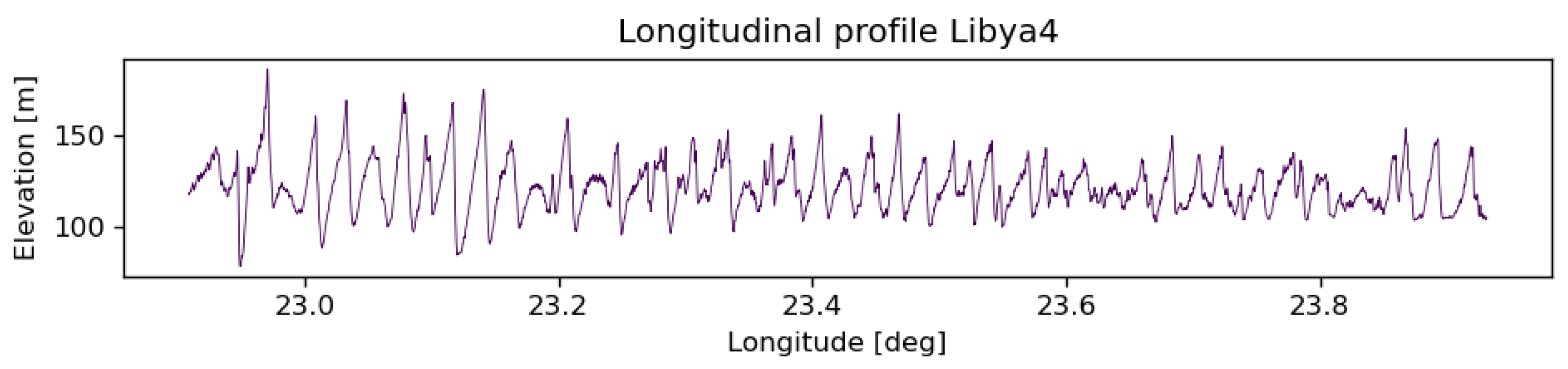
- Libya-4: The most well-known and widely used bright desert PICS, located in the Great Sand Sea. Its significance stems from its large size and radiometric stability, making it essential for radiometer drift monitoring, sensor intercalibration, and absolute calibration based on simulated radiances. Its morphology consists of oriented sand dunes shaped by dominant winds [19]. Some spatial variations in sand granularity are expected depending on dune positioning. Its longitudinal elevation profile is shown in Figure 1.
- Gobabeb: Located in Namibia, this site was added to the list initially proposed in [2]. As part of RadCalNet, it differs from the other sites in having a limited spatial extent of 2 km compared to 20 km for the other targets.
2.2. Surface Reflectance Characterization
2.2.1. Overview of the Approach
- : Governs the mean amplitude of the BRF, predominantly controlling surface albedo.
- k: The modified Minnaert contribution, determining the bowl shape of the BRF.
- : Represents the asymmetry parameter of the modified Henyey–Greenstein phase function.
- : Controls the amplitude of the hot spot due to medium porosity.
2.2.2. Input Data
2.2.3. Atmospheric Effect Removal
2.2.4. RPV Parameter Spectral Interpolation
- Surface BRF simulation. The PICS surface BRF is simulated with the RPV model for all the spectral bands listed in Table 2. The uncertainty associated with these simulated BRF is computed as follows:where and is the correlation between two RPV parameters.
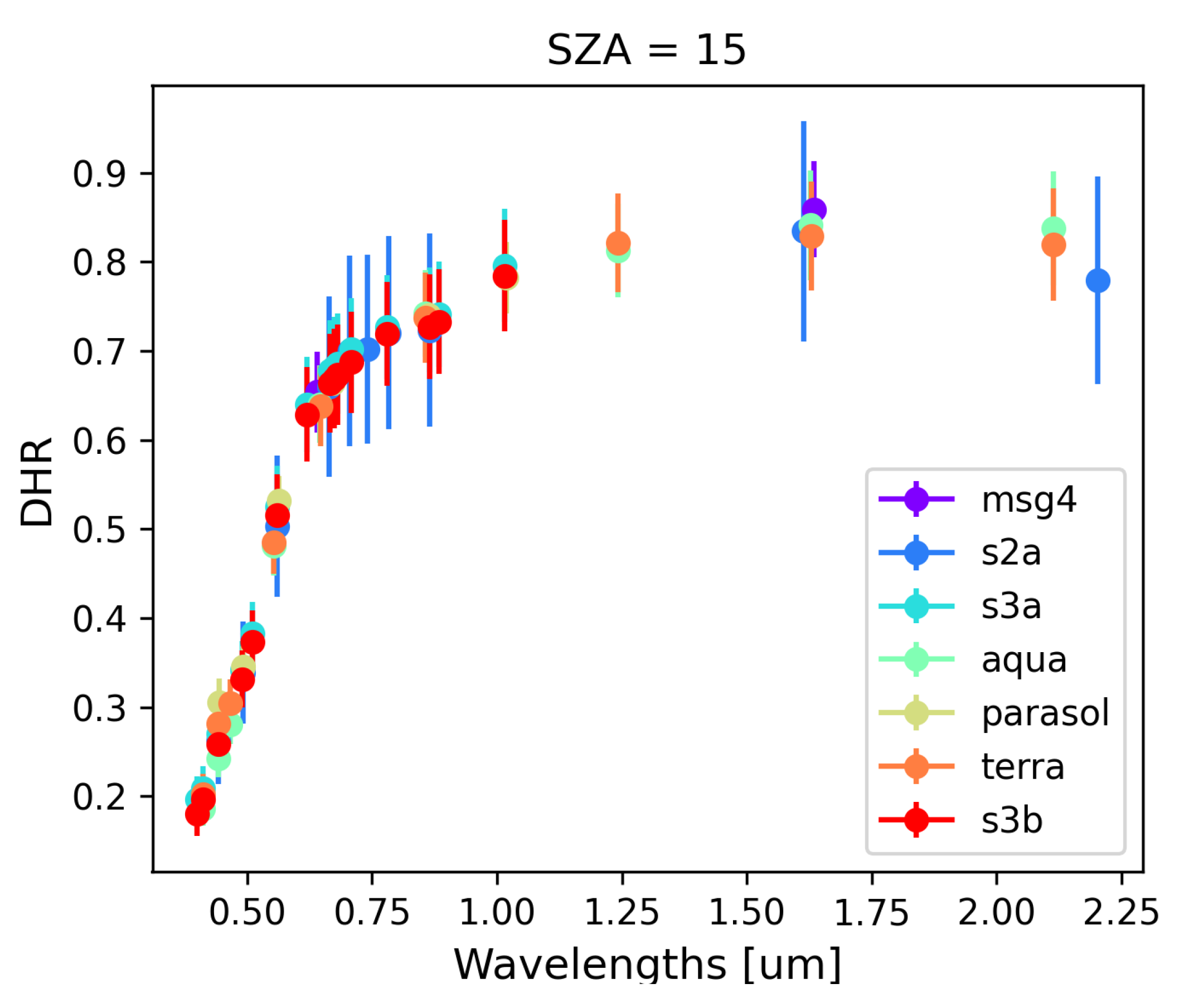
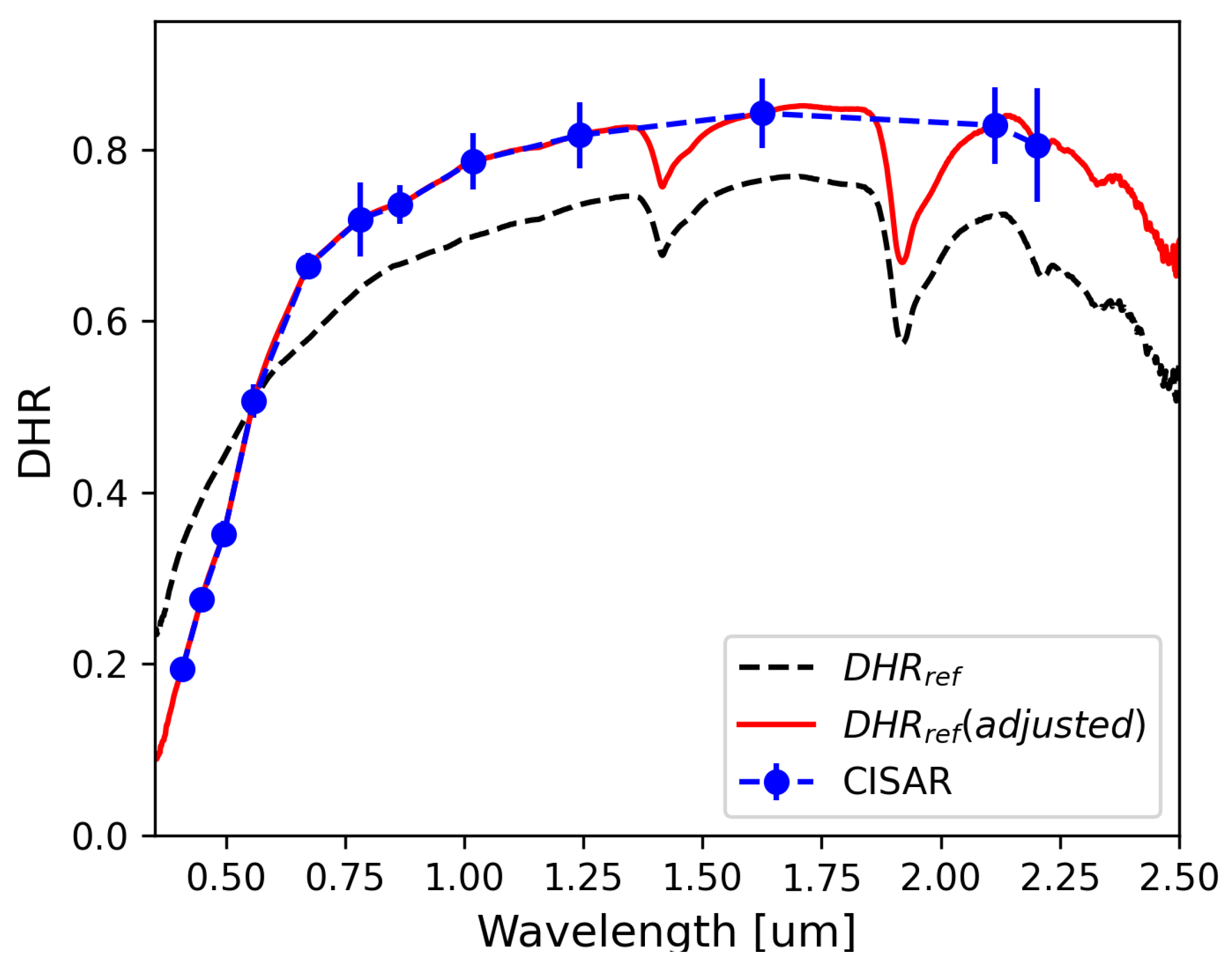
- BRF spectral interpolation. The BRF field simulated in the spectral bands of the selected radiometers is interpolated at a 1 nm resolution from 350 to 2500 nm using the comet_maths tool, developed by National Physical Laboratory (NPL). This tool also returns the interpolated uncertainties and is part of the open-source CoMet Toolkit [26], designed to facilitate the handling of error-covariance information in measurement data analysis. Beyond mathematical calculations for uncertainty propagation, comet_maths incorporates uncertainty-quantified interpolation algorithms. Specifically, it allows to interpolate values between low-resolution data points while preserving the spectral shape of a higher-resolution dataset (or model). The low-resolution data points are computed using the RPV model with parameters retrieved by the CISAR algorithm, while the high-resolution model is derived from the MARMIT database [27], which contains sand optical properties over the 400 nm–2500 nm range. These soil spectra are expressed in terms of DHR [24], with an illumination angle of 15°.To refine the spectral behavior of the DHR, the five best-fitting spectra from the MARMIT database are selected based on minimal Euclidean distance (root-sum-of-squares) to the CISAR retrievals. These spectra are then averaged using a weighting mechanism that accounts for their geometric distance from the CISAR data. The resulting weighted reference curve (dashed black curve in Figure 3, referred to as ) is used by comet_maths to interpolate the spectral behavior of the BRF between the processed wavelengths, incorporating associated uncertainties. This process is illustrated by the red solid line in Figure 3.In addition to interpolation, comet_maths extrapolates the BRF and its uncertainty at the spectral range boundaries, where no CISAR retrievals are available. This extrapolation increases the relative uncertainty of the BRF (defined as the absolute uncertainty divided by the measured value), particularly at shorter wavelengths, where surface reflectance exhibits significant spectral variability.
- Inversion of the high-resolution surface BRF. The third step involves inverting the surface BRF field interpolated at a 1 nm spectral resolution. This process relies on the RPV Model Inversion Package developed in [28], which retrieves the RPV parameters along with the associated covariance matrix. The uncertainty for each parameter corresponds to the diagonal elements of this matrix and tends to be larger at the spectral range extremes due to extrapolation performed by the comet_maths tool.
2.3. Characterization of Atmospheric Properties
2.3.1. Description of the Method
- The fine mode mean radius and standard deviation;
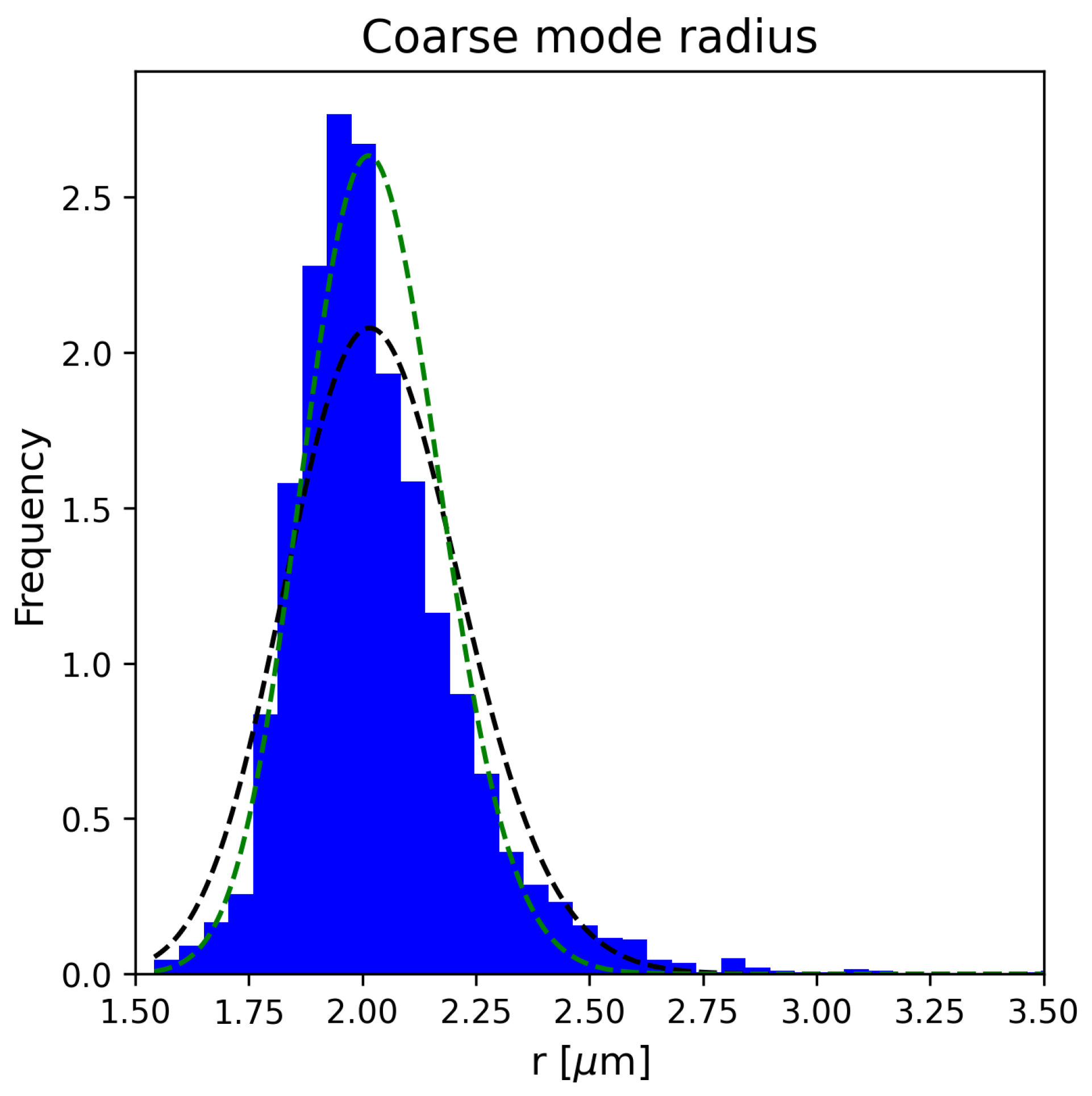
- The coarse mode mean radius and standard deviation;
- The number of particles in each mode;
- The particle oblateness;
- The real and imaginary part of the refractive index.
2.3.2. AERONET Data Analysis
2.3.3. Spectral Interpolation
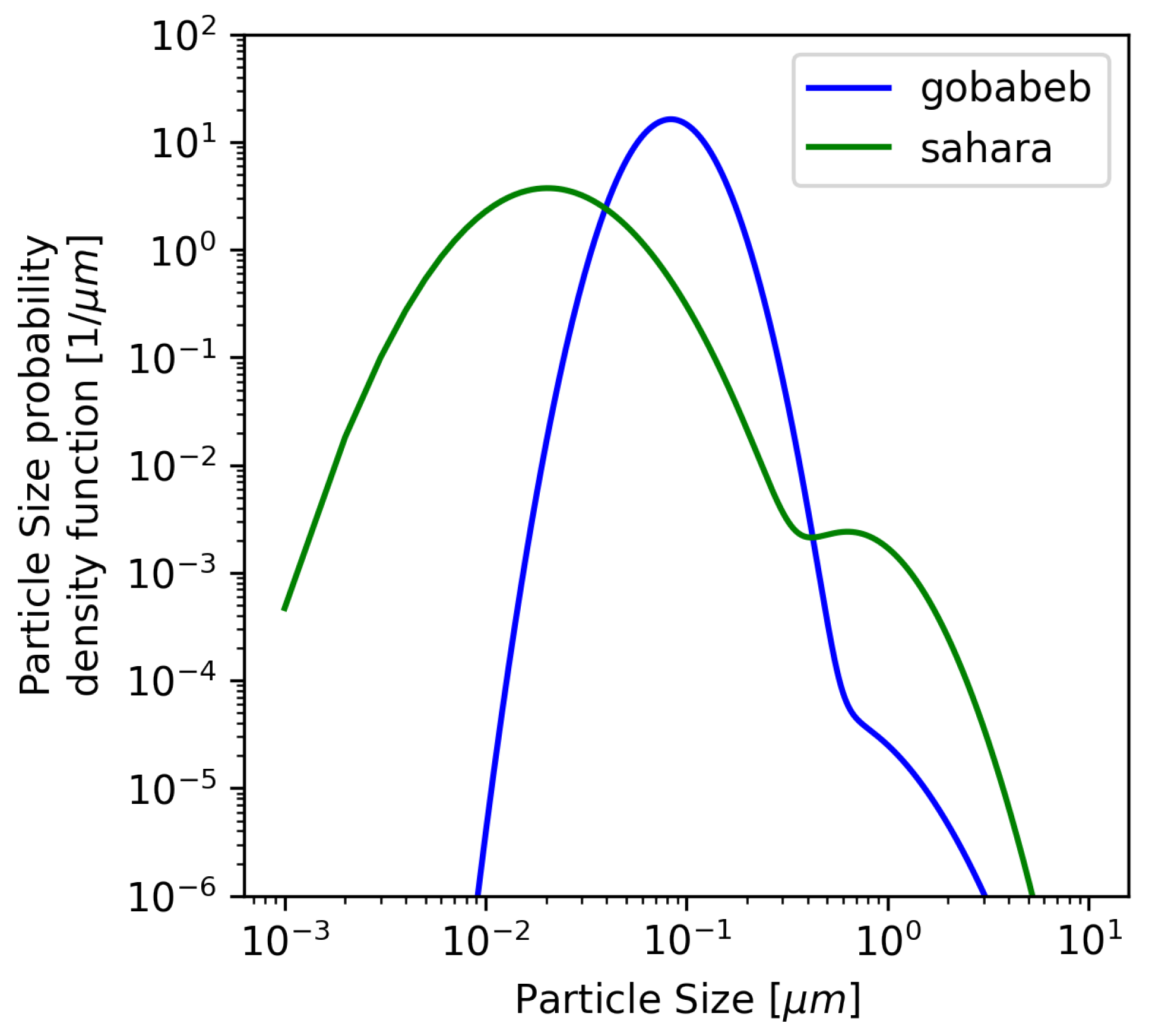
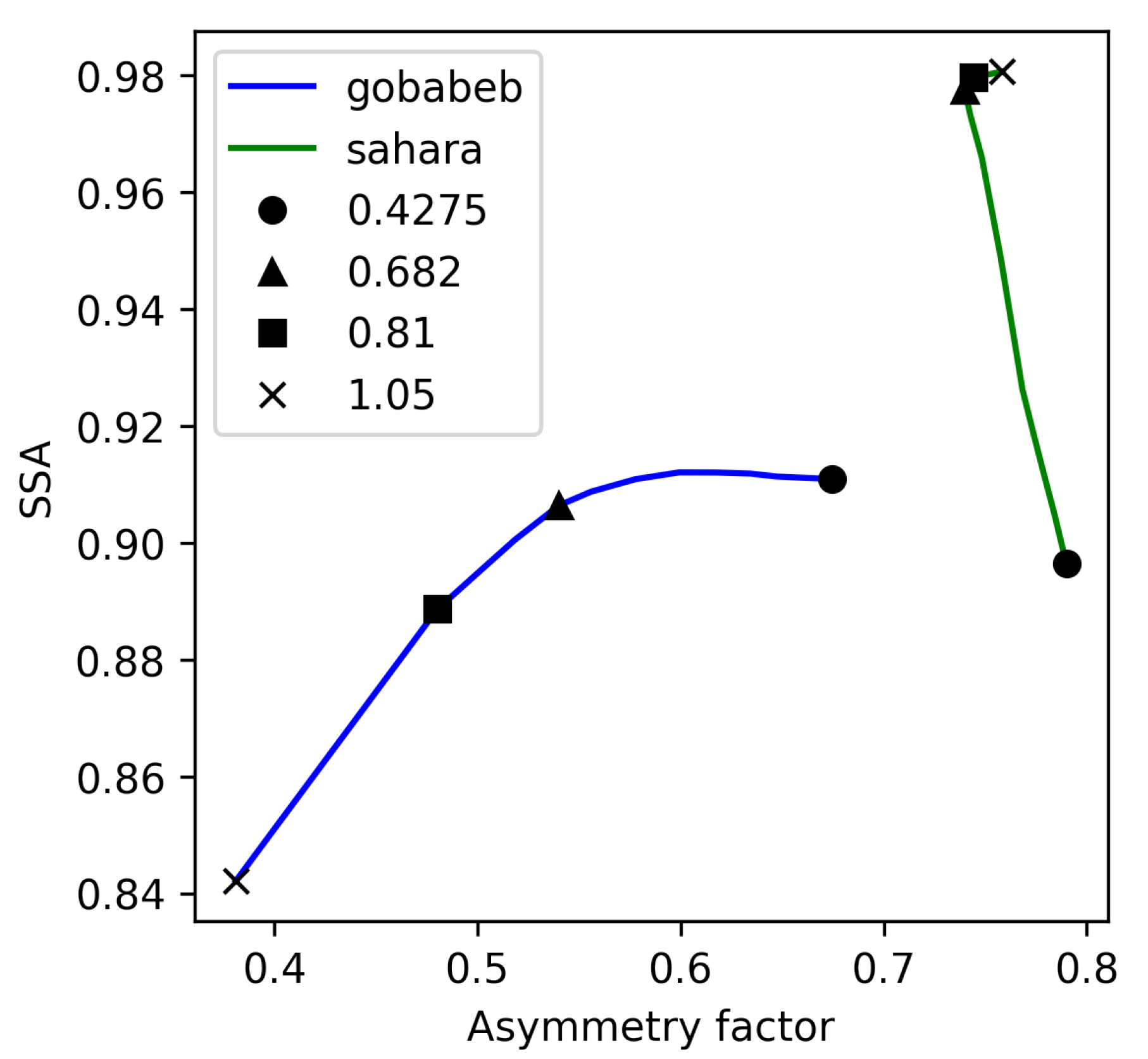
2.3.4. Single Scattering Properties and AOT Estimation
2.4. Calibration Reference Accuracy Analysis
- Fast convergence to a stable bias: few iterations are needed to reach a reliable estimate.
- Reduced uncertainty: the much lower standard deviation compared to [41] implies that the surface anisotropy and atmosphere characterization are improved.
3. Results
3.1. Generation of Calibration Reference
- A flat surface at the elevation given in Table 1, with reflectance characterized using the RPV model.
- A uniform aerosol layer composed of fine and coarse modes, as detailed in Section 2.3.
- The vertical profile of pressure, temperature, and molecular concentrations generated following [33].
- An irradiance dataset expressing exo-atmospheric solar radiation at 1 Astronomical Unit (AU). The Total and Spectral Solar Irradiance Sensor-1 (TSIS-1) Hybrid Solar Reference Spectrum (HSRS) [42] serves as the default model in Eradiate.
- Generation of RCR at 1 nm resolution using Eradiate, producing simulated TOA BRF over selected spectral intervals and viewing geometries , where and represent the illumination and viewing angles.
3.2. Multispectral Results
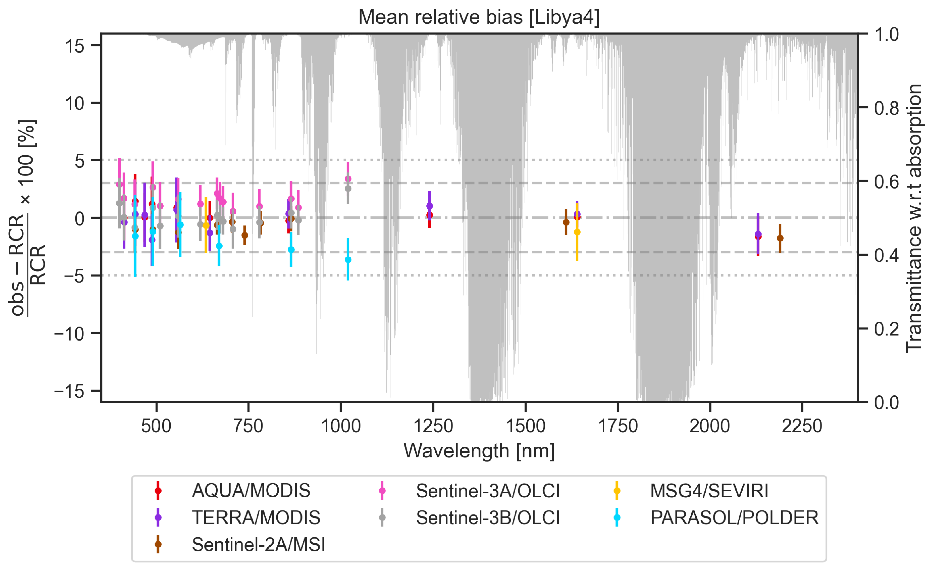
3.2.1. Libya4
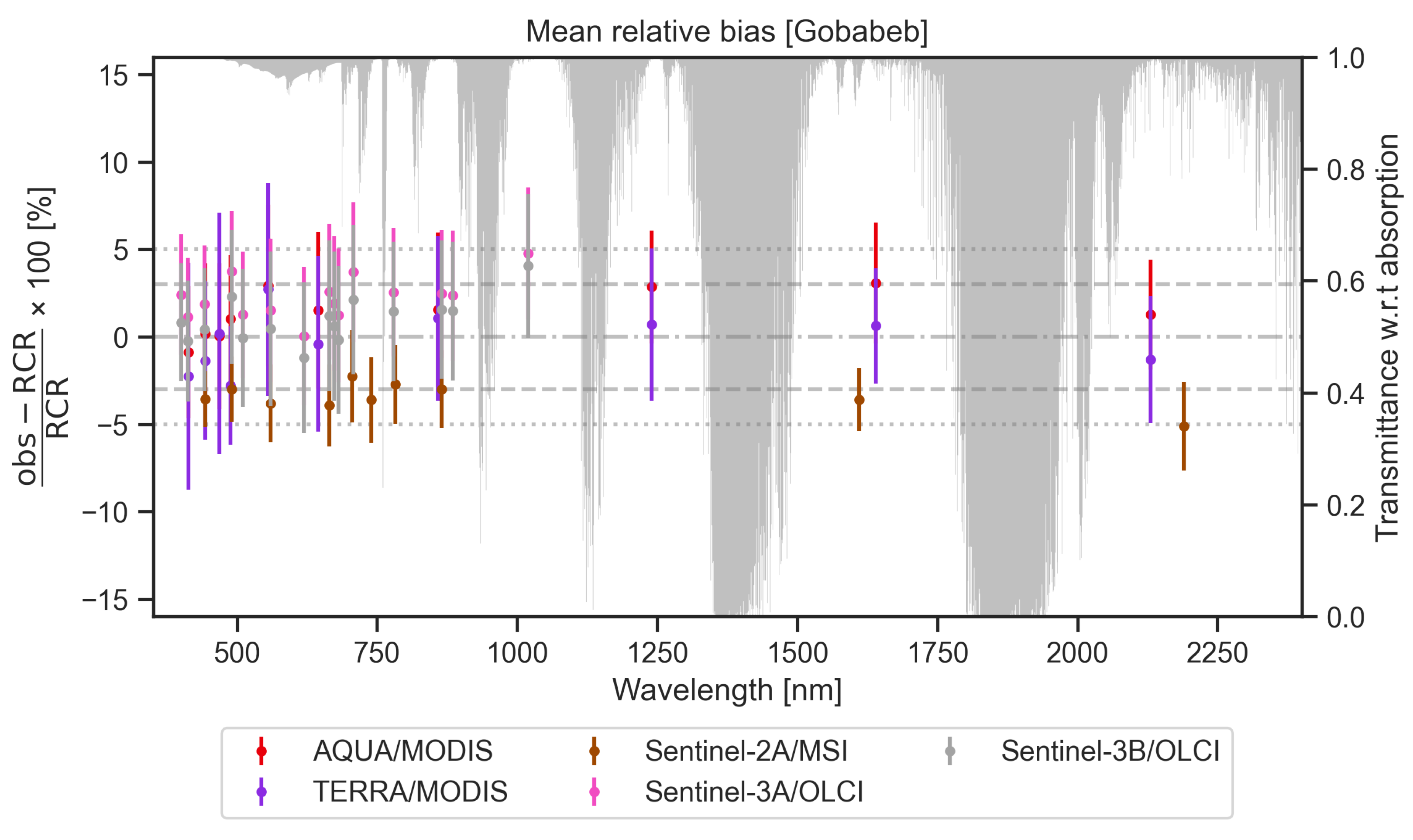
3.2.2. Gobabeb
3.2.3. Performance Assessment of the Simulated RCR with Multispectral Sensors
3.3. Hyperspectral Results
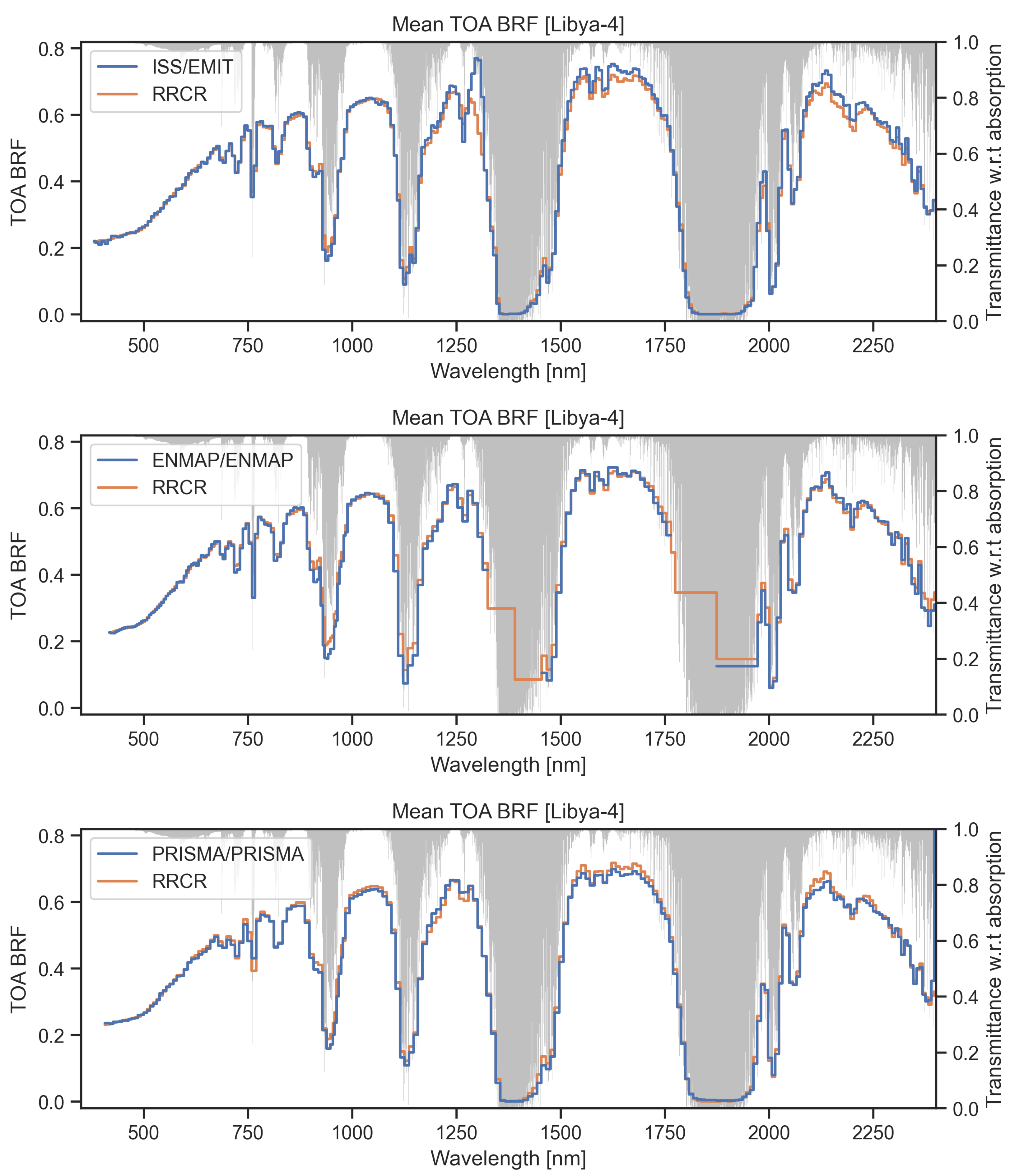
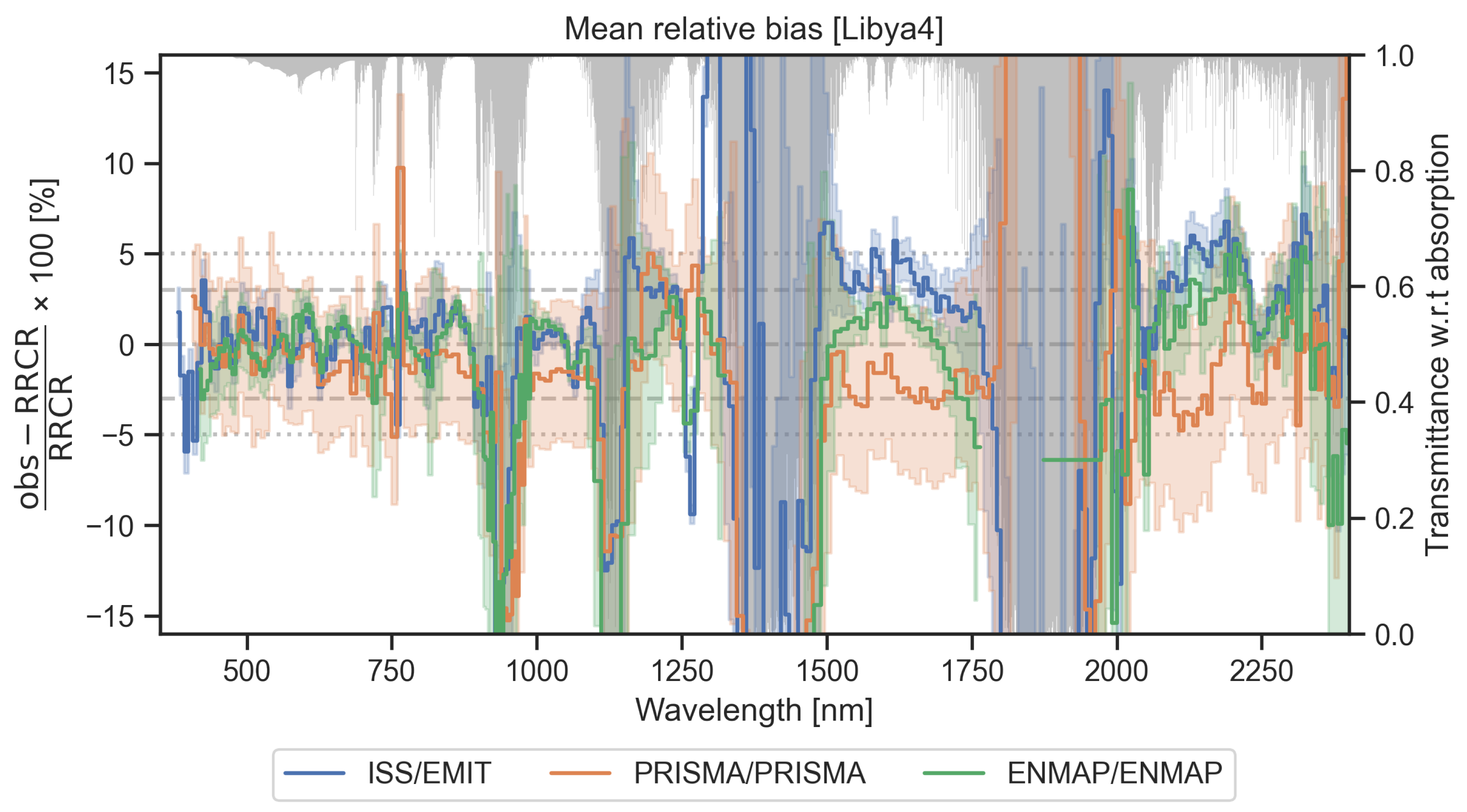
3.3.1. Libya4
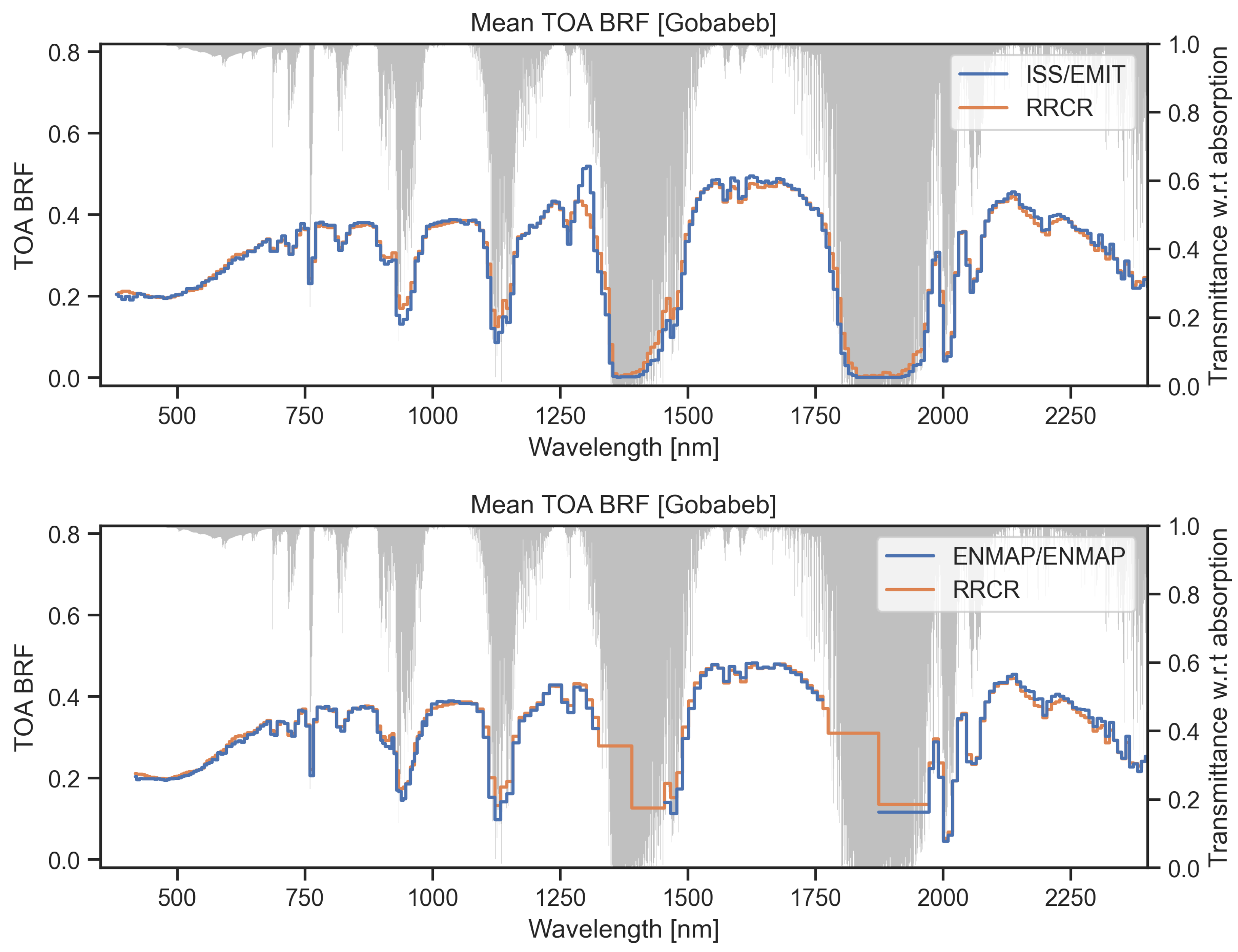
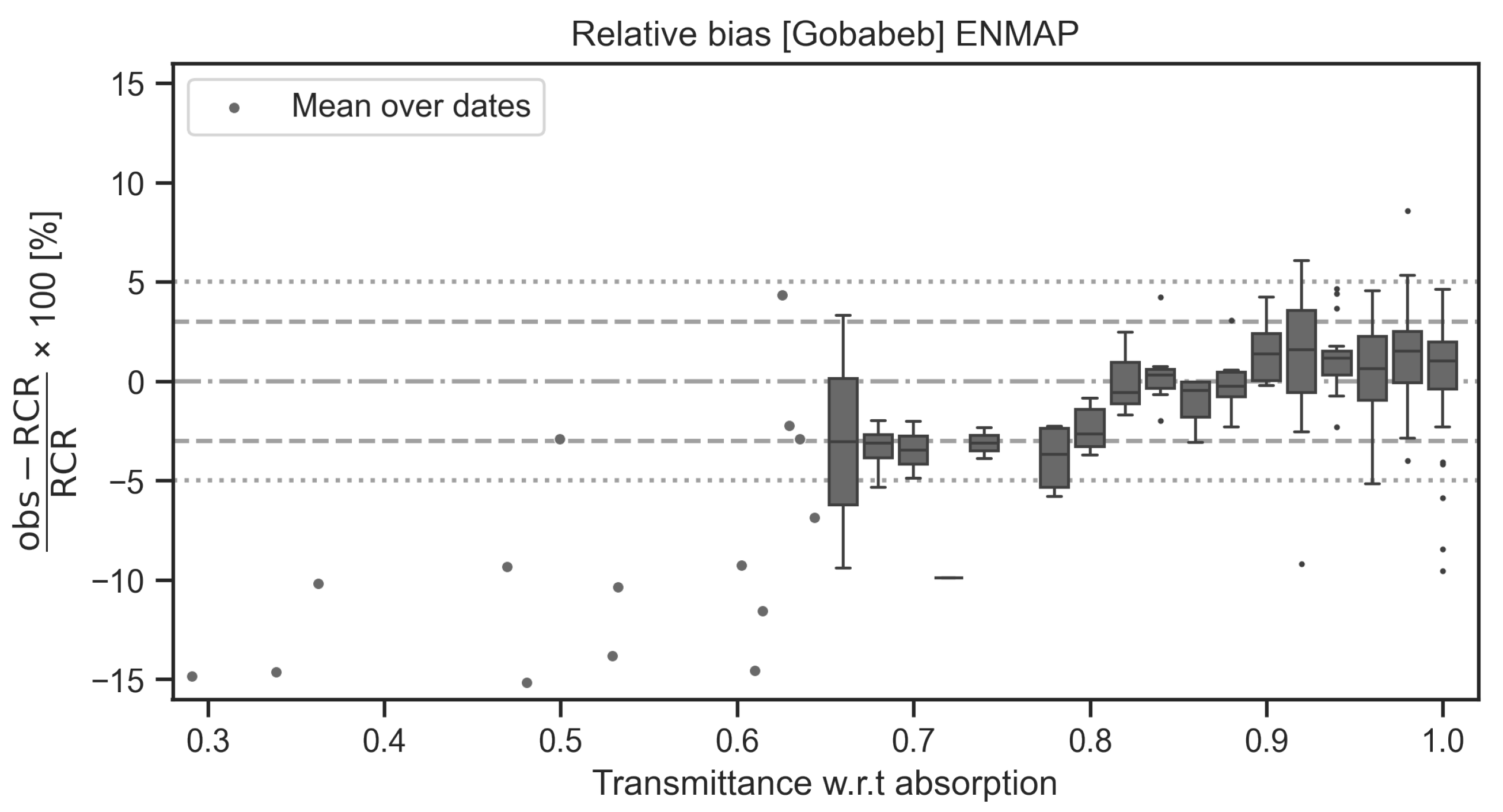
3.3.2. Gobabeb
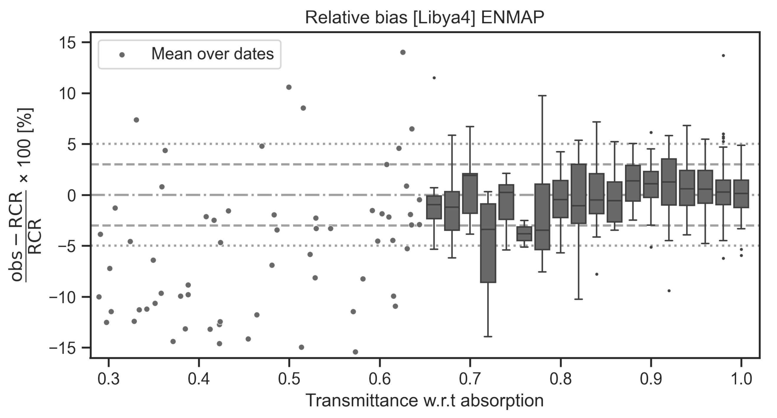
3.3.3. Evaluation of the Simulated RCR with Hyperspectral Observations
4. Discussion and Conclusions
Author Contributions
Funding
Institutional Review Board Statement
Informed Consent Statement
Data Availability Statement
Acknowledgments
Conflicts of Interest
References
- Boesch, H.; Brindley, H.; Carminati, F.; Fox, N.; Helder, D.; Hewison, T.; Houtz, D.; Hunt, S.; Kopp, G.; Mlynczak, M.; et al. SI-Traceable Space-Based Climate Observation System: A CEOS and GSICS Workshop. National Physical Laboratory, UK, 9–11 September 2019; Technical Report; National Physical Laboratory: Teddington, UK, 2019. [Google Scholar] [CrossRef]
- Cosnefroy, H.; Leroy, M.; Briottet, X. Selection and Characterization of Saharan and Arabian Desert Sites for the Calibration of Optical Satellite Sensors. Remote Sens. Environ. 1996, 58, 101–114. [Google Scholar] [CrossRef]
- Staylor, W.F. Degradation Rates of the AVHRR Visible Channel for the NOAA 6, 7, and 9 Spacecraft. J. Atmos. Ocean. Technol. 1990, 7, 411–423. [Google Scholar] [CrossRef]
- Bhatt, R.; Doelling, D.; Wu, A.; Xiong, X.; Scarino, B.; Haney, C.; Gopalan, A. Initial Stability Assessment of S-NPP VIIRS Reflective Solar Band Calibration Using Invariant Desert and Deep Convective Cloud Targets. Remote Sens. 2014, 6, 2809–2826. [Google Scholar] [CrossRef]
- Smith, D.L.; Mutlow, C.T.; Rao, C.R.N. Calibration Monitoring of the Visible and Near-Fnfrared Channels of Along-Track Scanning Radiometer-2 (ATSR-2) Using Stable Terrestrial Sites. Appl. Opt. 2002, 41, 515–523. [Google Scholar] [CrossRef]
- Wu, A.; Xiong, X.; Cao, C.; Angal, A. Monitoring MODIS Calibration Stability of Visible and Near-IR Bands from Observed Top-of-Atmosphere BRDF-normalized Reflectances over Libyan Desert and Antarctic Surfaces. In Proceedings of the Optical Engineering + Applications, San Diego, CA, USA, 10–14 August 2008; Volume 7081. [Google Scholar] [CrossRef]
- Govaerts, Y.; Clerici, M.; Clerbaux, N. Operational Calibration of the Meteosat Radiometer VIS Band. IEEE Trans. Geosci. Remote Sens. 2004, 42, 1900–1914. [Google Scholar] [CrossRef]
- Bacour, C.; Briottet, X.; Bréon, F.M.; Viallefont-Robinet, F.; Bouvet, M. Revisiting Pseudo Invariant Calibration Sites (PICS) Over Sand Deserts for Vicarious Calibration of Optical Imagers at 20 km and 100 km Scales. Remote Sens. 2019, 11, 1166. [Google Scholar] [CrossRef]
- Vermote, E.F.; Tanré, D.; Deuzé, J.L.; Herman, M.; Morcrette, J.J. Second Simulation of the Satellite Signal in the Solar Spectrum, 6S: An Overview. IEEE Trans. Geosci. Remote Sens. 1997, 35, 675–686. [Google Scholar] [CrossRef]
- Govaerts, Y.; Sterckx, S.; Adriaensen, S. Use of Simulated Reflectances over Bright Desert Target as an Absolute Calibration Reference. Remote Sens. Lett. 2013, 4, 523–531. [Google Scholar] [CrossRef]
- Giles, D.M.; Sinyuk, A.; Sorokin, M.G.; Schafer, J.S.; Smirnov, A.; Slutsker, I.; Eck, T.F.; Holben, B.N.; Lewis, J.R.; Campbell, J.R.; et al. Advancements in the Aerosol Robotic Network (AERONET) Version 3 Database—Automated near-Real-Time Quality Control Algorithm with Improved Cloud Screening for Sun Photometer Aerosol Optical Depth (AOD) Measurements. Atmos. Meas. Tech. 2019, 12, 169–209. [Google Scholar] [CrossRef]
- Kotchenova, S.Y.; Vermote, E.F.; Matarrese, R.; Klemm, F.J. Validation of a Vector Version of the 6S Radiative Transfer Code for Atmospheric Correction of Satellite Data. Part I: Path Radiance. Appl. Opt. 2006, 45, 6762–6774. [Google Scholar] [CrossRef] [PubMed]
- Govaerts, M.Y. Estimating the Accuracy of 1D Radiative Transfer Models over the Libya-4 Site. Technical Report RTMPV-WO1-2.3, Rayference. 2019. Available online: https://www.eradiate.eu/resources/docs/reports/report-assessment_calibration_libya4-2.3-20191007.pdf (accessed on 20 March 2025).
- Govaerts, Y.; Nollet, Y.; Leroy, V. Radiative Transfer Model Comparison with Satellite Observations over CEOS Calibration Site Libya-4. Atmosphere 2022, 13, 1759. [Google Scholar] [CrossRef]
- Leroy, V.; Nollet, Y.; Schunke, S.; Misk, N.; Marton, N.; Govaerts, Y. Eradiate Radiative Transfer Model. Version 0.29.2. 2024. Available online: https://github.com/eradiate/eradiate (accessed on 25 March 2025).
- Ruddick, K.G.; Bialek, A.; Brando, V.E.; De Vis, P.; Dogliotti, A.I.; Doxaran, D.; Goryl, P.; Goyens, C.; Kuusk, J.; Spengler, D.; et al. HYPERNETS: A network of automated hyperspectral radiometers to validate water and land surface reflectance (380–1680 nm) from all satellite missions. Front. Remote Sens. 2024, 5, 1372085. [Google Scholar] [CrossRef]
- Bialek, A.; Greenwell, C.; Lamare, M.; Meygret, A.; Marcq, S.; Lacherade, S.; Woolliams, E.; Berthelot, B.; Bouvet, M.; King, M.; et al. New radiometric calibration site located at Gobabeb, Namib desert. In Proceedings of the 2016 36th IEEE International Geoscience and Remote Sensing Symposium, IGARSS, Beijing, China, 10–15 July 2016; pp. 6094–6097. [Google Scholar] [CrossRef]
- European Space Agency; EU. Copernicus DEM—Global and European Digital Elevation Model. 2022. Available online: https://dataspace.copernicus.eu/explore-data/data-collections/copernicus-contributing-missions/collections-description/COP-DEM (accessed on 20 March 2025). [CrossRef]
- Govaerts, Y.M. Sand Dune Ridge Alignment Effects on Surface BRF over the Libya-4 CEOS Calibration Site. Sensors 2015, 15, 3453–3470. [Google Scholar] [CrossRef]
- Rahman, H.; Pinty, B.; Verstraete, M.M. Coupled Surface-Atmosphere Reflectance (CSAR) Model. 2. Semiempirical Surface Model Usable with NOAA Advanced Very High Resolution Radiometer Data. J. Geophys. Res. 1993, 98, 20791–20801. [Google Scholar] [CrossRef]
- Luffarelli, M.; Govaerts, Y. Joint Retrieval of Surface Reflectance and Aerosol Properties with Continuous Variation of the State Variables in the Solution Space—Part 2: Application to Geostationary and Polar-Orbiting Satellite Observations. Atmos. Meas. Tech. 2019, 12, 791–809. [Google Scholar] [CrossRef]
- Hersbach, H.; Bell, B.; Berrisford, P.; Biavati, G.; Horányi, A.; Muñoz Sabater, J.; Nicolas, J.; Peubey, C.; Radu, R.; Rozum, I.; et al. ERA5 Hourly Data on Single Levels from 1940 to Present. 2023. Available online: https://cds.climate.copernicus.eu/datasets/reanalysis-era5-single-levels?tab=overview (accessed on 20 March 2025). [CrossRef]
- Kinne, S. Aerosol Radiative Effects with MACv2. Atmos. Chem. Phys. 2019, 19, 10919–10959. [Google Scholar] [CrossRef]
- Nicodemus, F.E.; Richmond, J.C.; Hsia, J.J.; Ginsberg, I.W.; Limperis, T. Geometrical Considerations and Nomenclature for Reflectance; Technical Report NBS MONO 160; National Bureau of Standards: Gaithersburg, MD, USA; Washington, DC, USA, 1977. [Google Scholar] [CrossRef]
- GUM. Evaluation of Measurement Data—An Introduction to the “Guide to the Expression of the Uncertainty in Measurement” and Related Documents. GUM JCGM 104:2009, BIPM, Paris. 2009. Available online: https://www.bipm.org/documents/20126/2071204/JCGM_104_2009.pdf/19e0a96c-6cf3-a056-4634-4465c576e513?version=1.8&download=true (accessed on 17 March 2025).
- NPL. comet_maths toolkit. 2023. Available online: https://www.comet-toolkit.org/tools/comet_maths/ (accessed on 2 March 2025).
- Dupiau, A.; Jacquemoud, S.; Briottet, X.; Fabre, S.; Viallefont-Robinet, F.; Philpot, W.; Di Biagio, C.; Hébert, M.; Formenti, P. MARMIT-2: An improved version of the MARMIT model to predict soil reflectance as a function of surface water content in the solar domain. Remote Sens. Environ. 2022, 272, 112951. [Google Scholar] [CrossRef]
- Lavergne, T.; Kaminski, T.; Pinty, B.; Taberner, M.; Gobron, N.; Verstraete, M.; Voßbeck, M.; Widlowski, J.L.; Giering, R. An RPV Model Inversion Package Using Adjoint and Hessian Codes. In Proceedings of the International Meeting on Data Assimilation in Carbon Cycle Science, Edinburgh, UK, 9–11 May 2006. [Google Scholar]
- Benedetti, A.; Morcrette, J.J.; Boucher, O.; Dethof, A.; Engelen, R.J.; Fisher, M.; Flentje, H.; Huneeus, N.; Jones, L.; Kaiser, J.W.; et al. Aerosol Analysis and Forecast in the European Centre for Medium-Range Weather Forecasts Integrated Forecast System: 2. Data Assimilation. J. Geophys. Res. Atmos. 2009, 114, 2008JD011115. [Google Scholar] [CrossRef]
- Gueymard, C.A.; Yang, D. Worldwide Validation of CAMS and MERRA-2 Reanalysis Aerosol Optical Depth Products Using 15 Years of AERONET Observations. Atmos. Environ. 2020, 225, 117216. [Google Scholar] [CrossRef]
- Inness, A.; Ades, M.; Agustí-Panareda, A.; Barré, J.; Benedictow, A.; Blechschmidt, A.M.; Dominguez, J.J.; Engelen, R.; Eskes, H.; Flemming, J.; et al. The CAMS Reanalysis of Atmospheric Composition. Atmos. Chem. Phys. 2019, 19, 3515–3556. [Google Scholar] [CrossRef]
- Agustí-Panareda, A.; Barré, J.; Massart, S.; Inness, A.; Aben, I.; Ades, M.; Baier, B.C.; Balsamo, G.; Borsdorff, T.; Bousserez, N.; et al. Technical Note: The CAMS Greenhouse Gas Reanalysis from 2003 to 2020. Atmos. Chem. Phys. 2023, 23, 3829–3859. [Google Scholar] [CrossRef]
- Leroy, V.; Schunke, S.; Franceschini, L.; Misk, N.; Govaerts, Y. Impact of atmospheric vertical profile on hyperspectral simulations over bright desert pseudo-invariant calibration site. Eur. J. Remote Sens. 2024, 57, 2389798. [Google Scholar] [CrossRef]
- Dubovik, O.; Sinyuk, A.; Lapyonok, T.; Holben, B.N.; Mishchenko, M.; Yang, P.; Eck, T.F.; Volten, H.; Munoz, O.; Veihelmann, B.; et al. Application of Spheroid Models to Account for Aerosol Particle Nonsphericity in Remote Sensing of Desert Dust. J. Geophys.-Res.-Atmos. 2006, 111, 11208. [Google Scholar] [CrossRef]
- Dubovik, O.; Fuertes, D.; Litvinov, P.; Lopatin, A.; Lapyonok, T.; Doubovik, I.; Xu, F.; Ducos, F.; Chen, C.; Torres, B.; et al. A Comprehensive Description of Multi-Term LSM for Applying Multiple a Priori Constraints in Problems of Atmospheric Remote Sensing: GRASP Algorithm, Concept, and Applications. Front. Remote Sens. 2021, 2, 706851. [Google Scholar] [CrossRef]
- Ali, M.A.; Nichol, J.E.; Bilal, M.; Qiu, Z.; Mazhar, U.; Wahiduzzaman, M.; Almazroui, M.; Islam, M.N. Classification of aerosols over Saudi Arabia from 2004–2016. Atmos. Environ. 2020, 241, 117785. [Google Scholar] [CrossRef]
- Hemeret, F.; Formenti, P.; Di-Biagio, C.; Language, B.; Chevaillier, S.; Féron, A.; Cazaunau, M.; Torres-Sánchez, R.; Piketh, S.; Engelbrecht, F.; et al. New observations of climate-relevant properties of atmospheric aerosols in Namibia, southern Africa. Technical Report EGU23-465, Copernicus Meetings. In Proceedings of the EGU23, Vienna, Austria, 23–28 April 2023. [Google Scholar] [CrossRef]
- EUROCHAMP. EUROCHAMP Data Centre. 2023. Available online: https://data.eurochamp.org (accessed on 2 January 2025).
- Hess, M.; Koepke, P.; Schult, I. Optical Properties of Aerosols and Clouds: The Software Package OPAC. Bull. Am. Meteorol. Soc. 1998, 79, 831–844. [Google Scholar] [CrossRef]
- S2 MSI ESL team. Sentinel-2 Annual Performance Report—Year 2023. Technical Report OMPC.CS.APR.003, ESA. 2024. Available online: https://sentiwiki.copernicus.eu/__attachments/1673423/OMPC.CS.APR.003%20-%20S2%20MSI%20Annual%20Performance%20Report%202023%20-%201.0.pdf?inst-v=42dc07dd-44ef-491c-a236-c4c0594343a7 (accessed on 20 March 2025).
- Misk, N.; Nollet, Y.; Franceschini, L.; Govaerts, Y. Analysis of the Impact of Water Vapour on Sentinel-2 MSI Bands 8 and 8a TOA Reflectance. Available online: https://eradiate.eu/resources/docs/reports/report-analysis_water_s2_8_8a-1.0-20220902.pdf (accessed on 18 March 2025).
- Coddington, O.M.; Richard, E.C.; Harber, D.; Pilewskie, P.; Woods, T.N.; Chance, K.; Liu, X.; Sun, K. The TSIS-1 Hybrid Solar Reference Spectrum. Geophys. Res. Lett. 2021, 48, e2020GL091709. [Google Scholar] [CrossRef]
- Xiong, X.; Barnes, W. An overview of MODIS radiometric calibration and characterization. Adv. Atmos. Sci. 2006, 23, 69–79. [Google Scholar] [CrossRef]
- Lamquin, N.; Clerc, S.; Bourg, L.; Donlon, C. OLCI A/B Tandem Phase Analysis, Part 1: Level 1 Homogenisation and harmonization. Remote Sens. 2020, 12, 1804. [Google Scholar] [CrossRef]
- Fougnie, B. Improvement of the PARASOL Radiometric In-Flight Calibration Based on Synergy Between Various Methods Using Natural Targets. IEEE Trans. Geosci. Remote Sens. 2016, 54, 2140–2152. [Google Scholar] [CrossRef]
- Anderson, G.P.; Clough, S.A.; Kneizys, F.X.; Chetwynd, J.H.; Shettle, E.P. AFGL Atmospheric Constituent Profiles (0.120 km). 1986. Available online: https://ui.adsabs.harvard.edu/abs/1986afgl.rept.....A/abstract (accessed on 12 May 2025).
- De Vis, P.; Howes, A.; Vanhellemont, Q.; Bialek, A.; Morris, H.; Sinclair, M.; Ruddick, K. Feasibility of satellite vicarious calibration using HYPERNETS surface reflectances from Gobabeb and Princess Elisabeth Antarctica sites. Front. Remote Sens. 2024, 5, 1323998. [Google Scholar] [CrossRef]
- Formenti, P. A New Station for Long-Term In Situ Observations of Optical and Microphysical Properties of Aerosols in Gobabeb, Namibia. 2023. Available online: https://earth.esa.int/documents/20142/4300037/10-QA4EO_CalVal_WS4_Formenti.pdf (accessed on 25 March 2025).
- ASI. PRISMA Algorithm Theoretical Basis Document. 2021. Available online: https://prisma.asi.it/missionselect/docs/PRISMA%20ATBD_v1.pdf (accessed on 20 March 2025).
- Storch, T.; Honold, H.P.; Chabrillat, S.; Habermeyer, M.; Tucker, P.; Brell, M.; Ohndorf, A.; Wirth, K.; Betz, M.; Kuchler, M.; et al. The EnMAP imaging spectroscopy mission towards operations. Remote Sens. Environ. 2023, 294, 113632. [Google Scholar] [CrossRef]
- Coleman, R.W.; Thompson, D.R.; Brodrick, P.G.; Ben-Dor, E.; Cox, E.; García-Pando, C.P.; Hoefen, T.; Kokaly, R.; Meyer, J.M.; Ochoa, F.; et al. An Accuracy Assessment of the Surface Reflectance Product from the EMIT Imaging Spectrometer. 2024. Available online: https://essopenarchive.org/users/751176/articles/722321-an-accuracy-assessment-of-the-surface-reflectance-product-from-the-emit-imaging-spectrometer?commit=676d1a5d345289a86c1384f61035e235f2616f33 (accessed on 23 March 2025). [CrossRef]
- Thompson, D.R.; Green, R.O.; Bradley, C.; Brodrick, P.G.; Mahowald, N.; Dor, E.B.; Bennett, M.; Bernas, M.; Carmon, N.; Chadwick, K.D.; et al. On-orbit calibration and performance of the EMIT imaging spectrometer. Remote Sens. Environ. 2024, 303, 113986. [Google Scholar] [CrossRef]


| Name | Lon. | Lat. | Elevation | Size |
|---|---|---|---|---|
| Libya-4 | 23.42 | 28.67 | 130 (11) | 20 |
| Gobabeb | 15.12 | −23.60 | 498 (7) | 2 |
| Platform | Radiom. | Data Source | Product | Spectral Bands | Years | N-Libya4 | N-Gobabeb |
|---|---|---|---|---|---|---|---|
| AQUA/TERRA | MODIS | NASA EarthData LAADS/LP DAAC | MOD021KM MYD021KM MOD35_L2 MYD35_L2 | B01–B10 | 2005, 2006 | 270/240 | 269/267 |
| S2A | MSI | ESA Copernicus Data Space Ecosystem | S2A_MSIL1C | B1–B7, B8A, B11, B12 | 2018 | 31 | 31 |
| S3A/B | OLCI | ESA Copernicus Data Space Ecosystem | S3A_OL_1_EFR S3B_OL_1_EFR | Oa01–Oa11, Oa16–Oa18, Oa21 | 2021–2022 | 148 | 204 |
| MSG-4 | SEVIRI | EUMETSAT Data Store | MSG15, HRSEVIRI | VIS06, NIR16 | 2020 | 5542 | 0 |
| PARASOL | POLDER | AERIS/ICARE Data and Services Center | POLDER3_L1B-BG1 | 0443, 0490, 0565, 0670, 0865, 1020 | 2008–2009 | 3405 | 0 |
| Instrument | Data Source | Product | Years | N-Libya4 | N-Gobabeb |
|---|---|---|---|---|---|
| EMIT | NASA | EMIT_L1B_RAD | 2022, | 6 | 3 |
| EarthData | EMIT_L1B_OBS | 2023 | |||
| LAADS | EMIT_L2A_MASK | ||||
| DAAC | EMIT_L2A_RFL | ||||
| EMIT_L2A_RFLUNCERT | |||||
| PRISMA | ASI Prisma | PRS_L1_STD | 2019, | 28 | 0 |
| catalogue | 2020, | ||||
| client | 2021, | ||||
| 2022, | |||||
| 2023, | |||||
| ENMAP | DLR EOC | ENMAP.HSI.L1C | 2022, | 34 | 26 |
| EOWEB | 2023 | ||||
| GeoPortal |
Disclaimer/Publisher’s Note: The statements, opinions and data contained in all publications are solely those of the individual author(s) and contributor(s) and not of MDPI and/or the editor(s). MDPI and/or the editor(s) disclaim responsibility for any injury to people or property resulting from any ideas, methods, instructions or products referred to in the content. |
© 2025 by the authors. Licensee MDPI, Basel, Switzerland. This article is an open access article distributed under the terms and conditions of the Creative Commons Attribution (CC BY) license (https://creativecommons.org/licenses/by/4.0/).
Share and Cite
Luffarelli, M.; Misk, N.; Leroy, V.; Govaerts, Y. Elaboration of Simulated Hyperspectral Calibration Reference over Pseudo-Invariant Calibration Reference. Atmosphere 2025, 16, 583. https://doi.org/10.3390/atmos16050583
Luffarelli M, Misk N, Leroy V, Govaerts Y. Elaboration of Simulated Hyperspectral Calibration Reference over Pseudo-Invariant Calibration Reference. Atmosphere. 2025; 16(5):583. https://doi.org/10.3390/atmos16050583
Chicago/Turabian StyleLuffarelli, Marta, Nicolas Misk, Vincent Leroy, and Yves Govaerts. 2025. "Elaboration of Simulated Hyperspectral Calibration Reference over Pseudo-Invariant Calibration Reference" Atmosphere 16, no. 5: 583. https://doi.org/10.3390/atmos16050583
APA StyleLuffarelli, M., Misk, N., Leroy, V., & Govaerts, Y. (2025). Elaboration of Simulated Hyperspectral Calibration Reference over Pseudo-Invariant Calibration Reference. Atmosphere, 16(5), 583. https://doi.org/10.3390/atmos16050583