Estimation of Biomass Burning Emissions in South and Southeast Asia Based on FY-4A Satellite Observations

Abstract

In recent years, frequent open biomass burning (OBB) activities such as agricultural residue burning and forest fires have led to severe air pollution and carbon emissions across South and Southeast Asia (SSEA). We selected this area as our study area and divided it into two sub-regions based on climate characteristics and geographical location: the South Asian Subcontinent (SEAS), which includes India, Laos, Thailand, Cambodia, etc., and Equatorial Asia (EQAS), which includes Indonesia, Malaysia, etc. However, existing methods—primarily emission inventories relying on burned area, fuel load, and emission factors—often lack accuracy and temporal resolution for capturing fire dynamics. Therefore, in this study, we employed high-resolution fire point data from China’s Feng Yun-4A (FY-4A) geostationary satellite and the Fire Radiative Power (FRP) method to construct a daily OBB emission inventory at a 5 km resolution in this region for 2020–2022. The results show that the average annual emissions of carbon (C), carbon dioxide (CO₂), carbon monoxide (CO), methane (CH₄), non-methane organic gases (NMOGs), hydrogen (H₂), nitrogen oxide (NO_X), sulfur dioxide (SO₂), fine particulate matter (PM_2.5), total particulate matter (TPM), total particulate carbon (TPC), organic carbon (OC), black carbon (BC), ammonia (NH₃), nitric oxide (NO), nitrogen dioxide (NO₂), non-methane hydrocarbons (NMHCs), and particulate matter ≤ 10 μm (PM₁₀) are 178.39, 598.10, 33.11, 1.44, 4.77, 0.81, 1.02, 0.28, 3.47, 5.58, 2.29, 2.34, 0.24, 0.58, 0.43, 0.99, 1.87, and 3.84 Tg/a, respectively. Taking C emission as an example, 90% of SSEA’s emissions come from SEAS, especially concentrated in Laos and western Thailand. Due to the La Niña climate anomaly in 2021, emissions surged, while EQAS showed continuous annual growth at 16.7%. Forest and woodland fires were the dominant sources, accounting for over 85% of total emissions. Compared with datasets such as the Global Fire Emissions Database (GFED) and the Global Fire Assimilation System (GFAS), FY-4A showed stronger sensitivity and regional adaptability, especially in SEAS. This work provides a robust dataset for carbon source identification, air quality modeling, and regional pollution control strategies.

1. Introduction

In recent years, fires caused by natural or human causes have become a major public concern, such as the wildfires in South Korea and the wildfires in California [1,2]. According to the Global Fire Emissions Database 5 (GFED5), the average annual global carbon dioxide (CO₂) emissions from biomass burning fires between 2002 and 2022 were 11.28 Gt CO₂ yr⁻¹, with CO₂ emissions reaching 9.89 Gt in 2022 [3]. The increasing frequency of fires has led to severe air pollution, which has profound impacts on climate change and human health, particularly in developing countries, especially in South and Southeast Asia (SSEA), where the effects are intensifying [4,5,6]. The large-scale open biomass burning (OBB) throughout the year has resulted in concentrations of trace gases, including carbon monoxide (CO), nitrogen oxide (NO_x), non-methane volatile organic compounds (NMVOCs), sulfur dioxide (SO₂), and ammonia (NH₃), as well as fine particulate matter (PM_2.5), frequently exceeding World Health Organization (WHO) standards [7]. These burning activities release substantial carbon emissions, which not only negatively impact the global climate system but also pose significant health risks to local populations. Deforestation, accidental fires, firewood burning, agricultural residue burning, and peatland burning have become major OBB fire types globally [8]. Establishing an OBB emission inventory has become an urgent task to quantify the contribution of local biomass burning to regional and global carbon emissions, providing a scientific basis for the development of mitigation policies and strategies.

Previous studies have explored various methods for estimating biomass burning emissions [9,10,11]. The emission inventory approach, proposed by the Intergovernmental Panel on Climate Change (IPCC), is a method for estimating greenhouse gas emissions. According to the inventory list, a function is established for each fire type relating activity data to emission factors to estimate the emissions [12]. When calculating OBB emissions, estimations can be made based on the burned area (km²), available biomass (kg·m⁻²), combustion efficiency (%), and emission factors for various pollutants (g·kg⁻¹) [13,14]. The GFED5 quantifies trace gas and aerosol emissions from global biomass burning by utilizing satellite-derived burn area data, fuel load simulated by biogeochemical models, humidity-adjusted combustion factors, and land cover-based emission factors [3]. This dataset provides monthly global OBB emission data at a resolution of 0.25° × 0.25° (g/m²/month) for different vegetation fires from 1997 to now [3]. However, van der Werf et al. (2017) pointed out that due to uncertainties in the parameters involved, GFED simulation results deviate by approximately 14% from the field observations of available biomass fuels [12].

Additionally, the National Center for Atmospheric Research (NCAR) has developed a fire emission inventory using the FINN (Fire Inventory from NCAR v2.5) model, which estimates high-resolution global OBB emissions [15]. However, FINN results are mainly based on fire count data [16]. The actual burned area for each fire event can vary significantly, and using fire count data as a proxy for the affected area may lead to significant errors in emission estimates.

The Fire Radiative Power (FRP) method, which is based on real-time observations of fire points using platforms such as satellite remote sensing, obtains the radiative energy of fires and estimates biomass burning carbon emissions by multiplying the biological consumption with the biomass combustion conversion factor [17,18,19]. Research by Freeborn et al. (2008) indicated that biomass burning and FRP are not significantly influenced by surface vegetation cover types [20]. Therefore, the fuel mass consumed in OBB can be converted using a conversion rate constant, avoiding errors caused by inaccurate burn area inversions and fire count statistics. This method overcomes the challenges of traditional biomass burning emission estimation methods, which cannot monitor carbon emissions from small fire points [21]. The Global Fire Assimilation System (GFAS) data, based on the FRP method, provides daily emission inventory products with a resolution of 0.1° × 0.1° [22,23].

Currently, several OBB emission datasets have been developed globally, including the GFED, the GFAS, and the Fire Emissions and Energy Research (FEER). However, these methods are highly dependent on the accuracy of fire detection, especially the ability to identify small-scale fires, and the activity data used contain significant uncertainties, leading to limitations and unreliability in the estimation results [24]. Li et al. (2019) used FRP data from MODIS and the Geostationary Operational Environmental Satellite (GOES) to reconstruct the diurnal fire radiation cycle in the continental United States by fusing FRP data from polar-orbiting and geostationary satellites, demonstrating the effectiveness of geostationary satellites in estimating biomass burning emissions based on the FRP method [25]. In conclusion, most existing methods still rely on MODIS active fire products for research. Compared with MODIS, the Feng Yun-4A (FY-4A) satellite is located in geostationary orbit and offers higher temporal resolution, enabling continuous observation of the Earth’s surface at minute-level frequency and capturing fire point dynamics in real-time [26]. Additionally, its Advanced Geostationary Radiation Imager (AGRI) can acquire Earth cloud imagery in over 14 spectral bands with visible channels that reach a resolution of 0.5–1 km, making it capable of clearly identifying small fire points and their boundaries [26,27].

Global warming has led to an increase in the frequency of wildfires, with approximately 20 million fires occurring annually worldwide [28,29]. SSEA is among the most fire-prone regions globally, accounting for about 15% to 25% of global fire incidents [30]. Wildfires in this region contribute significantly to CO₂ emissions, with Southeast Asian peatlands, such as those in Indonesia’s Sumatra and Kalimantan [31]. Additionally, agricultural burning in the Ganges Plain of South India leads to severe air pollution every spring, causing significant haze [32,33]. Biomass burning also releases pollutants such as PM_2.5 and black carbon, which can cross borders and severely impact local development and public health [34,35]. Therefore, there is an urgent need to establish high-precision biomass burning emission inventories.

In this study, we used the Fire/Hot Spot Detection Product (FHS) from FY-4A AGRI to construct daily OBB emission inventories for South and Southeast Asia from 2020 to 2022 based on the FRP method, providing daily emissions of 18 pollutants, including carbon (C), CO₂, CO, methane (CH₄), non-methane organic gases (NMOGs), hydrogen (H₂), NO_x, SO₂, PM_2.5, total particulate matter (TPM), total particulate carbon (TPC), organic carbon (OC), black carbon (BC), NH₃, nitric oxide (NO), nitrogen dioxide (NO₂), non-methane hydrocarbons (NMHCs), and particulate matter ≤ 10 μm (PM₁₀). Furthermore, this study explores the spatial and temporal variation characteristics of emission inventory results across different regions and fire types in South and Southeast Asia (SSEA). This comprehensive, high-resolution OBB emission inventory serves as a valuable resource for air quality modeling, atmospheric transport simulations, and biogeochemical cycle studies. It provides a robust framework for understanding and analyzing the environmental impacts of OBB in SSEA.

2. Materials and Methods

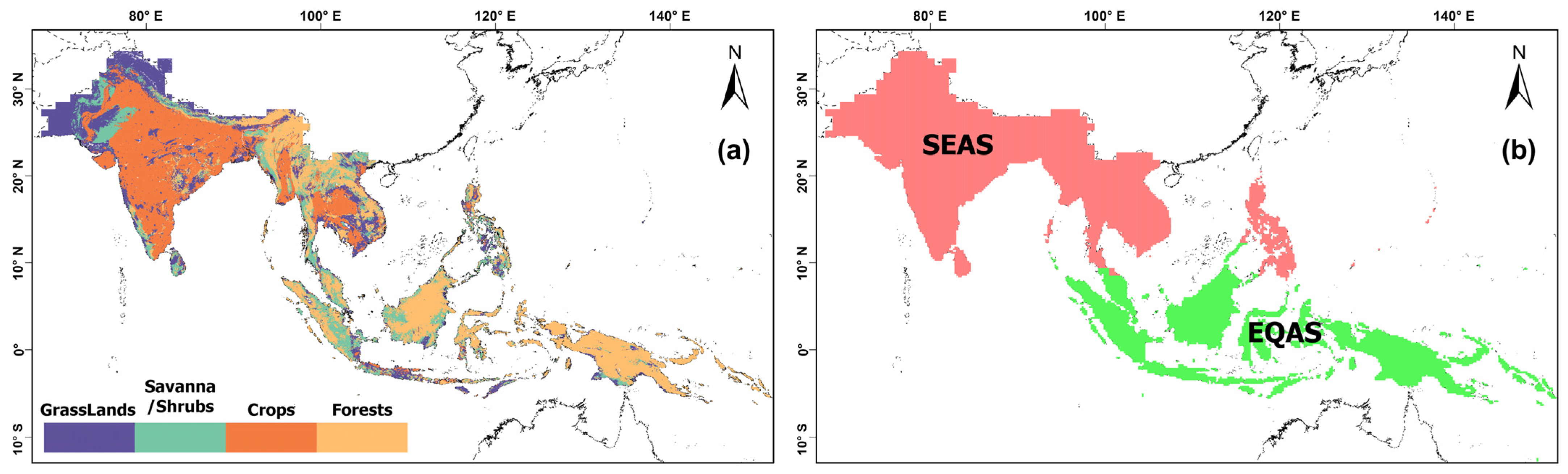
2.1. Study Area

SSEA is characterized by complex and diverse geographical environments (Figure 1a). Due to rapid population growth and limited land resources, large areas of forests have been degraded, exacerbating local climate change [36].

This study adopts the global biomass burning emission zoning framework proposed by van der Werf et al. (2006) and divides the study area (SSEA) into two standardized geographic units: Equatorial Asia (EQAS) and South Asia (SEAS) [37] (Figure 1b). This zoning scheme is based on the GFED, taking into account regional ecological types, providing a unified spatial reference for subsequent emission calculations and cross-regional comparative analysis [38].

2.2. Data

We innovatively employed the Fire/Hot spot detection product (FHS) of FY-4A as the active fire data. This product utilizes data from the FY-4A Advanced Geostationary Radiation Imager (AGRI), leveraging the sensitivity of mid-infrared channels to high-temperature heat sources and the spectral characteristics of clouds and vegetation across different AGRI channels to eliminate solar radiation interference [26]. It extracts fire spot information within the FY-4A observation range, estimates sub-pixel fire area and temperature, and generates fire distribution and intensity list products (2 km, 15 min interval) as well as thematic fire maps (http://satellite.nsmc.org.cn/DataPortal/cn/home/index.html, accessed on 3 April 2024) [39]. This product includes fire point pixel location, sub-pixel fire point area, fire point intensity, the administrative region and land use type of the fire point, and observation time. It provides continuous dynamic monitoring information for large-scale fire events and offers biomass burning fire information for the Asian region. To improve the detection accuracy of actual fire events, we aggregated spatially adjacent fire spots into 5 km × 5 km grid cells, as wildfires commonly consist of clustered ignition points. This approach allows each grid-based fire cluster to collectively represent the regional FRP and combustion intensity.

In this study, the MODIS Land Cover Climate Modeling Grid data (MCD12C1.061, https://lpdaac.usgs.gov/products/mcd12c1v061/, accessed on 13 November 2024) were used as the base land cover data [40]. Through spatial aggregation and reprojection, it provides global land cover information at a 0.05° resolution for the years 2001 to 2022. To avoid the parameter drift caused by heterogeneous vegetation in the International Geosphere–Biosphere Programme (IGBP) classification [41,42,43], the original 17 IGBP ecosystem classes were reclassified into four functional units (excluding water bodies and others): forest, woodland, cropland, and grassland (

Table 1. Reclassification of MOD12C1.061 in SSEA.

IGBP Description	Value	Reclassification Results
Evergreen Needleleaf Forests	1	forest
Evergreen Broadleaf Forests	2
Deciduous Needleleaf Forests	3
Deciduous Broadleaf Forests	4
Mixed Forests	5
Closed Shrublands	6	woodland
Open Shrublands	7
Woody Savannas	8
Savannas	9	grassland
Grasslands	10
Permanent Wetlands	11
Croplands	12	cropland
Urban and Built–up Lands	13	forest
Cropland/Natural Vegetation Mosaics	14	cropland
Permanent Snow and Ice	15	-
Barren	16	cropland
Water Bodies	0	-

).

2.3. Methods

This study estimates the OBB for the study area from 2020 to 2022 based on FRP. The core of the model lies in using FRP obtained from satellite remote sensing to infer biomass combustion emissions [44,45]. There is a strong linear relationship between the fire radiative energy (FRE, unit: MJ) and the dry matter mass ($M$, unit: kg) during biomass combustion, and this relationship is insensitive to vegetation type [44]. Therefore, the biomass emission ($E_i$, unit: g) can be calculated by first estimating the dry matter mass through the radiative energy and then multiplying by the corresponding emission factor (${EF}_i$, unit: g/kg), which reduces the uncertainty in the calculation results due to the large number of parameters involved. The calculation formula is as follows:

$$E_i=M\times {EF}_i$$

(1)

where $M$ represents the burned dry mass (kg), and ${EF}_i$ is the emission of specific substance $i$ in the fire grid unit, with values listed in

Table 2. Emission factors (g/kg) of different landcover.

	Cropland	Grassland	Forest	Woodland
C	449.00	494.60	480.00	489.42
CO2	1353.50 a	1686.00 b	1643.00 b	1681.00 b
CO	76.10 a	63.00 b	93.00 b	67.00 b
CH4	2.80 a	2.00 b	5.10 b	3.00 b
NMOG	9.80 a	28.20 b	51.90 b	24.80 b
H2	2.59 b	1.70 b	3.40 b	0.97 b
NOX	2.90 a	3.90 b	2.60 b	3.65 b
SO2	0.40 a	0.90 b	0.40 b	0.68 b
PM2.5	5.00 a	7.17 b	9.90 b	7.10 b
TPM	13.00 b	8.30 b	18.50 b	15.40 b
TPC	4.00 b	3.00 b	5.20 b	7.10 b
OC	2.00 b	2.60 b	4.70 b	3.70 b
BC	0.60 b	0.37 b	0.52 b	1.31 b
NH3	1.40 a	0.56 b	1.30 b	1.20 b
NO	1.18 b	2.16 b	0.90 b	0.77 b
NO2	2.99 b	3.22 b	3.60 b	2.58 b
NMHC	7.00 b	3.40 b	1.70 b	3.40 b
PM10	6.30 b	7.20 b	18.50 b	11.40 b

Data source description: ^a was from Yin et al. (2019) [46]. ^b was obtained from Akagi et al. (2011) [47], where the forest combustion factor specifically referred to the emission factor for tropical forests, as documented in their study. The combustion factors for C were determined by computing the mass fraction of carbon atoms in CO₂, CO, and CH₄.

.

$$M=FRE\times CR$$

(2)

$CR$ (unit: kg/MJ) is the conversion ratio used to convert $FRE$ to burned dry biomass (M). Roberts et al. (2005) found that $CR$ is 0.368 ± 0.015 kg/MJ [44], while Freeborn et al. (2008) reported a $CR$ of 0.453 ± 0.068 kg/MJ [20]. Therefore, in this study, we adopted the CR value of 0.368 kg/MJ for agricultural fires from Roberts et al. (2005) [44]. For other land use types, the $CR$ value was selected as the average value (0.411 kg/MJ) based on the method proposed by Lv et al. (2022) [45].

The FRE, which represents the total radiant energy of a grid cell within a day, is crucial for this study. Different from the MODIS satellite, the FY-4A is a geostationary satellite with a higher observation frequency. It can provide fire spot monitoring data with high temporal resolution, which is of great significance for tracking and simulating the changes of wildfires. For each set of fire spot data (with a resolution of 5 KM) after clustering, the FRP is first aggregated according to time points to obtain the total FRP value at each time point. Suppose the time series be $t_i\left(i=\mathrm{1,2},\dots ,n\right)$, and the corresponding FRP value be $FRP\left(t_i\right)$.

$$FRE={\int }_0^{24}FRP\left(t\right)dt$$

(3)

$FRP\left(t\right)$ is the fire radiative power at a certain moment $t$, and the total integral represents the total radiant energy of this grid within 24 h.

The biomass combustion is a dynamic process from the ignition to the extinction of the fire, and the FRP will gradually increase and then decrease [25]. Assuming the temporal variation of fire radiative power within a fire cluster follows a continuous function, we address the discontinuity in satellite observation cycles through interpolation and the simulation of fire growth and decay processes. This approach reconstructs the complete daily FRP curve, enabling the model to more accurately represent actual fire activity.

We propose that fires had already begun burning gradually prior to time $t_1$ (the first observation timestamp in the time series). To simulate this, the following enhanced model is employed:

$${FRP\left(t\right)}_{growth}={FRP}_{t_1}·e^{\beta \left(t-t_1\right)}$$

(4)

${FRP\left(t\right)}_{growth}$ represents the radiative power during the growth phase, ${FRP}_{t_1}$ denotes the initial radiative power at time $t_1$, $\beta$ is the growth coefficient ($\beta =0.5$), and $t_1$ is the ignition start time.

For the period after the final observation timestamp $t_n$, we simulate the fire’s gradual decay using the following attenuation model:

$${FRP\left(t\right)}_{decay}={FRP}_{t_n}·e^{-\gamma \left(t-t_n\right)}$$

(5)

${FRP\left(t\right)}_{decay}$ represents the radiative power during the decay phase, ${FRP}_{t_n}$ denotes the last observed radiative power at time $t_n$, $\gamma$ is the decay coefficient ($\gamma$ = 0.01), and $t_n$ marks the end of the observation period.

To estimate the total radiation energy (FRE) within a specific grid over the course of a day, the Piecewise Cubic Hermite Interpolating Polynomial (PCHIP) method was utilized to interpolate the limited data points within the same grid, extending them to finer time intervals. This interpolation also involved smoothing the radiation power data during the growth, observation, and decay phases, thereby generating a continuous radiation power curve. Finally, FRE was calculated using the trapezoidal rule for numerical integration (unit: MJ).

3. Results

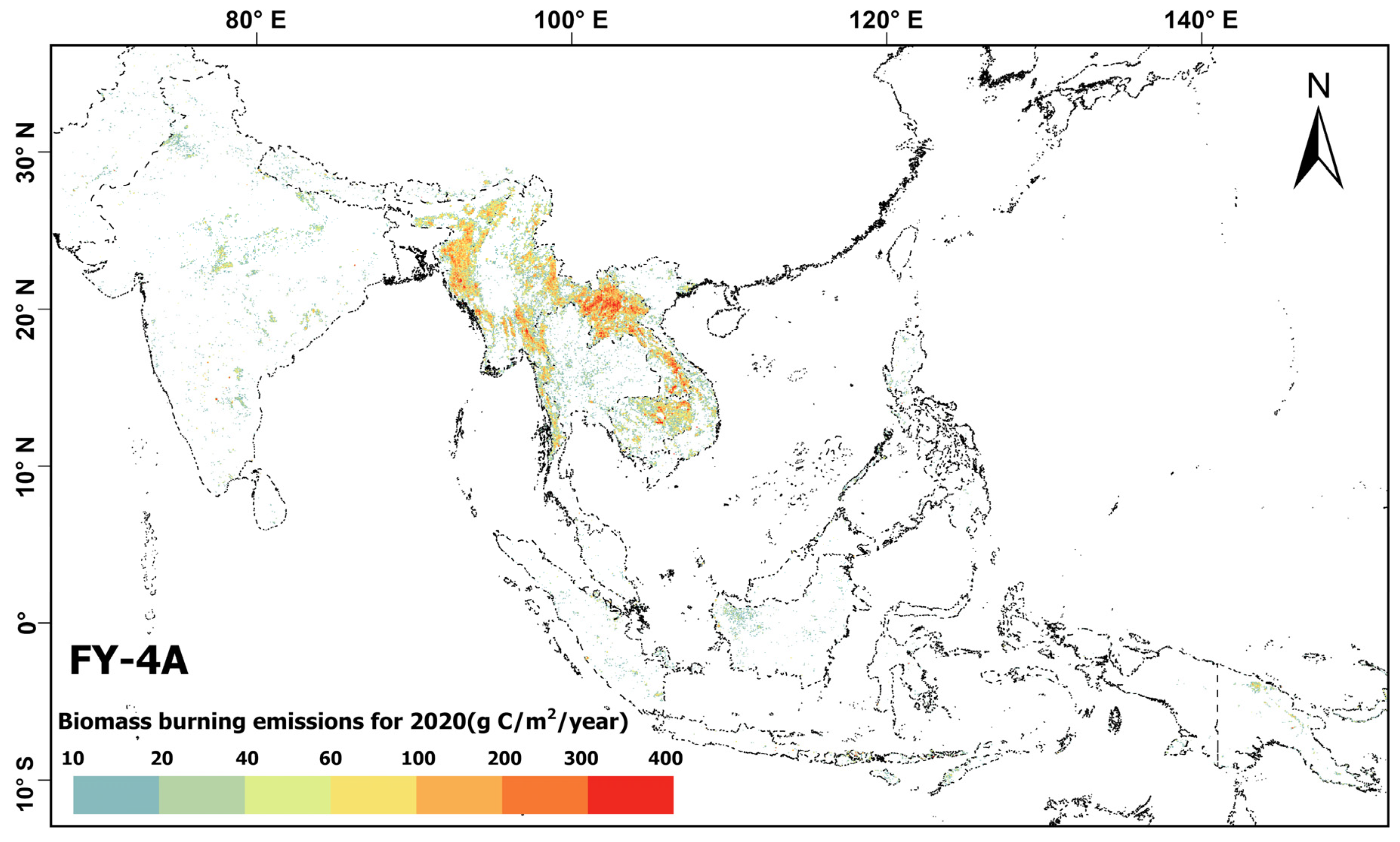
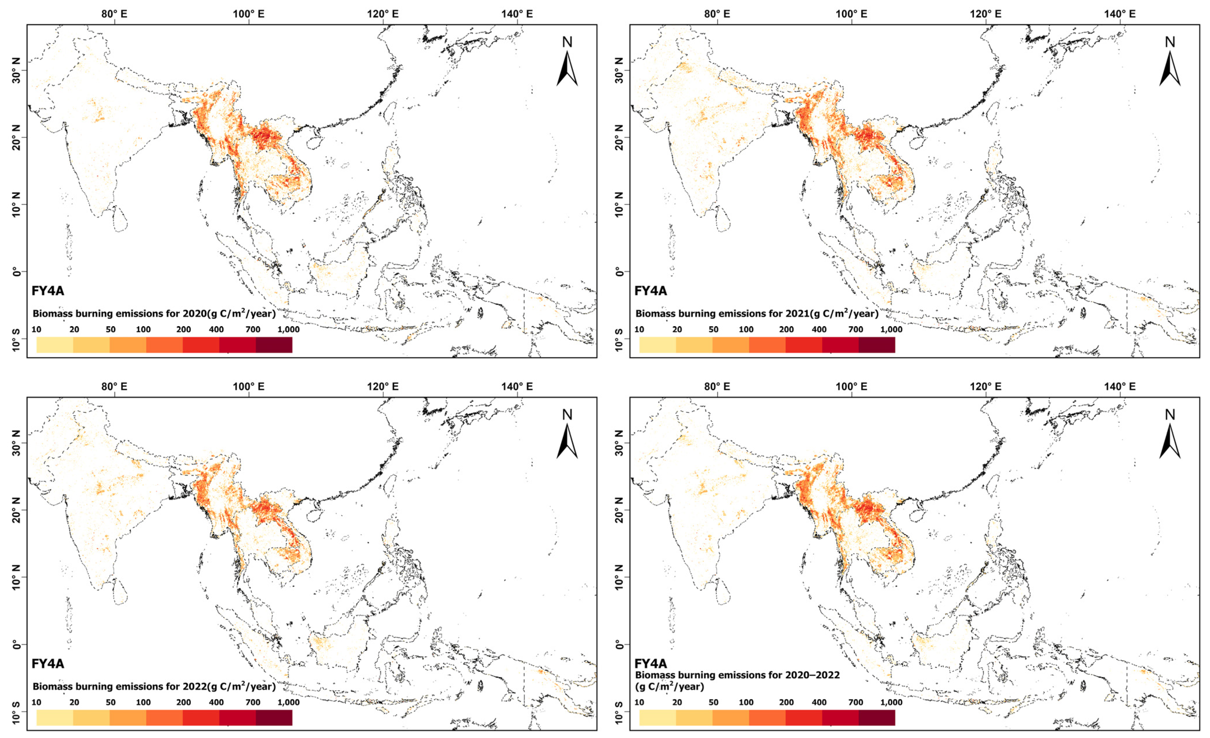
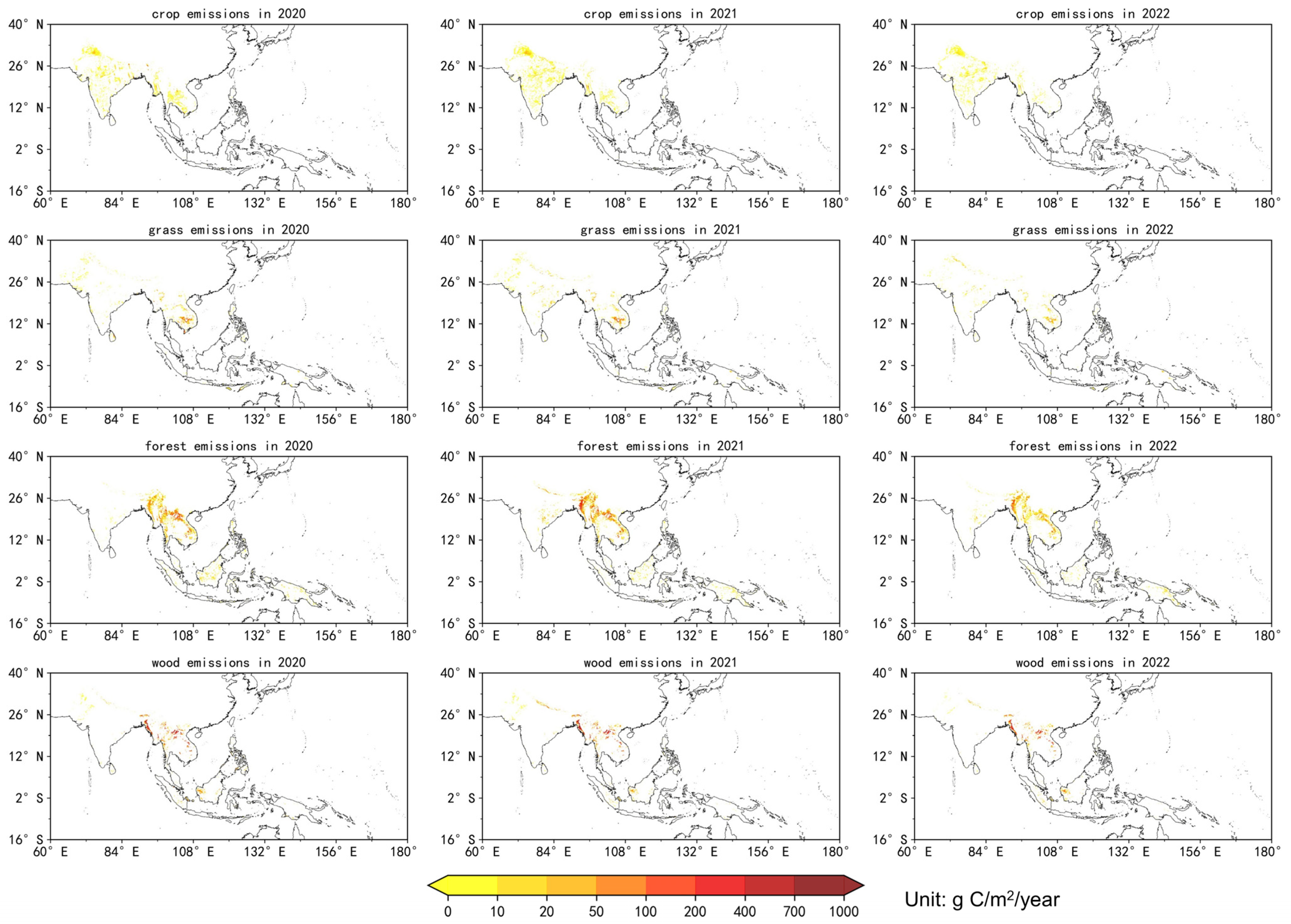
3.1. Spatial Patterns of OBB Emissions

In this section, we use net carbon (C) emissions as a representative measure to describe the characteristics of OBB emissions across the entire study area. Biomass burning emissions in SSEA exhibit distinct spatial distribution characteristics, with the annual average C emissions across the entire study area reaching 211.46 Tg from 2020 to 2022. Figure 2 illustrates the average C emissions in SSEA during this period. It is evident that the entire area of Laos, the western part of Thailand, the southern part of Cambodia, and the western region of Laos display significantly high emissions. In most parts of Laos, C emissions exceed 200 (g/C/m²/year). Additionally, the western and northeastern regions of Myanmar, as well as areas bordering Thailand, show notable C emissions. The central and northern parts of India also exhibit some C emissions, although to a lesser extent. In the EQAS region, no significant high values are observed. C emissions are primarily distributed as point sources in the northwest of Sumatra and Borneo in Indonesia, which shows good consistency with the distribution of local peatlands. Overall, the SEAS region accounts for 90% of the total C emissions in the entire study area.

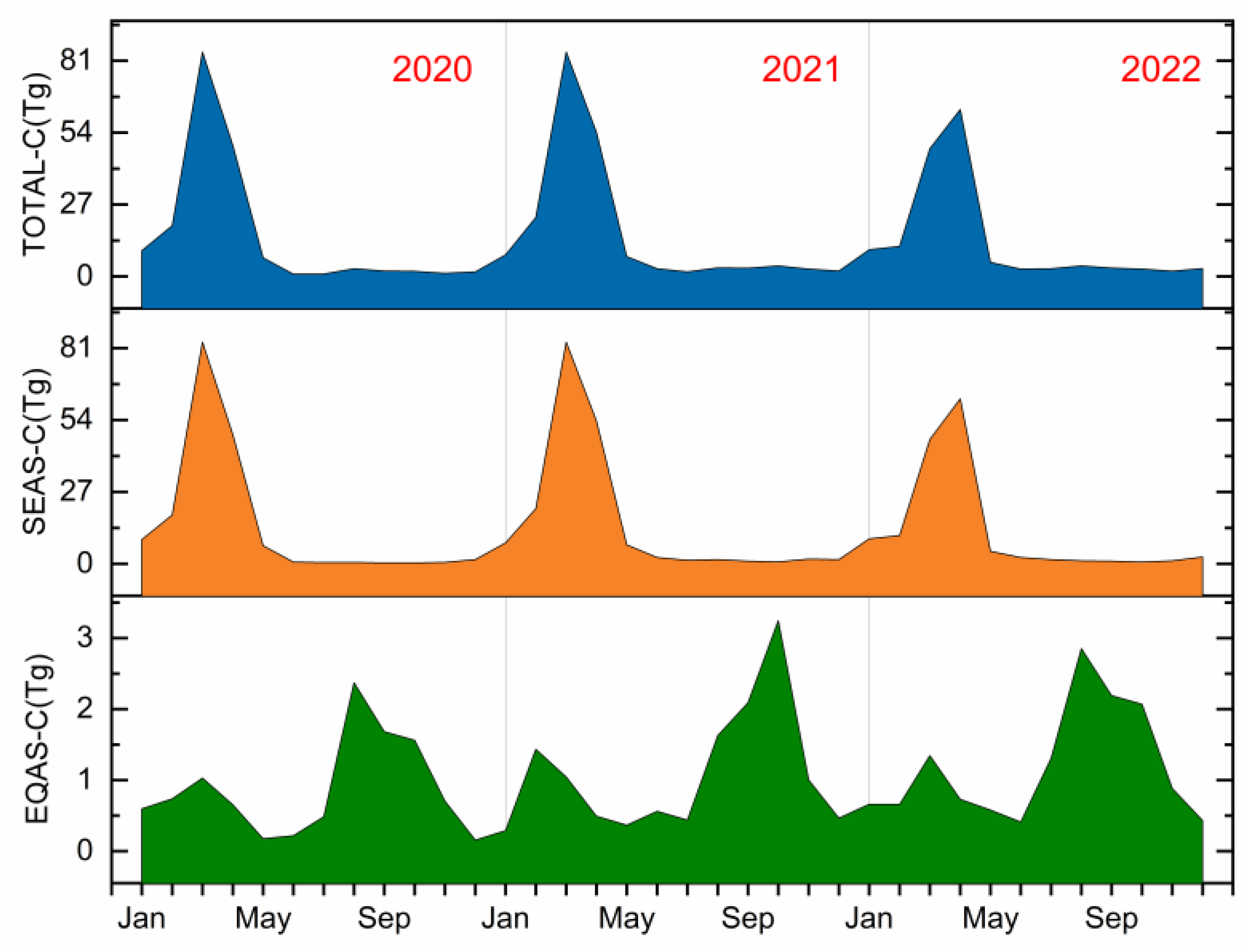
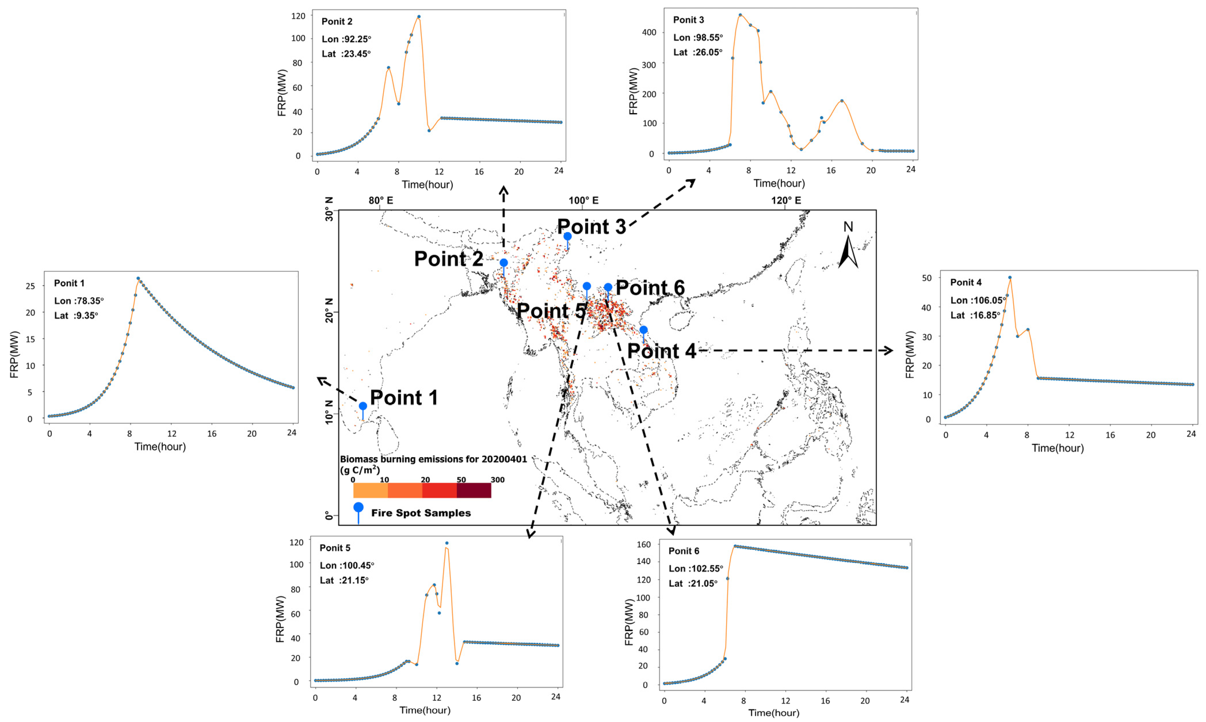
3.2. Temporal Patterns of OBB Emissions

We conducted a quantitative analysis of the spatiotemporal patterns of biomass burning carbon emissions in Southeast Asia from 2020 to 2022 (Figure 3). The results reveal substantial spatial heterogeneity and interannual variability across different countries. In India, fire occurrences in 2020 were primarily concentrated in the central region, with the annual OBB emissions reaching the lowest level within the study period. However, in the subsequent years (2021–2022), fire activity exhibited a notable spatial expansion toward the northern and southern regions, accompanied by a significant increase in OBB emissions. This interannual shift may be associated with changes in crop residue management practices driven by abnormal monsoon conditions. Notably, Laos consistently maintained high emission levels throughout the study period. The spatial hotspots were persistently located in the transitional zones between the Mekong River floodplains and the Annamite Mountains, suggesting a strong link to the long-standing practice of slash-and-burn agriculture in the region. In contrast, Cambodia experienced a marked decline in fire activity, particularly in the southern areas where carbon emissions substantially decreased. Fire occurrences in Thailand and Vietnam showed limited interannual fluctuations, with carbon emissions remaining relatively stable, indicating the sustained implementation of agricultural burning control policies in both countries.

In EQAS, peatland fires in Indonesia and Papua New Guinea emerged as a major concern. The increasing density of fire events in peatland areas contributed significantly to the rise in carbon emission shares, underscoring the heightened vulnerability of these ecosystems to fire-induced carbon release.

Additionally, we developed a high-resolution biomass burning emission inventory for the SSEA, quantitatively characterizing the spatiotemporal heterogeneity of 18 atmospheric pollutants during the period 2020–2022 (

Table 3. Annual OBB emissions inventory of 18 pollutants in the SEAS and EQAS regions from 2020 to 2022 (unit: Tg).

	SEAS			EQAS
	2020	2021	2022	2020	2021	2022
C	170.5822	183.0390	143.9476	10.3839	13.0756	14.1371
CO2	572.4475	613.6722	482.5472	34.6968	43.6592	47.2636
CO	31.3695	33.9839	26.7615	1.9934	2.5279	2.6993
CH4	1.3547	1.4791	1.1661	0.0890	0.1136	0.1202
NMOG	4.4528	4.8964	3.8646	0.3015	0.3865	0.4060
H2	0.7713	0.8309	0.6536	0.0479	0.0603	0.0648
NOX	0.9838	1.0414	0.8173	0.0562	0.0700	0.0771
SO2	0.2674	0.2909	0.2292	0.0173	0.0220	0.0234
PM2.5	3.2697	3.5596	2.8055	0.2121	0.2702	0.2870
TPM	5.2908	5.7275	4.5100	0.3351	0.4248	0.4541
TPC	2.1548	2.3459	1.8490	0.1398	0.1781	0.1892
OC	2.2049	2.4016	1.8930	0.1433	0.1827	0.1940
BC	0.2235	0.2424	0.1909	0.0143	0.0181	0.0193
NH3	0.5454	0.5962	0.4701	0.0360	0.0460	0.0486
NO	0.4155	0.4419	0.3471	0.0243	0.0303	0.0332
NO2	0.9546	1.0170	0.7989	0.0563	0.0704	0.0768
NMHC	1.7937	1.9171	1.5062	0.1074	0.1345	0.1460
PM10	3.6313	3.9392	3.1032	0.2320	0.2947	0.3144

). The SEAS reached a peak in emissions in 2021, with emissions of C, CO₂, and nitrogen-containing pollutants (NO_x, NO₂) increasing by 7.3%, 7.2%, and 5.8%, respectively, compared to 2020. However, a notable decline was observed in 2022, with emission reductions across pollutants ranging from 21.3% to 24.5%. In contrast, the EQAS exhibited a consistent year-by-year increase in emissions over the three-year period. The carbon emissions in EQAS rose at an average annual growth rate of 16.7%, and similar increases were observed for CO₂ and other carbon-based gases.

It is noteworthy that despite the continuous increase in emissions in EQAS, its contribution to the total emissions of the broader SSEA region remained below 12% throughout the study period. Following the regional peak in 2021, the total emissions in SSEA experienced a substantial decline in 2022. For example, carbon emissions decreased from 196.11 Tg in 2021 to 158.08 Tg in 2022, representing a 19.4% reduction. This interannual variability is strongly coupled with fluctuations in fire activity intensity in key emitting countries within the SEAS region, particularly Myanmar and Laos.

The method proposed in this study enables the quantification of daily emissions of multiple pollutants across the study region. To facilitate visualization and analysis, we constructed monthly variation curves of biomass burning emissions (Figure 4) to investigate potential periodic patterns. The overall C emission trend closely mirrors that of the SEAS subregion, exhibiting clear seasonality and distinct peaks. The emissions rise sharply in January and February due to intensified agricultural burning during the dry season, reaching a peak in March (>60 Tg/month). Subsequently, emissions decline significantly under the influence of monsoonal precipitation, remaining at a relatively low level (<5 Tg/month) from May to December. Approximately 70% of annual carbon emissions occur during the first quarter of the year.

In contrast, the EQAS subregion contributes minimally to total emissions (<3 Tg/month), yet it exhibits a distinct temporal pattern. Multiple peaks are observed throughout the year. Besides the primary peak in February–March, a secondary peak occurs between July and September, with emission intensities reaching up to twice those of the main peak. This heterogeneity is likely driven by the occurrence of a secondary dry season associated with the cross-equatorial monsoon transition, which reconditions peatland fuels to flammable levels during the mid-year period.

4. Discussion

4.1. Effect of Fire Intensity on Emissions

We selected a subset of points to present the results of the fire ability simulation for the model proposed in this experiment. Figure 5 shows the fire point distribution on 1 April 2020 in SSEA, along with biomass combustion carbon emissions (g C/m²), the fire point sample locations, and the corresponding FRP variation simulation curves.

By comparing the original data points with the interpolated curves, the model’s simulation of FRP at each time point could be clearly observed. For fire point Point1, the original FRP displayed a unimodal decreasing trend, and the model’s interpolated curve accurately reproduced the entire process from initial growth to peak and subsequent decay. For some fire points (e.g., Point 2–5), the original FRP exhibited a dynamic process of “rapid rise-peak fluctuation-decline”. Our model’s interpolated curve closely matched the original data, achieving high precision fitting in the rise, peak fluctuation, and decline stages. For fire point Point6, the original FRP’s “sharp rise-slow decline” trend was also fully captured and fitted by the model’s interpolated curve.

In conclusion, the model’s interpolated FRP curve can accurately simulate the peak time, intensity, and fluctuation characteristics of the original FRP. This accurate simulation of FRP variation over time for each cluster can reflect the differences in their daily total radiative energy, which in turn reflects the impact on biomass burning emission estimates.

4.2. Relationship Between Interannual Variation of OBB Emissions and Landcover

To identify the primary sources of emissions and explore the reasons behind interannual variations, we analyzed OBB emissions across different land cover types in the study area from 2020 to 2022 (Figure 6). In terms of emission intensity, OBB emissions from forest and wood combustion were the most pronounced, with average annual emissions per unit area generally exceeding 150 g C/m²/year. The markedly higher emission intensity observed in forest and woodland burning can be attributed to a combination of fuel properties, topographic–climatic interactions, and the nature of human interventions. First, forest vegetation exhibits substantially greater biomass density than other land cover types. Tropical forests can accumulate 300–500 tons of biomass per hectare in the canopy layer alone [48]. These fuels are rich in lignin and cellulose, which tend to form a charcoal layer under high temperatures, promoting sustained smoldering combustion and prolonged energy release [49]. In contrast, agricultural residues such as rice and wheat straw typically have higher moisture content (>20%), lower combustion efficiency, and are burned in short, concentrated episodes, rather than sustained carbon release [50].

Spatially, emissions caused by the burning of crop residues were mainly concentrated in the Indo-Gangetic Plain in northern India. These emissions were spatially widespread but relatively low in intensity and remained stable during 2020–2022. This stability is closely related to agricultural practices and human activities and is controlled by local policies [51]. In this region, crop residue burning is concentrated in March and April before the monsoon to clear stubble for the next planting season [50]. Notably, at the 26th United Nations Climate Change Conference (COP26) held in 2021, India pledged to reduce the carbon intensity of its economy to below 45% by 2030, which has positive significance for agricultural carbon management.

Emissions from grassland burning also exhibited limited interannual variability and were primarily distributed in the northeastern parts of India and the hilly regions of northwestern Myanmar. Similar to crop-related emissions, grassland burning exhibited low emission intensity per unit area and a scattered spatial distribution, with only a few localized areas showing slightly elevated emission levels. These patterns are closely tied to ecological characteristics and traditional land use practices. Grassland burning occurs primarily in secondary grasslands with low vegetation cover (<30%) and thin fuel layers. Additionally, local pastoral communities employ controlled burning as a land management strategy to maintain pasture quality [52]. This results in low-intensity, spatially confined burning activities, forming a sustainable utilization model that avoids large-scale carbon emissions.

From an interannual perspective, 2021 stood out as the year with the highest carbon emissions during the study period. This increase was attributed not only to the resumption of human activities following the COVID-19 pandemic but also to concurrent climatic anomalies. The year 2021 marked a transition following a moderate La Niña event, during which parts of Southeast and South Asia were affected by delayed El Niño–Southern Oscillation (ENSO) effects that brought significant climatic disturbances [53]. The Indo-Myanmar region and mainland Southeast Asia experienced persistent drought and high temperatures, with annual precipitation anomalies exceeding −20% and temperature anomalies surpassing 1.5 °C. This “hot-dry” climate greatly increased fuel dryness and fire risk, ultimately triggering more widespread biomass burning and intensifying both the frequency and severity of fire events [54].

In the SEAS, forests and woodlands were the dominant contributors to carbon emissions. In 2021, frequent forest fires occurred in this area, especially during the dry season from March to May. Consecutive hot and dry weather facilitated the rapid spread of wildfires. Concurrent NOAA monitoring data indicated that seasonal precipitation in western mainland Southeast Asia declined by 23%, while monthly average temperatures increased by 1.8 °C—conditions highly conducive to fire ignition and spread. In 2021, forests and woodlands in SEAS contributed approximately 86.11% of the total regional emissions, and the interannual variability of carbon emissions was primarily driven by meteorological conditions during the fire season.

The EQAS features a mix of tropical rainforest and monsoonal climates, with extensive peatlands that store large amounts of carbon and face a high risk of fire [55]. In 2021, this region also experienced severe climatic disturbances. Meteorological reanalysis data indicated that during the first half of 2021, precipitation in EQAS was significantly below average, with weakened moisture transport leading to cumulative rainfall deficits of about 25–30% from May to June. This resulted in extremely dry surface fuels. Additionally, the transition of the cross-equatorial monsoon in this region typically induces a secondary dry period, during which peatland fuels can once again reach flammability thresholds, causing a sharp increase in carbon emissions.

4.3. Comparison with Other Research Results

To evaluate the reliability and validity of the OBB emissions estimated from the FY-4A satellite data in this study (

Table 4. Comparative statistics between results of this study and previous datasets (unit: Tg).

	FY-4A		FY-3D		GFED		GFAS		FEER
	SEAS	EQAS	SEAS	EQAS	SEAS	EQAS	SEAS	EQAS	SEAS	EQAS
2020	170.58	10.38	217.46	16.81	115.83	13.51	96.14	24.59	208.80	56.43
2021	183.04	13.08	255.15	12.39	107.98	11.86	99.98	28.53	233.73	53.21
2022	143.95	14.14	119.27	10.41	56.32	9.84	52.49	21.94	143.00	54.00
Total	497.57	37.60	591.88	39.61	280.14	35.22	248.61	75.06	585.53	163.54

), we conducted a comparative analysis using four established emission datasets: FY-3 [56], GFED, GFAS, and FEER. Considering that the emission data may not follow a normal distribution, this study used the Spearman rank correlation coefficient (ρ) to more reasonably evaluate the consistency of the interannual variation trends among different datasets.

In the SEAS, the three-year total emissions estimated by FY-4A reached 497.57 Tg, which is close to those from FEER (585.53 Tg) and FY-3 (591.88 Tg), but significantly higher than those from GFED (280.14 Tg) and GFAS (248.61 Tg). The Spearman analysis indicated perfect consistency in interannual changes between FY-4A and FY-3D, GFAS, and FEER (ρ = 1.0), and a relatively high correlation with GFED (ρ = 0.5), demonstrating FY-4A’s strong responsiveness to interannual variations in fire activity in this region. This trend consistency highlights FY-4A’s advantage in temporal resolution, enabling it to effectively capture frequent, short-lived, and spatially scattered biomass burning events across SEAS.

In contrast, for the EQAS, the cumulative emissions estimated by FY-4A over the same period amounted to 37.60 Tg, largely consistent with FY-3 (39.61 Tg) and slightly higher than GFED (35.22 Tg), yet substantially lower than both GFAS (75.06 Tg) and FEER (163.54 Tg). The Spearman coefficients showed negative correlations between FY-4A and other datasets in this region (ρ = −1.0 or −0.5), especially with FY-3D and GFED (ρ = −1.0), suggesting completely opposing interannual change rankings. Unlike the agreement observed in SEAS, the discrepancies observed in EQAS may stem from persistent cloud cover and high atmospheric moisture in EQAS, which can interfere with the fire detection capability of geostationary infrared sensors. Furthermore, the low-temperature, smoldering peat fires common in this region often exhibit weak thermal signals, making them difficult for FY-4A to detect, potentially resulting in the underestimation of emissions.

The comparative results indicate notable discrepancies between FY-4A-derived emissions and those from other datasets across both SEAS and EQAS. These differences can be attributed to a combination of factors, including the underlying principles of remote sensing, fire detection capabilities, emission estimation models, and the accuracy of input datasets. From a satellite platform perspective, FY-4A is a geostationary meteorological satellite with high temporal resolution, enabling continuous monitoring of short-lived or rapidly evolving fire events. This capability enhances its sensitivity in detecting fire activity, particularly in the fire-prone and spatially fragmented SEAS, resulting in comparatively higher emission estimates than those from polar-orbiting satellites like GFED and GFAS, which operate on a daily observation scale.

In terms of fire detection and emission modeling, the FY-4A data utilized in this study are derived from a thermal infrared brightness temperature-based algorithm, with emissions estimated using FRP [27]. In contrast, GFED employs a combustion model based on vegetation fuel load, combustion completeness, and land use type; GFAS retrieves emissions by weighting MODIS active fire products with FRP; and FEER predominantly relies on empirically derived relationships between fire radiative energy and emission factors [57,58]. These methodological differences result in systematic deviations, particularly in forest-dominated, persistently burning regions such as EQAS, where FY-4A may underestimate emissions due to undetected obscured fire pixels. Specifically, in smoke conditions or when smoldering fires occur, the FRP observed by the FY-4A may be underestimated because the heat signal of the flame is partially obscured by smoke, resulting in an underestimation of emissions. In addition, in high humidity environments, water vapor in the atmosphere attenuates the infrared radiation observed by the satellite, resulting in a decrease in the FRP observation value, which can also lead to an underestimation of emissions [25].

In summary, FY-4A demonstrates clear advantages in the SEAS, owing to its high-frequency observations, but tends to underestimate emissions in tropical forest regions such as EQAS. Nevertheless, FY-4A remains a valuable supplement to existing emission inventories. Future improvements in regional fire detection parameterization, combustion efficiency calibration, and localization of emission factors could further enhance the accuracy and applicability of FY-4A-derived estimates, contributing to higher-frequency and more spatially refined biomass burning emission monitoring.

5. Conclusions

In this study, we innovatively combined the high temporal and spatial resolution fire point data of the domestic FY-4A geostationary satellite with the improved PCHIP-FRP integration algorithm to construct a daily 5 km × 5 km grid resolution biomass burning (OBB) emission inventory covering Southeast Asia and Equatorial Asia (SSEA) from 2020 to 2022, aiming to fill the gaps in the existing emission inventory in terms of high-frequency fire monitoring and regional adaptability.

The results show that the average annual emissions of C, CO₂, CO, CH₄, NMOG, H₂, NO_X, SO₂, PM_2.5, TPM, TPC, OC, BC, NH₃, NO, NO₂, NMHC, and PM₁₀ are 178.39, 598.10, 33.11, 1.44, 4.77, 0.81, 1.02, 0.28, 3.47, 5.58, 2.29, 2.34, 0.24, 0.58, 0.43, 0.99, 1.87, and 3.84 Tg/a, respectively. For example, the total C emissions in SSEA over these three years amounted to 211.46 Tg, of which SEAS contributes 90%, and forest and wood burning are the main emission sources in the entire study area (86%). Notably, the reduction in OBB emissions from cropland in SEAS is partly attributed to India’s strengthened control policies on open burning, including stricter regulations and enforcement against crop residue burning.

The emission inventory constructed in this study has good temporal and spatial consistency and representativeness in SEAS, and can accurately capture the emission characteristics of concentrated outbreaks during the high-incidence period of fires (January–March). However, in the EQAS, due to meteorological factors such as cloudy and humid weather and the existence of special fire types such as peat fires, FY-4A has a certain underestimation in emission estimation. By comparing with datasets such as GFED, GFAS, FEER, and FY-3, the emission trend of FY-4A in SEAS is relatively consistent, which verifies its good applicability in this region, but it still faces challenges such as insufficient monitoring capabilities of small fire points in EQAS.

The research results not only verify the technical advantages of domestic satellites in global carbon monitoring, but its near-real-time fire point products can support carbon verification in developing countries under the framework of the United Nations Platform for Space-based Information for Disaster Management and Emergency Response (UN-SPIDER). It also improves the temporal resolution of regional emission monitoring, and provides higher-frequency data support for model simulation, air quality assessment, and fire management, demonstrating the potential of geostationary satellites in high-frequency and near-real-time emission monitoring. However, the application of FY-4A fire point data is still in the application exploration stage, and has not yet been fully verified and inverted for optimization. The stability and accuracy of its emission estimation results need to be further improved. Future work can focus on improving the fire point identification algorithm under different meteorological conditions, adjusting the combustion efficiency parameters under different vegetation types, and combining ground observations for system calibration. This will help improve the accuracy and stability of emission estimates and better support the supplementation and updating of the regional emission database. In addition, based on the results of this study, future research can further explore the formation processes of secondary pollutants (e.g., ozone, dioxins) resulting from biomass burning emissions. This will provide a more comprehensive understanding of the atmospheric impacts of biomass burning and enhance the applicability of the emission inventory in air quality modeling.

References

1. Connolly, R.; Marlier, M.E.; Garcia-Gonzales, D.A.; Wilkins, J.; Su, J.; Bekker, C.; Jung, J.; Bonilla, E.; Burnett, R.T.; Zhu, Y.; et al. Mortality Attributable to PM2.5 from Wildland Fires in California from 2008 to 2018. Sci. Adv. 2024, 10, eadl1252. [Google Scholar] [CrossRef]
2. Chang, D.Y.; Jeong, S.; Park, C.-E.; Park, H.; Shin, J.; Bae, Y.; Park, H.; Park, C.R. Unprecedented Wildfires in Korea: Historical Evidence of Increasing Wildfire Activity Due to Climate Change. Agric. For. Meteorol. 2024, 348, 109920. [Google Scholar] [CrossRef]
3. Chen, Y.; Hall, J.; van Wees, D.; Andela, N.; Hantson, S.; Giglio, L.; van der Werf, G.R.; Morton, D.C.; Randerson, J.T. Multi-Decadal Trends and Variability in Burned Area from the Fifth Version of the Global Fire Emissions Database (GFED5). Earth Syst. Sci. Data 2023, 15, 5227–5259. [Google Scholar] [CrossRef]
4. Reddington, C.L.; Conibear, L.; Robinson, S.; Knote, C.; Arnold, S.R.; Spracklen, D.V. Air Pollution from Forest and Vegetation Fires in Southeast Asia Disproportionately Impacts the Poor. Geohealth 2021, 5, e2021GH000418. [Google Scholar] [CrossRef]
5. Singh, P.; Roy, A.; Bhasin, D.; Kapoor, M.; Ravi, S.; Dey, S. Crop Fires and Cardiovascular Health—A Study from North India. SSM Popul. Health 2021, 14, 100757. [Google Scholar] [CrossRef]
6. Irfan, H. Air Pollution and Cardiovascular Health in South Asia: A Comprehensive Review. Curr. Probl. Cardiol. 2024, 49, 102199. [Google Scholar] [CrossRef]
7. Thao, N.N.L.; Pimonsree, S.; Prueksakorn, K.; Thao, P.T.B.; Vongruang, P. Public Health and Economic Impact Assessment of PM2.5 from Open Biomass Burning over Countries in Mainland Southeast Asia during the Smog Episode. Atmos. Pollut. Res. 2022, 13, 101418. [Google Scholar] [CrossRef]
8. Xu, Y.; Huang, Z.; Ou, J.; Jia, G.; Wu, L.; Liu, H.; Lu, M.; Fan, M.; Wei, J.; Chen, L.; et al. Near-Real-Time Estimation of Hourly Open Biomass Burning Emissions in China Using Multiple Satellite Retrievals. Sci. Total Environ. 2022, 817, 152777. [Google Scholar] [CrossRef]
9. Shi, Y.; Gong, S.; Zang, S.; Zhao, Y.; Wang, W.; Lv, Z.; Matsunaga, T.; Yamaguchi, Y.; Bai, Y. High-Resolution and Multi-Year Estimation of Emissions from Open Biomass Burning in Northeast China during 2001–2017. J. Clean. Prod. 2021, 310, 127496. [Google Scholar] [CrossRef]
10. Liu, M.; Popescu, S. Estimation of Biomass Burning Emissions by Integrating ICESat-2, Landsat 8, and Sentinel-1 Data. Remote Sens. Environ. 2022, 280, 113172. [Google Scholar] [CrossRef]
11. Pereira, G.; Longo, K.M.; Freitas, S.R.; Mataveli, G.; Oliveira, V.J.; Santos, P.R.; Rodrigues, L.F.; Cardozo, F.S. Improving the South America Wildfires Smoke Estimates: Integration of Polar-Orbiting and Geostationary Satellite Fire Products in the Brazilian Biomass Burning Emission Model (3BEM). Atmos. Environ. 2022, 273, 118954. [Google Scholar] [CrossRef]
12. van der Werf, G.R.; Randerson, J.T.; Giglio, L.; van Leeuwen, T.T.; Chen, Y.; Rogers, B.M.; Mu, M.; van Marle, M.J.E.; Morton, D.C.; Collatz, G.J.; et al. Global Fire Emissions Estimates during 1997–2016. Earth Syst. Sci. Data 2017, 9, 697–720. [Google Scholar] [CrossRef]
13. Shi, Y.; Zhao, A.; Matsunaga, T.; Yamaguchi, Y.; Zang, S.; Li, Z.; Yu, T.; Gu, X. High-Resolution Inventory of Mercury Emissions from Biomass Burning in Tropical Continents during 2001–2017. Sci. Total Environ. 2019, 653, 638–648. [Google Scholar] [CrossRef]
14. Shi, Y.; Zang, S.; Matsunaga, T.; Yamaguchi, Y. A Multi-Year and High-Resolution Inventory of Biomass Burning Emissions in Tropical Continents from 2001–2017 Based on Satellite Observations. J. Clean. Prod. 2020, 270, 122511. [Google Scholar] [CrossRef]
15. Wiedinmyer, C.; Kimura, Y.; McDonald-Buller, E.C.; Emmons, L.K.; Buchholz, R.R.; Tang, W.; Seto, K.; Joseph, M.B.; Barsanti, K.C.; Carlton, A.G.; et al. The Fire Inventory from NCAR Version 2.5: An Updated Global Fire Emissions Model for Climate and Chemistry Applications. Geosci. Model Dev. 2023, 16, 3873–3891. [Google Scholar] [CrossRef]
16. Scarpa, C.; Bacciu, V.; Ascoli, D.; Costa-Saura, J.M.; Salis, M.; Sirca, C.; Marchetti, M.; Spano, D. Estimating Annual GHG and Particulate Matter Emissions from Rural and Forest Fires Based on an Integrated Modelling Approach. Sci. Total Environ. 2024, 907, 167960. [Google Scholar] [CrossRef]
17. Johnston, J.M.; Wooster, M.J.; Paugam, R.; Wang, X.; Lynham, T.J.; Johnston, L.M. Direct Estimation of Byram’s Fire Intensity from Infrared Remote Sensing Imagery. Int. J. Wildland Fire 2017, 26, 668–684. [Google Scholar] [CrossRef]
18. Zhou, Y.; Xia, X.; Lang, J.; Zhao, B.; Chen, D.; Mao, S.; Zhang, Y.; Liu, J.; Li, J. A Coupled Framework for Estimating Pollutant Emissions from Open Burning of Specific Crop Residue: A Case Study for Wheat. Sci. Total Environ. 2022, 844, 156731. [Google Scholar] [CrossRef]
19. Wan, N.; Xiong, X.; Kluitenberg, G.J.; Hutchinson, J.M.S.; Aiken, R.; Zhao, H.; Lin, X. Estimation of Biomass Burning Emission of NO2 and CO from 2019–2020 Australia Fires Based on Satellite Observations. Atmos. Chem. Phys. 2023, 23, 711–724. [Google Scholar] [CrossRef]
20. Freeborn, P.H.; Wooster, M.J.; Hao, W.M.; Ryan, C.A.; Nordgren, B.L.; Baker, S.P.; Ichoku, C. Relationships between Energy Release, Fuel Mass Loss, and Trace Gas and Aerosol Emissions during Laboratory Biomass Fires. J. Geophys. Res. Atmos. 2008, 113. [Google Scholar] [CrossRef]
21. de Moura, F.R.; Machado, P.D.W.; Ramires, P.F.; Tavella, R.A.; Carvalho, H.; da Silva Júnior, F.M.R. In the Line of Fire: Analyzing Burning Impacts on Air Pollution and Air Quality in an Amazonian City, Brazil. Atmos. Pollut. Res. 2024, 15, 102033. [Google Scholar] [CrossRef]
22. Kaiser, J.; Huijnen, V.; Remy, S.; Ytre-Eide, M.A.; De Jong, M.C.; Zheng, B.; Wiedinmyer, C. Evaluation of Fire Emissions for HTAP3 with CAMS GFAS and IFS-COMPO. In Proceedings of the EGU General Assembly 2025, Vienna, Austria, 27 April–2 May 2025. [Google Scholar]
23. Atalay, H.; Sunar, A.F.; Dervisoglu, A. Spatial Autocorrelation Analysis of CO and NO2 Related to Forest Fire Dynamics. ISPRS Int. J. Geoinf. 2025, 14, 65. [Google Scholar] [CrossRef]
24. van Wees, D.; van der Werf, G.R.; Randerson, J.T.; Rogers, B.M.; Chen, Y.; Veraverbeke, S.; Giglio, L.; Morton, D.C. Global Biomass Burning Fuel Consumption and Emissions at 500 m Spatial Resolution Based on the Global Fire Emissions Database (GFED). Geosci. Model Dev. 2022, 15, 8411–8437. [Google Scholar]
25. Li, F.; Zhang, X.; Roy, D.P.; Kondragunta, S. Estimation of Biomass-Burning Emissions by Fusing the Fire Radiative Power Retrievals from Polar-Orbiting and Geostationary Satellites across the Conterminous United States. Atmos. Environ. 2019, 211, 274–287. [Google Scholar] [CrossRef]
26. Yang, J.; Zhang, Z.; Wei, C.; Lu, F.; Guo, Q. Introducing the New Generation of Chinese Geostationary Weather Satellites, Fengyun-4. Bull. Am. Meteorol. Soc. 2017, 98, 1637–1658. [Google Scholar] [CrossRef]
27. Fu, D.; Shi, H.; Gueymard, C.A.; Yang, D.; Zheng, Y.; Che, H.; Fan, X.; Han, X.; Gao, L.; Bian, J.; et al. A Deep-Learning and Transfer-Learning Hybrid Aerosol Retrieval Algorithm for FY4-AGRI: Development and Verification over Asia. Engineering 2024, 38, 164–174. [Google Scholar] [CrossRef]
28. Schroeder, W.; Oliva, P.; Giglio, L.; Csiszar, I.A. The New VIIRS 375 m Active Fire Detection Data Product: Algorithm Description and Initial Assessment. Remote Sens. Environ. 2014, 143, 85–96. [Google Scholar] [CrossRef]
29. Lasslop, G.; Hantson, S.; Harrison, S.P.; Bachelet, D.; Burton, C.; Forkel, M.; Forrest, M.; Li, F.; Melton, J.R.; Yue, C.; et al. Global Ecosystems and Fire: Multi-model Assessment of Fire-induced Tree-cover and Carbon Storage Reduction. Glob. Chang. Biol. 2020, 26, 5027–5041. [Google Scholar] [CrossRef]
30. Vadrevu, K.; Ohara, T.; Justice, C. Land Cover, Land Use Changes and Air Pollution in Asia: A Synthesis. Environ. Res. Lett. 2017, 12, 120201. [Google Scholar] [CrossRef]
31. Dadap, N.C.; Cobb, A.R.; Hoyt, A.M.; Harvey, C.F.; Feldman, A.F.; Im, E.-S.; Konings, A.G. Climate Change-Induced Peatland Drying in Southeast Asia. Environ. Res. Lett. 2022, 17, 074026. [Google Scholar] [CrossRef]
32. Kuwata, M. Atmospheric Emissions, Processes, and Impacts of Tropical Peatland Fire Haze in Equatorial Asia: A Review. Atmos. Environ. 2024, 331, 120575. [Google Scholar] [CrossRef]
33. Fang, T.; Gu, Y.; Yim, S.H.L. Assessing Local and Transboundary Fine Particulate Matter Pollution and Sectoral Contributions in Southeast Asia during Haze Months of 2015–2019. Sci. Total Environ. 2024, 912, 169051. [Google Scholar] [CrossRef]
34. Shi, Y.; Matsunaga, T.; Yamaguchi, Y.; Li, Z.; Gu, X.; Chen, X. Long-Term Trends and Spatial Patterns of Satellite-Retrieved PM2.5 Concentrations in South and Southeast Asia from 1999 to 2014. Sci. Total Environ. 2018, 615, 177–186. [Google Scholar] [CrossRef]
35. Liu, S.; Xing, J.; Wang, S.; Ding, D.; Chen, L.; Hao, J. Revealing the Impacts of Transboundary Pollution on PM2.5-Related Deaths in China. Environ. Int. 2020, 134, 105323. [Google Scholar] [CrossRef]
36. Yin, S.; Wang, X.; Zhang, X.; Guo, M.; Miura, M.; Xiao, Y. Influence of Biomass Burning on Local Air Pollution in Mainland Southeast Asia from 2001 to 2016. Environ. Pollut. 2019, 254, 112949. [Google Scholar] [CrossRef]
37. van der Werf, G.R.; Randerson, J.T.; Giglio, L.; Collatz, G.J.; Kasibhatla, P.S.; Arellano Jr, A.F. Interannual Variability in Global Biomass Burning Emissions from 1997 to 2004. Atmos. Chem. Phys. 2006, 6, 3423–3441. [Google Scholar] [CrossRef]
38. Giglio, L.; van der Werf, G.R.; Randerson, J.T.; Collatz, G.J.; Kasibhatla, P. Global Estimation of Burned Area Using MODIS Active Fire Observations. Atmos. Chem. Phys. 2006, 6, 957–974. [Google Scholar] [CrossRef]
39. Zhao, W.; Zhang, Y.; Shi, Y.; Zeng, Q.; Liang, X.; Zhang, Z. Discussion on Near Real-Time Tracking of Forest Fire Spread Based on Himawari and FY4 Geostationary Satellite Observation. J. Wildl Fire Sci. 2024, 42, 1–8. [Google Scholar]
40. Chen, X.; Yang, Y.; Du, J. Distribution and Attribution of Earlier Start of the Growing Season over the Northern Hemisphere from 2001–2018. Remote Sens. 2022, 14, 2964. [Google Scholar] [CrossRef]
41. van der Werf, G.R.; Randerson, J.T.; Giglio, L.; Collatz, G.J.; Mu, M.; Kasibhatla, P.S.; Morton, D.C.; DeFries, R.S.; Jin, Y.; van Leeuwen, T.T. Global Fire Emissions and the Contribution of Deforestation, Savanna, Forest, Agricultural, and Peat Fires (1997–2009). Atmos. Chem. Phys. 2010, 10, 11707–11735. [Google Scholar] [CrossRef]
42. Roberts, G.; Wooster, M.J.; Xu, W.; He, J. Fire Activity and Fuel Consumption Dynamics in Sub-Saharan Africa. Remote Sens. 2018, 10, 1591. [Google Scholar] [CrossRef]
43. Mota, B.; Wooster, M.J. A New Top-down Approach for Directly Estimating Biomass Burning Emissions and Fuel Consumption Rates and Totals from Geostationary Satellite Fire Radiative Power (FRP). Remote Sens. Environ. 2018, 206, 45–62. [Google Scholar] [CrossRef]
44. Roberts, G.; Wooster, M.J.; Perry, G.L.W.; Drake, N.; Rebelo, L.-M.; Dipotso, F. Retrieval of Biomass Combustion Rates and Totals from Fire Radiative Power Observations: Application to Southern Africa Using Geostationary SEVIRI Imagery. J. Geophys. Res. Atmos. 2005, 110. [Google Scholar] [CrossRef]
45. Lv, Z.; Shi, Y.; Guo, D.; Zhu, Y.; Man, H.; Zhang, Y.; Zang, S. High-Resolution Daily Emission Inventory of Biomass Burning in the Amur-Heilong River Basin Based on MODIS Fire Radiative Energy Data. Remote Sens. 2022, 14, 4087. [Google Scholar] [CrossRef]
46. Yin, L.; Du, P.; Zhang, M.; Liu, M.; Xu, T.; Song, Y. Estimation of Emissions from Biomass Burning in China (2003–2017) Based on MODIS Fire Radiative Energy Data. Biogeosciences 2019, 16, 1629–1640. [Google Scholar] [CrossRef]
47. Akagi, S.K.; Yokelson, R.J.; Wiedinmyer, C.; Alvarado, M.J.; Reid, J.S.; Karl, T.; Crounse, J.D.; Wennberg, P.O. Emission Factors for Open and Domestic Biomass Burning for Use in Atmospheric Models. Atmos. Chem. Phys. 2011, 11, 4039–4072. [Google Scholar] [CrossRef]
48. Khan, I.A.; Khan, S.M.; Jahangir, S.; Ali, S.; Tulindinova, G.K. Carbon Storage and Dynamics in Different Agroforestry Systems. In Agroforestry; Wiley: New York, NY, USA, 2024; pp. 345–374. [Google Scholar]
49. Tang, S.; Shan, Y.; Yin, S.; Cao, L.; Chen, X.; Xie, W.; Yu, M.; Feng, S. Recent Advancements in the Emission Characteristics of Forest Ground Smoldering Combustion. Forests 2024, 15, 2099. [Google Scholar] [CrossRef]
50. Gatkal, N.R.; Nalawade, S.M.; Sahni, R.K.; Walunj, A.A.; Kadam, P.B.; Bhanage, G.B.; Datta, R. Present Trends, Sustainable Strategies and Energy Potentials of Crop Residue Management in India: A Review. Heliyon 2024, 10, e39815. [Google Scholar] [CrossRef]
51. Dubey, A.K.; Kant, Y.; Sengupta, N.; Madhusudanacharyulu, A.S.; Mitra, D. Fire Hotspot and Aerosol Climatology Observation over South Asia Using Satellite Data. In Climate Crisis and Sustainable Solutions; Springer Nature: Singapore, 2024; pp. 107–124. [Google Scholar]
52. Bar, S.; Acharya, P.; Parida, B.R.; Sannigrahi, S.; Maiti, A.; Barik, G.; Kumar, N. Investigation of Fire Regime Dynamics and Modeling of Burn Area over India for the Twenty-First Century. Environ. Sci. Pollut. Res. 2024, 31, 53839–53855. [Google Scholar] [CrossRef]
53. Adhikari, G.P.; Wang, G. Understanding the Driving Mechanism for Heat Waves Variability over South Asia during El Niño and La Niña Events. Atmos. Res. 2025, 321, 108076. [Google Scholar] [CrossRef]
54. Barrow, E.J.; Erb, W.M. A Systematic Review of the Impacts of El Niño-Driven Drought, Fire, and Smoke on Non-Human Primates in Southeast Asia. bioRxiv 2024. [Google Scholar] [CrossRef]
55. Hirano, T.; Ohkubo, S.; Itoh, M.; Tsuzuki, H.; Sakabe, A.; Takahashi, H.; Kusin, K.; Osaki, M. Large Variation in Carbon Dioxide Emissions from Tropical Peat Swamp Forests Due to Disturbances. Commun. Earth Environ. 2024, 5, 221. [Google Scholar] [CrossRef]
56. Liu, Y.; Chen, J.; Shi, Y.; Zheng, W.; Shan, T.; Wang, G. Global Emissions Inventory from Open Biomass Burning (GEIOBB): Utilizing Fengyun-3D Global Fire Spot Monitoring Data. Earth Syst. Sci. Data 2024, 16, 3495–3515. [Google Scholar] [CrossRef]
57. Di Giuseppe, F.; Rémy, S.; Pappenberger, F.; Wetterhall, F. Using the Fire Weather Index (FWI) to Improve the Estimation of Fire Emissions from Fire Radiative Power (FRP) Observations. Atmos. Chem. Phys. 2018, 18, 5359–5370. [Google Scholar] [CrossRef]
58. Pan, X.; Ichoku, C.; Chin, M.; Bian, H.; Darmenov, A.; Colarco, P.; Ellison, L.; Kucsera, T.; da Silva, A.; Wang, J.; et al. Six Global Biomass Burning Emission Datasets: Intercomparison and Application in One Global Aerosol Model. Atmos. Chem. Phys. 2020, 20, 969–994. [Google Scholar] [CrossRef]
Figure 1. (a) Land cover in South and Southeast Asia (SSEA). (b) Geographic regions in SSEA and its abbreviations. SEAS: Southeast Asia; EQAS: Equatorial Asia.
Atmosphere 16 00582 g001
Figure 2. Distribution of annual average biomass burning carbon emissions in SSEA from 2020 to 2022.
Atmosphere 16 00582 g002
Figure 3. Annual and three-year average distribution of biomass burning emissions from 2020 to 2022.
Atmosphere 16 00582 g003
Figure 4. Monthly variations in carbon (C) emissions from 2020 to 2022 (unit: Tg).
Atmosphere 16 00582 g004
Figure 5. OBB carbon emissions (g C/m2) on 1 April 2020 and the interpolated FRP curves for selected fire points (blue points indicate the original FRP values at each time point, while the orange curve represents the interpolated results).
Atmosphere 16 00582 g005
Figure 6. OBB emissions from different landcover types during 2020–2022.
Atmosphere 16 00582 g006