
A Prior Knowledge-Enhanced Deep Learning Framework for Improved Thermospheric Mass Density Prediction


Abstract
1. Introduction
2. Data and Methods
2.1. Data Description
2.2. Deep Learning Model
2.3. DL Model Performance Evaluation
3. Results and Discussions
3.1. Convergence and Feature Extraction Performance During Training
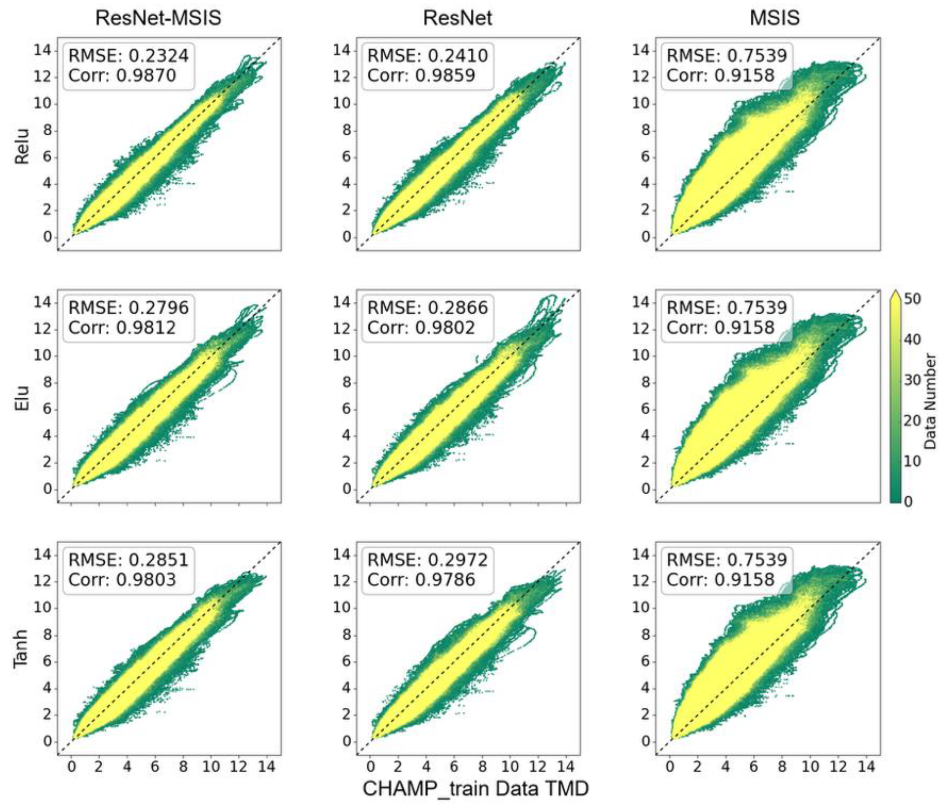
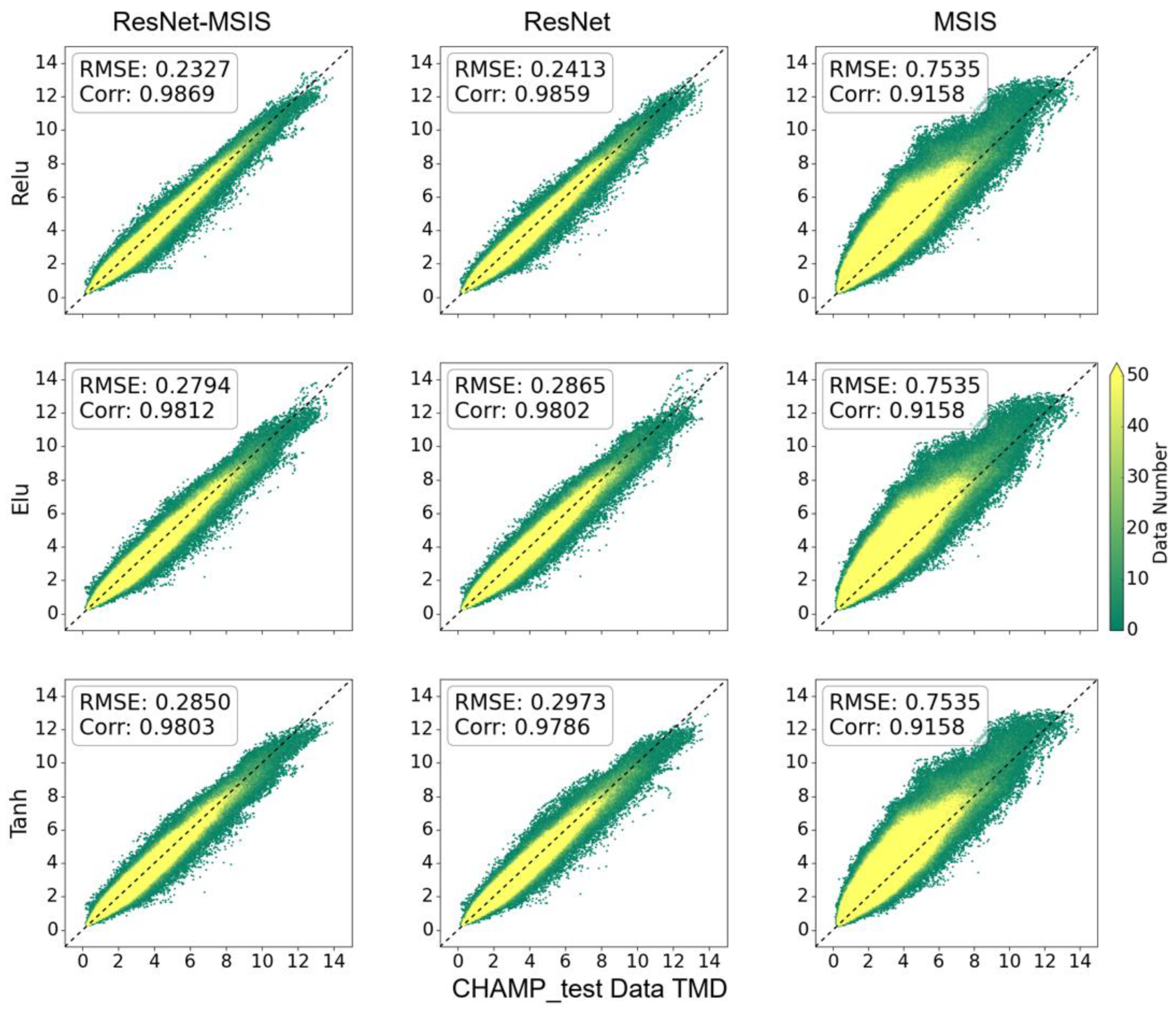
3.2. Evaluation of DL Models on Test Data
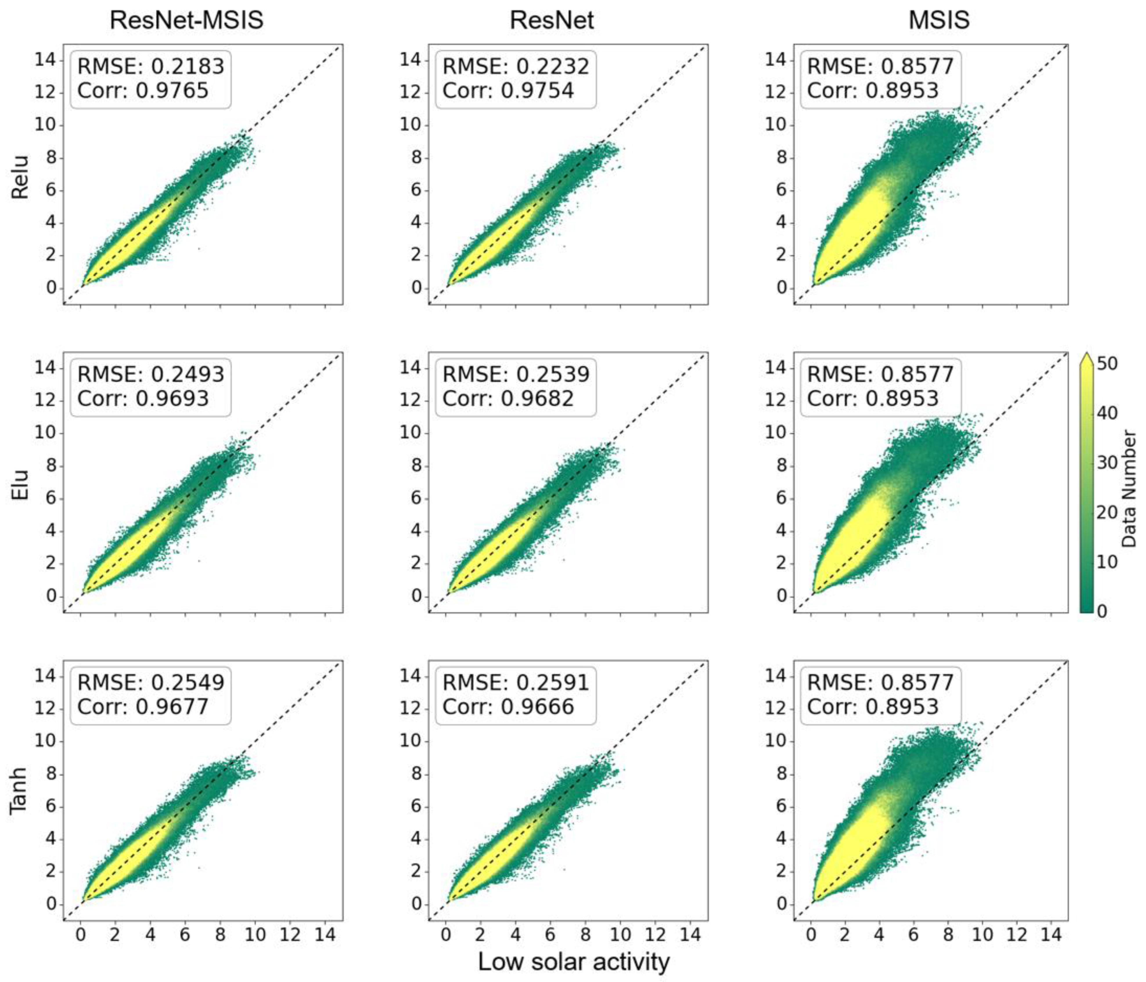
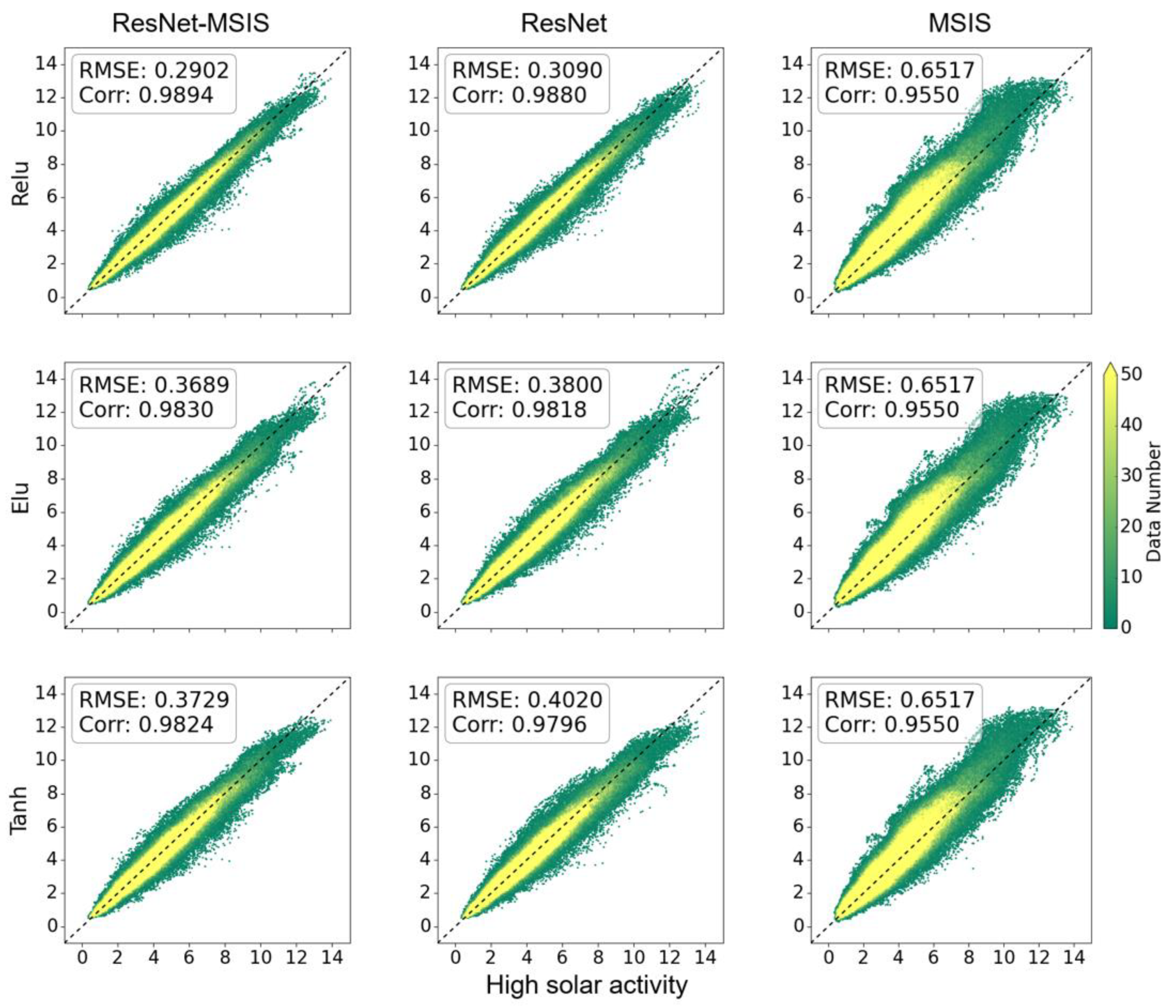
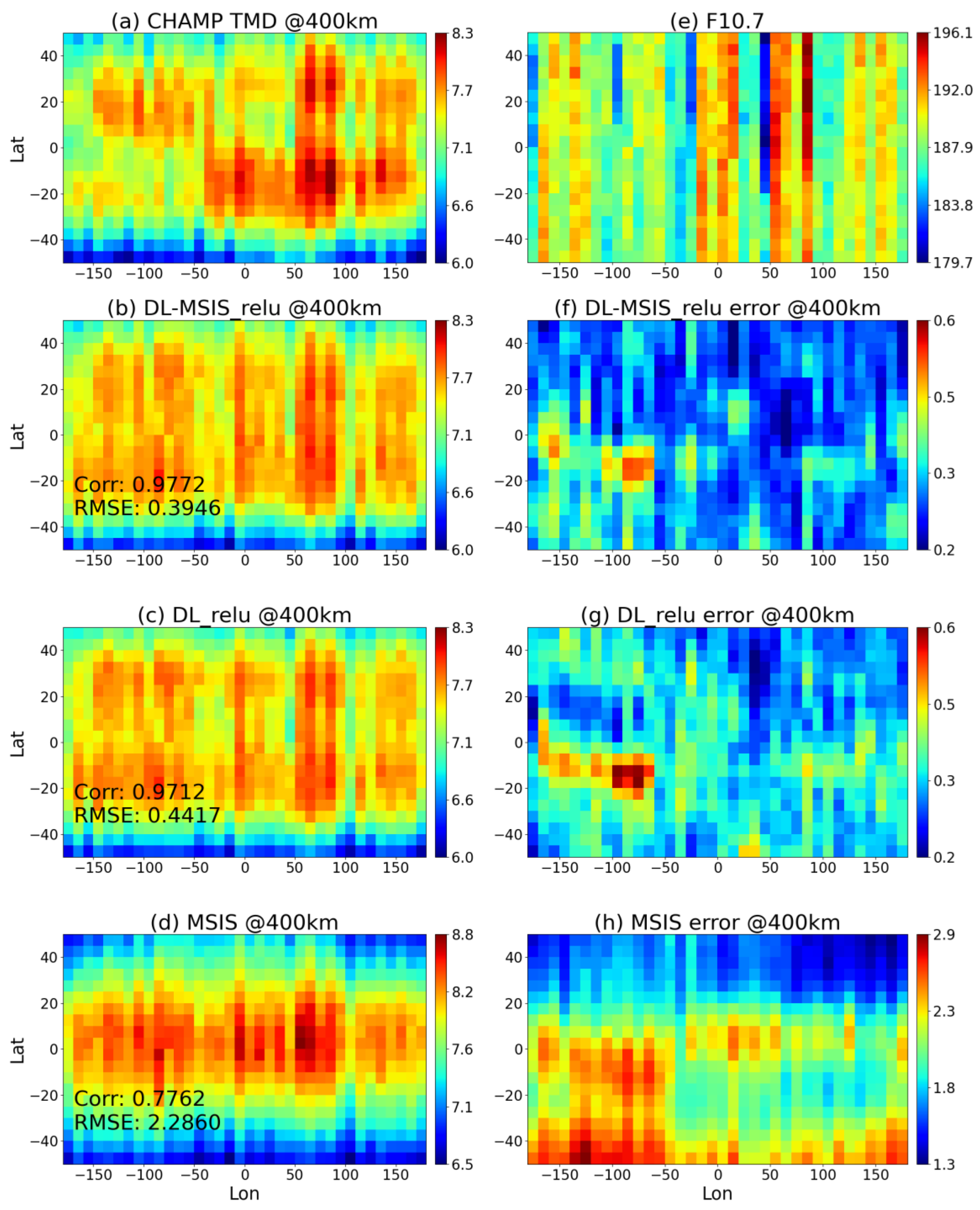
3.3. Generalization of DL Models for TMD Prediction at Different Altitudes
3.4. Evaluating DL Models for Capturing Horizontal Variations in TMD
4. Conclusions
Author Contributions
Funding
Institutional Review Board Statement
Informed Consent Statement
Data Availability Statement
Acknowledgments
Conflicts of Interest
References
- Baruah, Y.; Roy, S.; Sinha, S.; Palmerio, E.; Pal, S.; Oliveira, D.M.; Nandy, D. The loss of the Starlink satellites in February 2022: How moderate geomagnetic storms can adversely affect assets in Low-Earth orbit. Space Weather 2024, 22, e2023SW003716. [Google Scholar] [CrossRef]
- Hapgood, M.; Liu, H.; Lugaz, N. SpaceX—Sailing close to the space weather? Space Weather 2022, 20, e2022SW003074. [Google Scholar] [CrossRef]
- Dang, T.; Li, X.; Luo, B.; Li, R.; Zhang, B.; Pham, K. Unveiling the space weather during the Starlink satellites destruction event on 4 February 2022. Space Weather 2022, 20, e2022SW003152. [Google Scholar] [CrossRef]
- Berger, T.; Holzinger, M.; Sutton, E.; Thayer, J. Flying through uncertainty. Space Weather 2020, 18, e2019SW002373. [Google Scholar] [CrossRef]
- Vallado, D.A. Fundamentals of Astrodynamics and Applications, 2nd ed.; Microcosm Press: El Segundo, CA, USA, 2001; Volume 12, Available online: https://archive.org/details/FundamentalsOfAstrodynamicsAndApplications (accessed on 17 July 2024).
- Emmert, J.T. Thermospheric mass density: A review. Adv. Space Res. 2015, 56, 773–824. [Google Scholar] [CrossRef]
- Picone, J.M.; Hedin, A.E.; Drob, D.P.; Aikin, A.C. NRLMSISE-00 empirical model of the atmosphere: Statistical comparisons and scientific issues. J. Geophys. Res. Space Phys. 2002, 107, 1468–1483. [Google Scholar] [CrossRef]
- Bowman, B.; Tobiska, W.K.; Marcos, F.; Huang, C.; Lin, C.; Burke, W. A new empirical thermospheric density model JB2008 using new solar and geomagnetic indices. In Proceedings of the AIAA/AAS Astrodynamics Specialist Conference and Exhibit, Honolulu, HI, USA, 18–21 August 2008. [Google Scholar] [CrossRef]
- Bruinsma, S. The DTM-2013 thermosphere model. J. Space Weather Space Clim. 2015, 5, A1. [Google Scholar] [CrossRef]
- Emmert, J.T.; Jones, M., Jr.; Siskind, D.E.; Drob, D.P.; Picone, J.M.; Stevens, M.H.; Bailey, S.M.; Bender, S.; Bernath, P.F.; Funke, B.; et al. NRLMSIS 2.1: An Empirical Model of Nitric Oxide Incorporated Into MSIS. J. Geophys. Res. Space Phys. 2022, 127, e2022JA030896. [Google Scholar] [CrossRef]
- Bruinsma, S.; Siemes, C.; Emmert, J.T.; Mlynczak, M.G. Description and comparison of 21st century thermosphere data. Adv. Space Res. 2023, 72, 5476–5489. [Google Scholar] [CrossRef]
- Siemes, C.; Borries, C.; Bruinsma, S.; Fernandez-Gomez, I.; Hładczuk, N.; den IJssel, J.; Kodikara, T.; Vielberg, K.; Visser, P. New thermosphere neutral mass density and crosswind datasets from CHAMP, GRACE, and GRACE-FO. J. Space Weather Space Clim. 2023, 13, 16. [Google Scholar] [CrossRef]
- Panzetta, F.; Bloßfeld, M.; Erdogan, E.; Rudenko, S.; Schmidt, M.; Müller, H. Towards thermospheric density estimation from SLR observations of LEO satellites: A case study with ANDE-Pollux satellite. J. Geod. 2019, 93, 353–368. [Google Scholar] [CrossRef]
- Sutton, E.K. A new method of physics-based data assimilation for the quiet and disturbed thermosphere. Space Weather 2018, 16, e2017SW001785. [Google Scholar] [CrossRef]
- Oliveira, D.M.; Zesta, E.; Mehta, P.M.; Licata, R.J.; Pilinski, M.D.; Tobiska, K.; Hayakawa, H. The current state and future directions of modeling thermosphere density enhancements during extreme magnetic storms. Front. Astron. Space Sci. 2021, 8, 764144. [Google Scholar] [CrossRef]
- Marcos, F.A.; Kendra, M.J.; Griffin, J.M.; Bass, J.N.; Larson, D.R.; Liu, J.J. Precision low Earth orbit determination using atmospheric density calibration. J. Astronaut. Sci. 1998, 46, 395–409. Available online: https://link.springer.com/article/10.1007/BF03546389 (accessed on 22 October 2023). [CrossRef]
- Koskinen, H.E.; Baker, D.N.; Balogh, A.; Gombosi, T.; Veronig, A.; von Steiger, R. Achievements and challenges in the science of space weather. Space Sci. Rev. 2017, 212, 1137–1157. [Google Scholar] [CrossRef]
- Zhang, Y.; Paxton, L.J.; Schaefer, R.; Swartz, W.H. Thermospheric conditions associated with the loss of 40 Starlink satellites. Space Weather 2022, 20, e2022SW003168. [Google Scholar] [CrossRef]
- LeCun, Y.; Bengio, Y.; Hinton, G. Deep learning. Nature 2015, 521, 436–444. [Google Scholar] [CrossRef]
- Lee, S.; Ji, E.-Y.; Moon, Y.-J.; Park, E. One-day forecasting of global TEC using a novel deep learning model. Space Weather 2021, 19, e2020SW002600. [Google Scholar] [CrossRef]
- Liemohn, M.W.; McCollough, J.P.; Jordanova, V.K.; Ngwira, C.M.; Morley, S.K.; Cid, C.; Tobiska, W.K.; Wintoft, P.; Ganushkina, N.Y.; Welling, D.T.; et al. Model evaluation guidelines for geomagnetic index predictions. Space Weather 2018, 16, 2079–2102. [Google Scholar] [CrossRef]
- Liu, L.; Zou, S.; Yao, Y.; Wang, Z. Forecasting global ionospheric TEC using deep learning approach. Space Weather 2020, 18, e2020SW002501. [Google Scholar] [CrossRef]
- Maimaiti, M.; Kunduri, B.; Ruohoniemi, J.M.; Baker, J.B.H.; House, L.L. A deep learning-based approach to forecast the onset of magnetic substorms. Space Weather 2019, 17, 1534–1552. [Google Scholar] [CrossRef]
- Simonyan, K.; Zisserman, A. Very deep convolutional networks for large-scale image recognition. arXiv 2014, arXiv:1409.1556. [Google Scholar] [CrossRef]
- Arrieta, A.B.; Díaz-Rodríguez, N.; Del Ser, J.; Bennetot, A.; Tabik, S.; Barbado, A.; García, S.; Gil-López, S.; Molina, D.; Benjamins, R.; et al. Explainable Artificial Intelligence (XAI): Concepts, taxonomies, opportunities and challenges toward responsible AI. Inf. Fusion 2020, 58, 82–115. [Google Scholar] [CrossRef]
- Ying, X. An overview of overfitting and its solutions. J. Phys. Conf. Ser. 2019, 1168, 022022. [Google Scholar] [CrossRef]
- Pan, Q.; Wang, W.; Zhang, Y. Machine Learning Based Modeling of Thermospheric Mass Density. Space Weather 2024, 22, e2023SW003844. [Google Scholar] [CrossRef]
- Licata, R.J.; Mehta, P.M.; Tobiska, W.K.; Huzurbazar, S. Machine-learned HASDM thermospheric mass density model with uncertainty quantification. Space Weather 2022, 20, e2021SW002915. [Google Scholar] [CrossRef]
- He, C.; Li, W.; Hu, A.; Zheng, D.; Cai, H.; Xiong, Z. Thermospheric Mass Density Modelling during Geomagnetic Quiet and Weakly Disturbed Time. Atmosphere 2024, 15, 72. [Google Scholar] [CrossRef]
- Wang, P.; Chen, Z.; Deng, X.; Wang, J.; Tang, R.; Li, H.; Hong, S.; Wu, Z. The prediction of storm-time thermospheric mass density by LSTM-based ensemble learning. Space Weather 2022, 20, e2021SW002950. [Google Scholar] [CrossRef]
- Mehta, P.M.; Walker, A.C.; Sutton, E.K.; Godinez, H.C. New density estimates derived using accelerometers on board the CHAMP and GRACE satellites. Space Weather 2017, 15, 558–576. [Google Scholar] [CrossRef]
- Liu, H.; Lühr, H.; Watanabe, S. Climatology of the equatorial thermospheric mass density anomaly. J. Geophys. Res. Space Phys. 2010, 115, A12304. [Google Scholar] [CrossRef]
- Ruan, H.; Lei, J.; Dou, X.; Wan, W.; Liu, Y.C.-M. Midnight Density Maximum in the Thermosphere from the CHAMP Observations. J. Geophys. Res. Space Phys. 2013, 118, 3272–3282. [Google Scholar] [CrossRef]
- Xiong, C.; Lühr, H.; Schmidt, M.; Bloßfeld, M.; Rudenko, S. An empirical model of the thermospheric mass density derived from CHAMP satellite. Ann. Geophys. 2018, 36, 1141–1152. [Google Scholar] [CrossRef]
- Bruinsma, S.L.; Forbes, J.M. Anomalous Behavior of the Thermosphere during Solar Minimum Observed by CHAMP and GRACE. J. Geophys. Res. 2010, 115, A11323. [Google Scholar] [CrossRef]
- Covington, A.E. Solar Noise Observations on 10.7 Centimeters. Proc. IRE 1948, 36, 454–457. [Google Scholar] [CrossRef]
- Liu, H.; Hirano, T.; Watanabe, S. Empirical model of the thermospheric mass density based on CHAMP satellite observation. J. Geophys. Res. Space Phys. 2013, 118, 843–848. [Google Scholar] [CrossRef]
- Wanliss, J.A.; Showalter, K.M. High-resolution global storm index: Dst versus SYM-H. J. Geophys. Res. 2006, 111, A02202. [Google Scholar] [CrossRef]
- Staples, F.A.; Claudepierre, S.G.; Turner, D.L.; O’Brien, T.P.; Fennell, J.F. Quantifying the Role of Magnetopause and Ring Current Currents in SYM-H During Storms. Journal of Geophysical Research: Space Physics 2020, 125, e2019JA027289. [Google Scholar] [CrossRef]
- Baumjohann, W.; Kamide, Y. Hemispherical Joule heating and the AE indices. J. Geophys. Res. 1984, 89, 383–388. [Google Scholar] [CrossRef]
- Davis, T.N.; Sugiura, M. Auroral electroject activity index AE and its universal time variations. J. Geophys. Res. 1966, 71, 785–801. [Google Scholar] [CrossRef]
- Licata, R.J.; Mehta, P.M.; Weimer, D.R.; Drob, D.P.; Tobiska, W.K.; Yoshii, J. Science through machine learning: Quantification of post-storm thermospheric cooling. Space Weather 2022, 20, e2022SW003189. [Google Scholar] [CrossRef]
- Bengio, Y.; Simard, P.; Frasconi, P. Learning long-term dependencies with gradient descent is difficult. IEEE Trans. Neural Netw. 1994, 5, 157–166. [Google Scholar] [CrossRef]
- He, K.; Sun, J. Convolutional neural networks at constrained time cost. In Proceedings of the IEEE Conference on Computer Vision and Pattern Recognition, Boston, MA, USA, 7–12 June 2015; pp. 5353–5360. [Google Scholar] [CrossRef]
- He, K.; Zhang, X.; Ren, S.; Sun, J. Deep residual learning for image recognition. In Proceedings of the IEEE Conference on Computer Vision and Pattern Recognition (CVPR), Las Vegas, NV, USA, 27–30 June 2016; pp. 770–778. [Google Scholar] [CrossRef]
- Li, W.; Liu, L.; Chen, Y.; Xiao, Z.; Le, H.; Zhang, R. Improving the Extraction Ability of Thermospheric Mass Density Variations from Observational Data by Deep Learning. Space Weather 2023, 21, e2022SW003376. [Google Scholar] [CrossRef]
- Reigber, C.; Lühr, H.; Schwintzer, P. CHAMP mission status. Adv. Space Res. 2002, 30, 129–134. [Google Scholar] [CrossRef]
- Emmert, J.T. Altitude and Solar Activity Dependence of 1967–2005 Thermospheric Density Trends Derived from Orbital Drag. Journal of Geophysical Research: Space Physics 2015, 120, 2940–2950. [Google Scholar] [CrossRef]
- Lei, J.; Thayer, J.P.; Burns, A.G.; Lu, G.; Deng, Y. Wind and Temperature Effects on Thermosphere Mass Density Response to the November 2004 Geomagnetic Storm. J. Geophys. Res. Space Phys. 2010, 115, A05303. [Google Scholar] [CrossRef]
- Bezděk, A. Lognormal distribution of the observed and modelled neutral thermospheric densities. Stud. Geophys. Geod. 2007, 51, 461–468. [Google Scholar] [CrossRef]
- Kingma, D.P.; Ba, J. Adam: A Method for Stochastic Optimization. arXiv 2014, arXiv:1412.6980. [Google Scholar] [CrossRef]
- Clevert, D.-A.; Unterthiner, T.; Hochreiter, S. Fast and Accurate Deep Network Learning by Exponential Linear Units (ELUs). arXiv 2015, arXiv:1511.07289. [Google Scholar] [CrossRef]
- Glorot, X.; Bordes, A.; Bengio, Y. Deep Sparse Rectifier Neural Networks. In Proceedings of the 14th International Conference on Artificial Intelligence and Statistics (AISTATS 2011), Fort Lauderdale, FL, USA, 11–13 April 2011; Volume 15, pp. 315–323. [Google Scholar] [CrossRef]
- LeCun, Y.; Bottou, L.; Orr, G.B.; Müller, K.-R. Efficient Backprop. In Neural Networks: Tricks of the Trade; Springer: Berlin/Heidelberg, Germany, 2012; pp. 9–48. [Google Scholar] [CrossRef]
- Raissi, M.; Perdikaris, P.; Karniadakis, G.E. Physics-informed neural networks: A deep learning framework for solving forward and inverse problems involving nonlinear partial differential equations. J. Comput. Phys. 2019, 378, 686–707. [Google Scholar] [CrossRef]
- Licata, R.J.; Mehta, P.M. Uncertainty quantification techniques for data-driven space weather modeling: Thermospheric density application. Sci. Rep. 2022, 12, 7256. [Google Scholar] [CrossRef]
- Liu, H.; Yamamoto, M.; Lühr, H. Wave-4 pattern of the equatorial mass density anomaly: A thermospheric signature of tropical deep convection. Geophys. Res. Lett. 2009, 36, L18104. [Google Scholar] [CrossRef]


| Parameter Name | Parameter Value |
|---|---|
| Input 1–2: Local Solar Time (LST), in hours (h) | |
| Input 3–4: Day of Year (DoY) | |
| Input 5–6: Latitude (Lat), in degrees (°) | |
| Input 7: Altitude (Alt), in kilometers (km) | |
| Input 8–9: F10.7 and F10.7a, in solar flux units (sfu) | |
| Input 10–16: SYM-H (with the historical information), in nanoteslas (nT) | |
| Input 17–23: AE (with the historical information), in nanoteslas (nT) | |
| ), in kg/m3 | |
| Out: Thermospheric Mass Density (TMD), in kg/m3 |
| Model | Basic Environmental Parameters | Geomagnetic Indices | MSIS Density Added |
|---|---|---|---|
| ResNet | LST, DoY, Lat, Alt, F10.7, F10.7a | SYM-H, AE (with the historical information) | No |
| ResNet-MSIS | LST, DoY, Lat, Alt, F10.7, F10.7a | SYM-H, AE (with the historical information) | Yes |
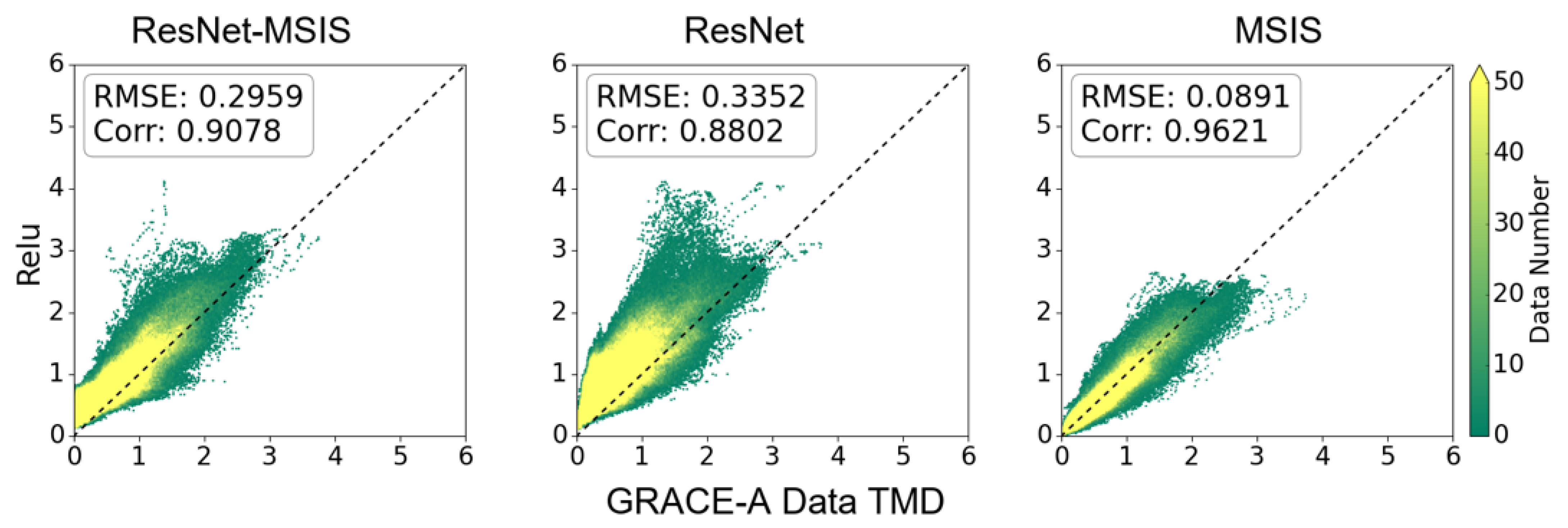
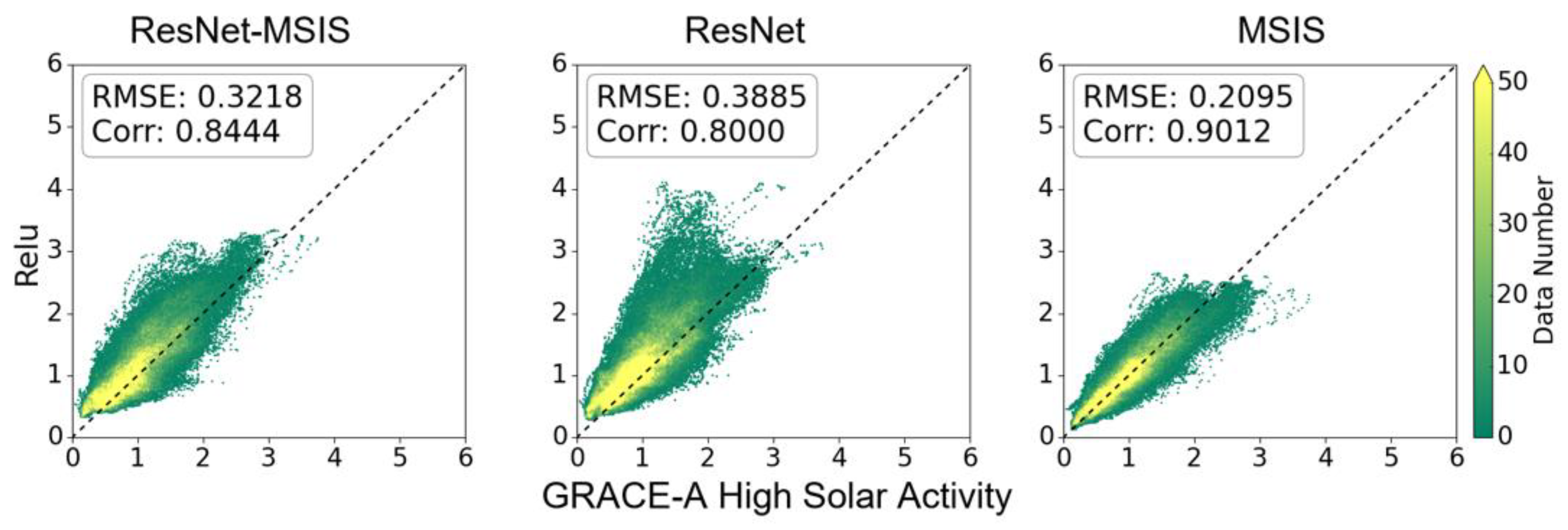
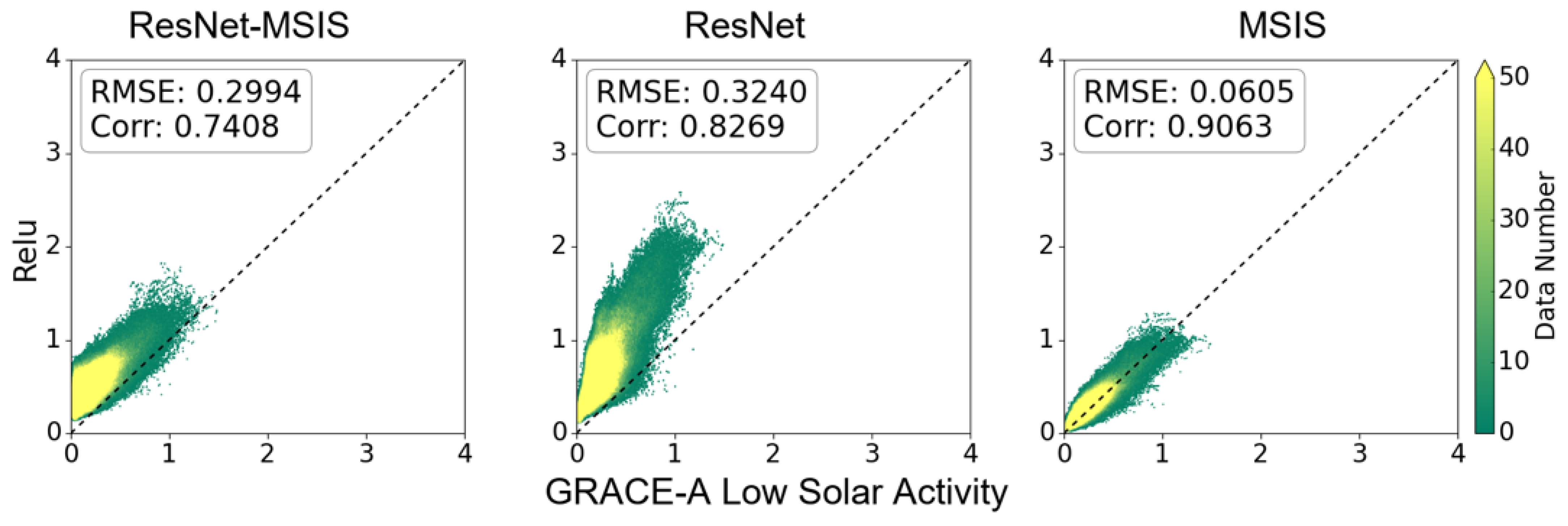
| Model | Condition | Slope (k Value) | Corr | kg/m3) |
|---|---|---|---|---|
| ResNet-MSIS_relu | Overall | 0.9415 | 0.9078 | 0.2959 |
| High solar (F10.7 > 150) | 0.7713 | 0.8444 | 0.3218 | |
| Low solar (F10.7 < 100) | 0.5901 | 0.7408 | 0.2994 | |
| ResNet_relu | Overall | 0.7456 | 0.8802 | 0.3352 |
| High solar (F10.7 > 150) | 0.6937 | 0.8000 | 0.3885 | |
| Low solar (F10.7 < 100) | 0.4190 | 0.8269 | 0.3240 | |
| MSIS | Overall | 1.0187 | 0.9621 | 0.0891 |
| High solar (F10.7 > 150) | 0.9508 | 0.9012 | 0.2095 | |
| Low solar (F10.7 < 100) | 0.8991 | 0.9063 | 0.0605 |
Disclaimer/Publisher’s Note: The statements, opinions and data contained in all publications are solely those of the individual author(s) and contributor(s) and not of MDPI and/or the editor(s). MDPI and/or the editor(s) disclaim responsibility for any injury to people or property resulting from any ideas, methods, instructions or products referred to in the content. |
© 2025 by the authors. Licensee MDPI, Basel, Switzerland. This article is an open access article distributed under the terms and conditions of the Creative Commons Attribution (CC BY) license (https://creativecommons.org/licenses/by/4.0/).
Share and Cite
Li, L.; He, C.; Zheng, D.; Li, S.; Zhao, D. A Prior Knowledge-Enhanced Deep Learning Framework for Improved Thermospheric Mass Density Prediction. Atmosphere 2025, 16, 539. https://doi.org/10.3390/atmos16050539
Li L, He C, Zheng D, Li S, Zhao D. A Prior Knowledge-Enhanced Deep Learning Framework for Improved Thermospheric Mass Density Prediction. Atmosphere. 2025; 16(5):539. https://doi.org/10.3390/atmos16050539
Chicago/Turabian StyleLi, Ling, Changyong He, Dunyong Zheng, Shaoning Li, and Dong Zhao. 2025. "A Prior Knowledge-Enhanced Deep Learning Framework for Improved Thermospheric Mass Density Prediction" Atmosphere 16, no. 5: 539. https://doi.org/10.3390/atmos16050539
APA StyleLi, L., He, C., Zheng, D., Li, S., & Zhao, D. (2025). A Prior Knowledge-Enhanced Deep Learning Framework for Improved Thermospheric Mass Density Prediction. Atmosphere, 16(5), 539. https://doi.org/10.3390/atmos16050539