Article

Spatial–Temporal Variations and Driving Factors of the Albedo of the Qilian Mountains from 2001 to 2022

School of Surveying and Land Information Engineering, Henan Polytechnic University, Jiaozuo 454003, China
*
Author to whom correspondence should be addressed.
Atmosphere 2024, 15(9), 1081; https://doi.org/10.3390/atmos15091081
Submission received: 6 August 2024 / Revised: 27 August 2024 / Accepted: 3 September 2024 / Published: 6 September 2024
(This article belongs to the Special Issue Vegetation and Climate Relationships (3rd Edition))

Abstract

:
Surface albedo plays a pivotal role in the Earth’s energy balance and climate. This study conducted an analysis of the spatial distribution patterns and temporal evolution of albedo, normalized difference vegetation index (NDVI), normalized difference snow index snow cover (NSC), and land surface temperature (LST) within the Qilian Mountains (QLMs) from 2001 to 2022. This study evaluated the spatiotemporal correlations of albedo with NSC, NDVI, and LST at various temporal scales. Additionally, the study quantified the driving forces and relative contributions of topographic and natural factors to the albedo variation of the QLMs using geographic detectors. The findings revealed the following insights: (1) Approximately 22.8% of the QLMs exhibited significant changes in albedo. The annual average albedo and NSC exhibited a minor decline with rates of −0.00037 and −0.05083 (Sen’s slope), respectively. Conversely, LST displayed a marginal increase at a rate of 0.00564, while NDVI experienced a notable increase at a rate of 0.00178. (2) The seasonal fluctuations of NSC, LST, and vegetation collectively influenced the overall albedo changes in the Qilian Mountains. Notably, the highly similar trends and significant correlations between albedo and NSC, whether in intra-annual monthly variations, multi-year monthly anomalies, or regional multi-year mean trends, indicate that the changes in snow albedo reflected by NSC played a major role. Additionally, the area proportion and corresponding average elevation of PSI (permanent snow and ice regions) slightly increased, potentially suggesting a slow upward shift of the high mountain snowline in the QLMs. (3) NDVI, land cover type (LCT), and the Digital Elevation Model (DEM, which means elevation) played key roles in shaping the spatial pattern of albedo. Additionally, the spatial distribution of albedo was most significantly influenced by the interaction between slope and NDVI.

1. Introduction

Albedo is a multifunctional Earth science parameter that holds significant importance for climate, ecosystems, natural disaster management, and global climate change research [1,2,3]. Albedo reflects the Earth’s ability to reflect solar radiation. It is the ratio of reflected radiative energy to incident radiative energy in the shortwave spectrum. Natural factors, including land cover types (LCTs) [4], vegetation [5,6], snow cover [7], land surface temperature (LST) [8], along with human activities [9,10,11,12], contribute to the spatiotemporal variations in albedo.
The Tibet Plateau is often referred to as the Earth’s “Third Pole” and exhibits susceptibility to climate shifts [13,14]. Analyzing alterations in surface albedo within this area enhances our comprehension of how climate change influences surface energy. Recent studies have indicated that the rate of climate warming on the Tibet Plateau greatly surpasses the global average [13,15], and overall, albedo has shown a decreasing trend [16]. This swift shift in climate profoundly impacts the natural environment in the plateau area and its adjacent regions, influencing atmospheric energy exchange processes [17,18].
The Qilian Mountains (QLMs), situated in the northeastern sector of the Tibet Plateau, have high elevations, complex terrain, diverse LCTs, and numerous glaciers, making them a crucial water source for the entire Northwest region. The climate changes in the Qilian Mountains are representative of those in other mountainous areas of the Qinghai-Tibet Plateau [19], making the findings of this study more broadly applicable. Albedo has a significant connection with glacier mass balance. With climate change, glaciers in regions like the Shulenan Mountains and the Tergun Mountains are continuously shrinking and losing mass [20,21], reducing albedo. This process may lead to an increase in the absorption of solar radiation by the surface [22], resulting in changes in regional surface temperature, atmospheric humidity, and downstream water resources, thereby exerting some impact on climate change.
In recent years, numerous scholars have conducted studies on the spatiotemporal distribution, variations, and determinants of surface albedo at various scales [2,23,24]. For instance, snow, with its high albedo, reflects a substantial amount of solar radiation, leading to a reduction in the energy absorbed by the Earth’s surface. Therefore, variations in snow properties (such as snow age and pollution levels) and coverage can significantly affect albedo [7,24]. Vegetation also contributes to the regulation of surface albedo. Studies have shown that the impact of deforestation and afforestation on regional climate varies by latitude. For example, deforestation may lead to a sustained temperature increase in temperate regions (0.16 ± 0.01 °C), while afforestation may have the opposite cooling effect (−0.19 ± 0.02 °C) and significantly affect albedo [25]. However, given the critical role of forests in carbon dioxide absorption and other ecological functions, the mechanisms by which these activities influence regional albedo may be more complex.
In the northeastern plains of China, the transition from grassland to cultivated land resulted in a reduction in surface albedo by 0.01–0.03. Conversely, the conversion of forests to cultivated land in the adjacent mountainous regions contributed to an increase in surface albedo by 0.005–0.015 [26]. When the albedo of artificial urban buildings increases by 0.01, each square meter of surface generates a prolonged global cooling influence of 3 × 10⁻¹⁵ K [27]. However, the interactions among various natural factors and human activities can result in alterations in albedo, and the complex interplay between them forms a mutual feedback mechanism with albedo. Hence, comprehending the primary factors and mechanisms governing the spatiotemporal features of albedo remains a complex endeavor in the examination of regional climate alterations [23].
Therefore, this study aims to achieve the following research objectives based on Moderate Resolution Imaging Spectroradiometer (MODIS) albedo products (MCD43A3) [28,29,30]: (1) analyze the multi-year temporal and spatial trends of albedo in the QLM region and explore its spatiotemporal correlations with various influencing factors; (2) study the intra-annual variation trends of albedo and its influencing factors, and analyze the temporal correlations between multi-year monthly scale anomalies and various factors; and (3) use the Geodetector model to evaluate and quantify the driving capacity of selected factors and their interactions on the spatial distribution of albedo.

2. Materials and Methods

2.1. Study Area
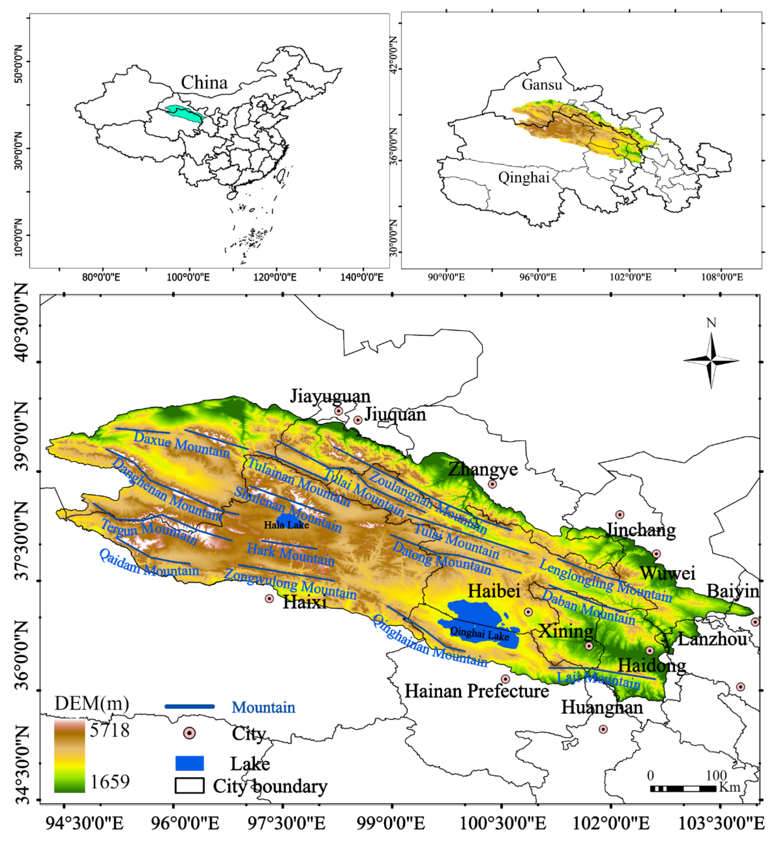
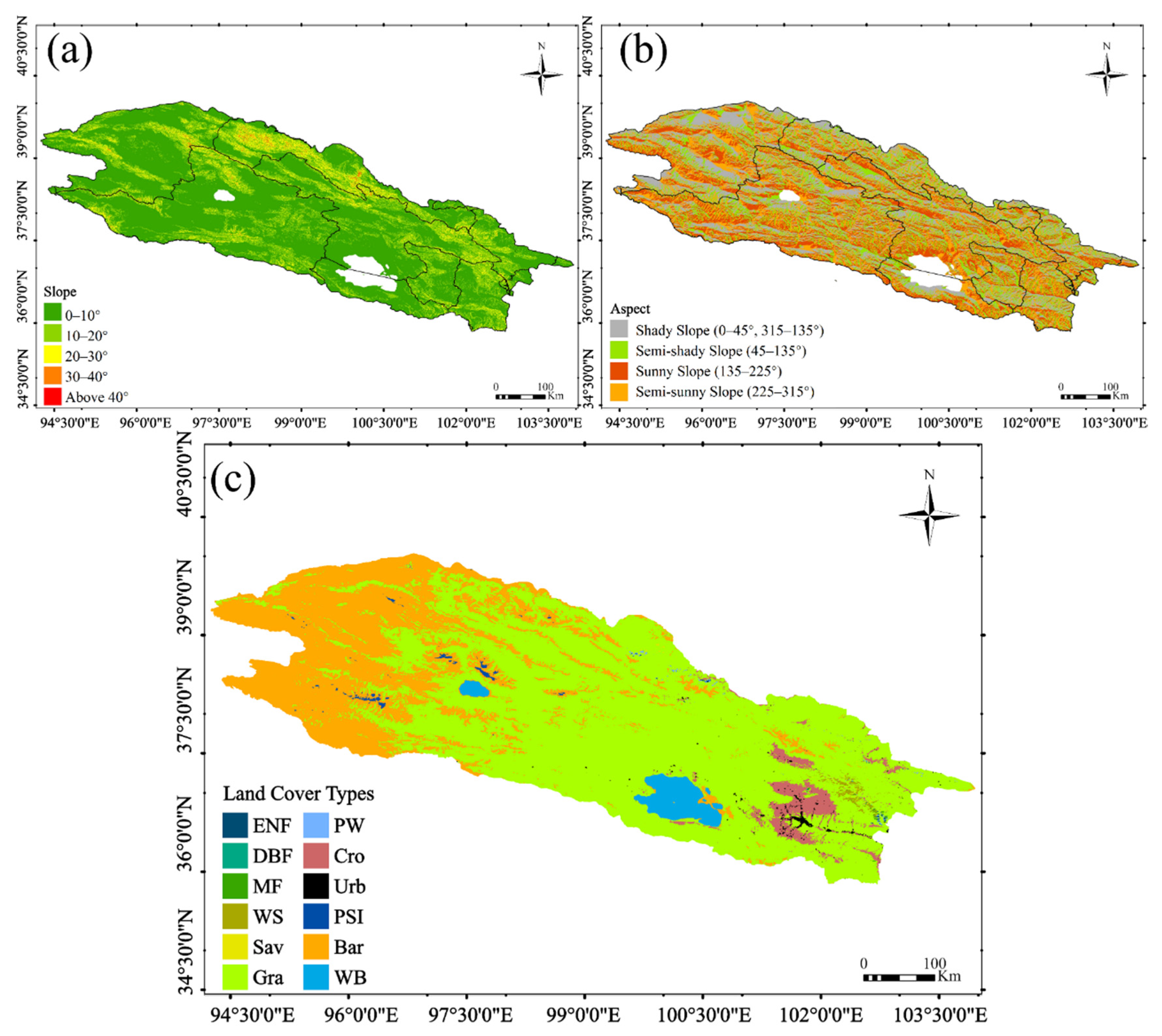
The QLMs (36–40° N, 94–104° E) are situated on the northeastern boundary of Qinghai Province and the western boundary of Gansu Province in China, representing one of the major mountain ranges within China (Figure 1). The administrative region covers 13 cities, namely Jiuquan, Jiayuguan, Haixi, Haibei, Jinchang, Hainan, Xining, Haidong, Wuwei, Baiyin, Lanzhou, Huangnan, and Zhangye. Multiple northwest-to-southeast parallel ridges and wide valleys characterize the mountain range. It spans approximately 800 km from east to west and 200–400 km from north to south, encompassing over 3000 glaciers. The QLMs serve as the headwaters for several rivers, including the Heihe, Shiyang, and Shule Rivers. The QLMs experience a gradual rise in elevation from the southwest to the northeast, with an average altitude surpassing 3600 m. Many peaks surpass 4000 m in elevation, with the highest peak being Tuánjié Peak of the Shulenan Mountains. The average slope is approximately 8° (Figure 2a), and the Shady slope accounts for 28.6% (Figure 2b). Encompassing 12 stable LCTs, the QLMs are dominated by grasslands (64.80%) and barren land (28.77%), which together cover 93.57% of the region (Figure 2c).
Figure 1. Geographic location and elevation of the QLMs.
Atmosphere 15 01081 g001
Figure 2. (a) Slope, (b) aspect, and (c) land cover types of the QLMs (the explanation of the abbreviation is included in Table 1).
Atmosphere 15 01081 g002

2.2. Data

This study predominantly used remote sensing products (Table 2), which encompassed MODIS albedo, LST, NSC for quantifying snow cover, and NDVI. Furthermore, the Shuttle Radar Topography Mission (SRTM) elevation data was represented using DEM and was also utilized to compute the slope and aspect information for the QLMs.

Data Preprocessing

Considering that solar radiation energy is predominantly concentrated in the shortwave spectrum [31], we used the MODIS MCD43A3 daily scale reflectance dataset for the shortwave band from 2001 to 2022. This dataset includes both black-sky albedo ( B S A ) and white-sky albedo ( W S A ). Subsequently, we calculated the authentic surface albedo using a linear weighted formula (Equation (1)) [32,33].
A l b e d o = s × W S A + 1 s × B S A
In Equation (1), s represents the sky diffuse fraction, which signifies the ratio of scattered light in the sky to the total radiation. This factor reflects the contribution of atmospheric scattering to the overall radiation. The specific value of the sky diffuse fraction varies based on geographic location, season, weather conditions, and atmospheric characteristics. This study adopts the constant value of 0.2 as the sky diffuse fraction (s) for calculating the actual surface albedo [34].
This study prepared daytime MODIS LST (MOD11A1 LST, 1 km) [35,36], 16-day MODIS NDVI products (MOD13A1, 500 m) [37], annual MODIS land cover products (MCD12Q1, 500 m) [38,39], and daily snow cover products (MOD10A1, 500 m) [40,41] to elucidate some of the ecological factors contributing to changes in albedo. These products underwent preprocessing using Google Earth Engine [42,43,44,45], including resampling, and removal of invalid data points. Additionally, elevation data were used to compute slope and aspect data. Python, MATLAB, and ArcGIS Pro were used to analyze and validate the preprocessed data.
All MODIS products are based on the WGS84 geographic coordinate system, and data for LST, elevation, slope, and aspect were adjusted to 500 m resolution through nearest-neighbor interpolation. All products were monthly and yearly averaged using the mean aggregation method to enable the analysis of albedo fluctuations and their associations with NDVI, LST, and NSC. By synthesizing the MCD12Q1 LCT products for a total of 22 years from 2001 to 2022 using the mode method, the perennial and stable LCTs of the QLMs were obtained. A basic statistical analysis was also performed on the multi-year variations of the average elevation and area proportion corresponding to the permanent snow and ice regions (PSI).
Using geographic detectors to assess the influence of various factors on albedo, we discretized continuous variables, including elevation, slope, NSC, NDVI, and LST, using the natural breakpoint method, dividing them into five categories. The slope aspect was categorized into four natural zones: semi-shady slope (45–135°), sunny slope (135–225°), semi-sunny slope (225–315°), and shady slope (0–45°, 315–360°). From 2001 to 2022, we selected five years: 2001, 2006, 2011, 2016, and 2021. We conducted a systematic sampling within the QLM region and removed points with missing values, resulting in approximately 29,125 sampling points.

2.3. Methods

2.3.1. Theil–Sen Median Trend Analysis

The Theil–Sen median method, also known as Sen’s slope (SS) estimation, represents a robust non-parametric statistical approach for assessing trends [46,47]. Compared with other methods, it is less susceptible to the influence of data noise interference. Given the uncertain distribution and fluctuations of annual mean albedo, this method is well-suited for calculating albedo trends. The SS is determined through calculations involving permutations and combinations of the various time points within the time series, and the SS is derived by taking the median of the resultant slopes. Taking albedo as an example, the formula for calculating SS is as follows:
S S = m e d i a n A l b e d o i A l b e d o j i j         2001 j i 2022
In the equation, a positive SS indicates a rising albedo trend over the time series, whereas a negative SS signifies a declining trend.

2.3.2. Mann–Kendall Method

The Mann–Kendall method is a non-parametric technique based on statistical theory, used to assess the significance of trends in time series data without the requirement for the data to follow a normal distribution [48,49,50]. For albedo as an example, it is computed as follows:
S = k = 1 n 1 j = 1 n S g n A l b e d o j A l b e d o k
S g n A l b e d o j A l b e d o k = + 1 ,   ( A l b e d o j A l b e d o k ) > 0 0 , ( A l b e d o j A l b e d o k ) = 0 1 , A l b e d o j A l b e d o k < 0
V a r S = n n 1 2 n + 5 i = 1 m t i ( t i 1 ) ( 2 t i + 5 ) 18
Z = S 1 V a r S ,   S > 0 0 ,   S = 0 S + 1 V a r S ,   S < 0
In Formulas (3) and (6), the time series length is n, A l b e d o k , and A l b e d o j representing the albedo values for the k and j years, respectively, where k and j are not equal and both do not exceed n. In this study, n = 22, and m denotes the number of tied groups. In Formula (4), the sign function sgn is used to indicate the sign of a value. In Formula (5), t i represents the albedo data for the i-th year. The statistic Z spans a range of ( , + ) . Taking 0.05 as the significance level α , and comparing the absolute value of the statistic with the critical value u 1 α 2 to assess significance, when Z > u 1 α 2 , rejecting the null hypothesis indicates a significant change in the time series. Therefore, in this study, we choose Z > 1.96 as the criterion for determining that the studied time series has changed significantly.

2.3.3. Anomaly

Due to the significant intra-annual variations in meteorological factors, the mean monthly values differ. To facilitate the comparison of changes over multiple years at the same level, this study uses the albedo in conjunction with monthly anomalies of various factors to explore the relationships among different meteorological elements [51,52]. The calculation formula is as follows:
A n o m a l y = x t x ¯ t ,         1 t 12
In the context of this study, x ¯ t represents the average albedo for the month t over the years 2001 to 2022, while x t signifies the average albedo value for the month t .

2.3.4. Geographical Detector

Geographical detectors (Geodetectors) are an innovative spatial statistical approach employed to unveil spatial disparities and investigate driving factors [53,54,55]. It comprises four components: factor detection, interaction detection, ecological detection, and risk detection, with this study mainly focusing on the first three.
(1) Factor detection. This section intends to uncover the spatial distribution features of albedo in the QLMs and gauge the explanatory power (q value) of different factors in explaining the spatial distribution of albedo. It is expressed as follows:
q = 1 h = 1 L N h σ h 2 N σ 2 = 1 S S W S S T
S S W = h = 1 L N h σ h 2 ,     S S T = N σ 2
In the provided formula, y denotes the dependent variable (albedo), and x represents the influencing factors. h = 1 , 2 , , L represents the stratification (strata) of y or x, which refers to classification or partitioning. The number of units in the entire region and within stratum h is represented as N and N h , respectively. The variance of y for the entire region and within stratum h is denoted by σ 2 and σ h 2 , respectively. The total sum of squares for the entire region and the sum of squares within strata are represented as SST and SSW, respectively. The q value ranges from 0 to 1, with higher q values indicating greater explanatory power of x for y and a more pronounced influence on spatial variations.
(2) Interaction detection. Taking two influencing factors, x 1 and x 2 , as an example, we calculate their individual and interactive explanatory power on y, denoted as q ( x 1 ) , q ( x 2 ) , and q ( x 1 x 2 ) . By evaluating these q values, we assess whether the explanatory power of the spatial distribution of y is enhanced, weakened, or remains independent under the synergy of two factors (Table 3). When q x 1 x 2 > M a x ( q x 1 , q x 2 ) , it is determined as a two-factor enhancement. If q x 1 x 2 > q x 1 + q x 2 , it is identified as a nonlinear enhancement. When q x 1 x 2 falls between the explanatory power of the two individual factors, or is less than the minimum of the two, it is classified, respectively, as single-factor nonlinear attenuation or nonlinear attenuation. It is noteworthy that if q x 1 x 2 equals the sum of the two individual explanatory powers, the two factors are considered independent in explaining the spatial distribution of y.
(3) Ecological detection. Utilizing the F-statistic test (Fisher’s criterion), it examines the significance of differences in the spatial distribution impact of x 1 and x 2 on y in the interaction analysis:
F = N x 1 N x 2 1 S S W x 1 N x 2 N x 1 1 S S W x 2
S S W x 1 = h = 1 L 1 N h σ h 2 ,   S S W x 2 = h = 1 L 2 N h σ h 2
In the above formulas, N x 1 and N x 2 represent the sample sizes for factors x 1 and x 2 , respectively. The sum of within-group variances formed by x 1 and x 2 is denoted by S S W x 1 and S S W x 2 , respectively. The number of strata or tiers for x 1 and x 2 is denoted by L1 and L2, respectively. Rejecting the null hypothesis H 0 ( S S W x 1 = S S W x 2 ) at significance level α indicates a significant difference in the spatial distribution impact of these two factors on y.

3. Results

3.1. Temporal and Spatial Variations of Albedo

Annual Spatiotemporal Variation of Albedo

The average albedo of the QLMs from 2001 to 2022 was approximately 0.204. Higher albedo values are predominantly observed in the northwest region of the mountain range (Figure 3a), such as the Tergun Mountains, and the southern part of the Shulenan Mountains adjacent to Lake Hala. These areas exhibit spatial correspondence with higher NSC and lower LST values (Figure 3d). The albedo in these regions tends to stay above 0.4 due to their perennial snow and ice coverage, substantial glacier reserves, and lower NDVI values (Figure 3c), which indicate predominantly bare soil. In contrast, the southeastern part of the QLMs shows lower albedo values, higher NDVI values, moderate LST, and lower NSC levels, resulting in albedo values consistently below 0.2 throughout the years.
From 2001 to 2022, the annual average albedo of the QLMs fluctuated within the range of 0.18–0.24. The Sen’s Slope for albedo was −0.0004, indicating a subtle decreasing trend (Figure 4a). Notably, the lowest and highest albedo values were observed in 2019 and 2022, respectively, with a substantial variation in albedo between 2018 and 2022. The SS for NSC was −0.0508, also exhibiting a weak decreasing trend, which was significantly consistent with albedo changes (R = 0.975, Pearson correlation coefficient, the same applies to the following). In 2019, both NSC and the proportion of PSI reached their maximum values, attributed to extensive snow disasters in Qinghai and Gansu provinces. Heavy snowfall affected multiple areas in Qingnan Pasture, resulting in the highest number of severe snowfall stations since 1961. Consequently, albedo and NSC significantly increased in 2019.
From 2001 to 2022, the PSI in the QLMs exhibited a marginal upward trend, with the corresponding average elevation of PSI also showing a slight increase (SS = 1.3396) (Figure 4d). This observation suggests a potential rise in the high-altitude snowline, leading to increased melting of high-altitude glaciers and snow. This phenomenon partly explains the significant and relatively rapid increase in the NDVI with an SS of 0.0018 (Figure 4b). Over the 22 years, the QLMs gradually became greener, as evidenced by the negative correlation (R = −0.210) between vegetation changes and annual albedo variations. Meanwhile, the LST in 2022 increased by 0.069 K compared with 2001, showing a marginal overall increase with an SS of 0.0056 (Figure 4c). This change affected plant growth and contributed to the decrease in NSC in the QLMs, ultimately having a significant negative influence on albedo changes (R = −0.478). In summary, although vegetation dynamics and surface temperature influenced albedo, the high reflectance property of snow remained the decisive factor determining the overall albedo variations in the QLMs over the 22 years.
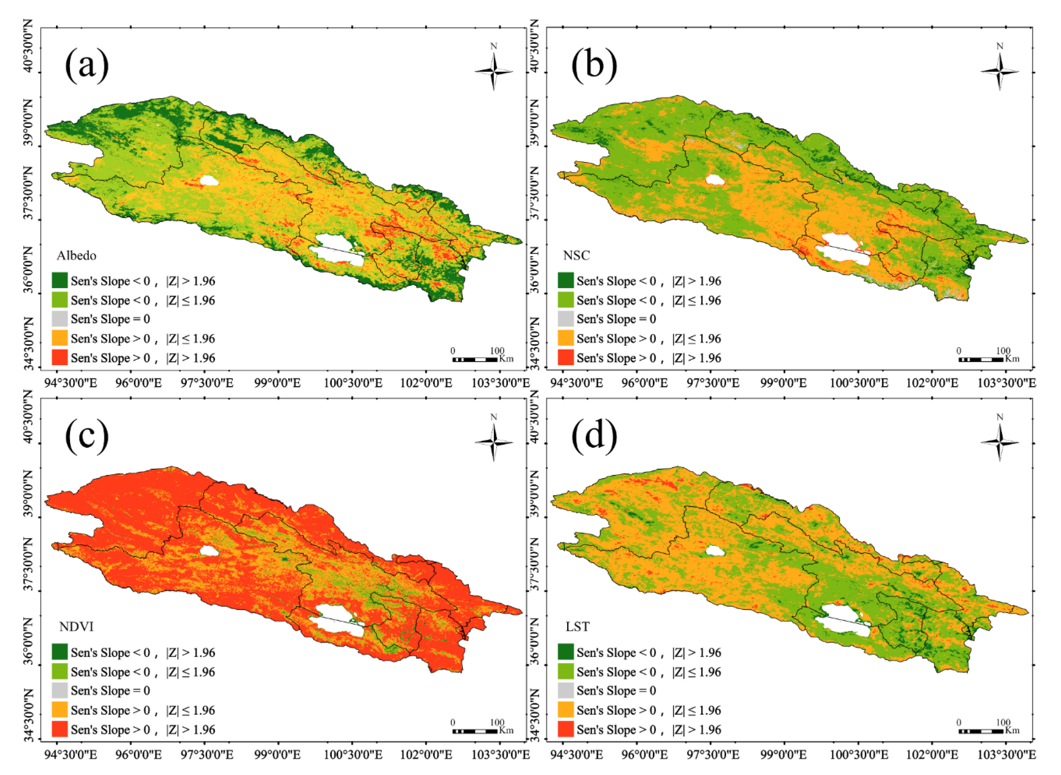
Approximately 22.8% of the QLMs exhibited significant changes in albedo (Figure 5a). Among these, 17.5% of the regions showed significant decreases, including glacier-rich mountain areas such as the Laji Mountains, Qinghainan Mountains, Shulenan Mountains, Danghenan Mountains, and Zoulangnan Mountains. About 5.3% of the regions, including the Daban Mountain range, experienced significant increases. It is noteworthy that the albedo changes in most areas of the central QLMs were not significant, which was related to the stable grassland cover in this area (Figure 2c). Additionally, compared to other regions, the NSC changes in this area were also not significant (Figure 5b).
In the QLM region, NSC significantly decreased in approximately 3.79% of the area, while 1.84% of the area experienced a significant increase in NSC, showing a distribution pattern similar to the areas with significant changes in albedo. Notably, both NSC and albedo exhibited a significant upward trend in the mountainous areas southwest of Qinghai Lake and at the junction of Haibei and Xining.
For NDVI in the QLMs, approximately 0.77% of the regions exhibited significant decreases (Figure 5c), while 66.32% experienced significant increases. The increased NDVI was distributed throughout the QLMs, with a prominent concentration in Jiuquan. This indicates that there has been a substantial improvement in vegetation cover and health in the region over the past 22 years. Only a small portion of the northern area near Qinghai Lake did not show significant changes.
Regarding LST in the QLMs, approximately 2.77% of the regions experienced significant decreases (Figure 5d), primarily concentrated in Xining City. Approximately 2.33% of the regions showed significant increases, located in the northern part of Jiuquan. The majority of the regions did not display significant changes.

3.2. Correlation between Albedo and the Monthly Anomalies of LST, NSC, and NDVI

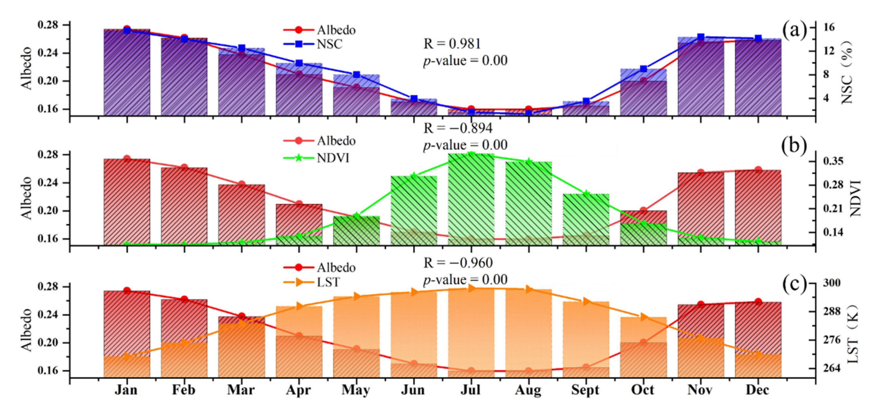
Based on the characteristics of the 22-year monthly average albedo variations in the QLMs, the analysis revealed that the monthly variations in albedo throughout the year typically fell within the range of 0.16 to 0.27. The highest values were observed in January, while the lowest occurred in August (Figure 6).
By comparing the multi-year monthly average values of albedo with NSC, NDVI, and LST in the QLM region, it was found that the intra-annual variation trend of albedo was highly similar to that of NSC, with a significant positive correlation (correlation coefficient of 0.981). Seasonal changes in snow cover caused fluctuations in snow albedo, which significantly affected the interannual variation of albedo. Albedo showed a significant negative correlation with both NDVI and LST, with correlation coefficients of −0.894 and −0.960, respectively. The variations in vegetation growth during different seasons and fluctuations in surface temperature influenced the dynamics of snow and glaciers. These factors collectively contributed to the seasonal characteristics of the surface, ultimately leading to the seasonal variation in albedo.
Between 2001 and 2022, the monthly albedo anomalies of the QLMs exhibited significant seasonal dependence and correlations with NSC, NDVI, and LST anomalies at the monthly time scale (Figure 7). Among these, the peak anomalies for albedo occurred in January 2019 and 2020, measuring 0.11 and 0.13, respectively.
Over the 22 years, a strong positive correlation of 0.956 was observed between albedo anomalies and NSC monthly anomalies in the QLMs. From September 2015 to October 2018, most months exhibited negative NSC anomalies, indicating a greater reduction in snow cover during these periods. Conversely, from November 2018 to May 2021, most months showed positive NSC anomalies, suggesting a recovery in snow cover. The albedo was significantly influenced by the abnormal variations in snow cover in the QLMs. The increase and decrease in snow significantly affected the snow cover area and snow density, thereby driving the monthly albedo anomalies. This underscores the importance of snow cover in the climate and ecosystem of high-altitude regions.
A negative correlation, with a coefficient of −0.618, was observed between albedo and NDVI monthly anomalies. From 2015 to 2022, in most months, especially during the summer, significant positive anomalies were observed. This indicates that during this period, vegetation growth in the summer months was particularly pronounced, implying a long-term trend of vegetation recovery. Simultaneously, during this period, NSC showed higher positive anomalies in winter, while LST exhibited positive anomalies in spring and summer. These conditions likely led to increased soil moisture during the growing season, promoting vigorous vegetation growth.
A significant inverse relationship was found between albedo and LST monthly anomalies, with a correlation coefficient of −0.574. Over the 22 years, LST anomalies exhibited substantial fluctuations, indicating considerable variations in surface temperature across different months in the QLMs. Because both vegetation and snow cover undergo seasonal variations and influence LST, this effect is readily observable on a monthly scale. Additionally, the seasonal variations in LST also to some extent affect albedo, snow cover, and vegetation.

3.3. Driving Factors for the Albedo Spatial Distribution

3.3.1. Single-Factor and Significant Difference Analysis

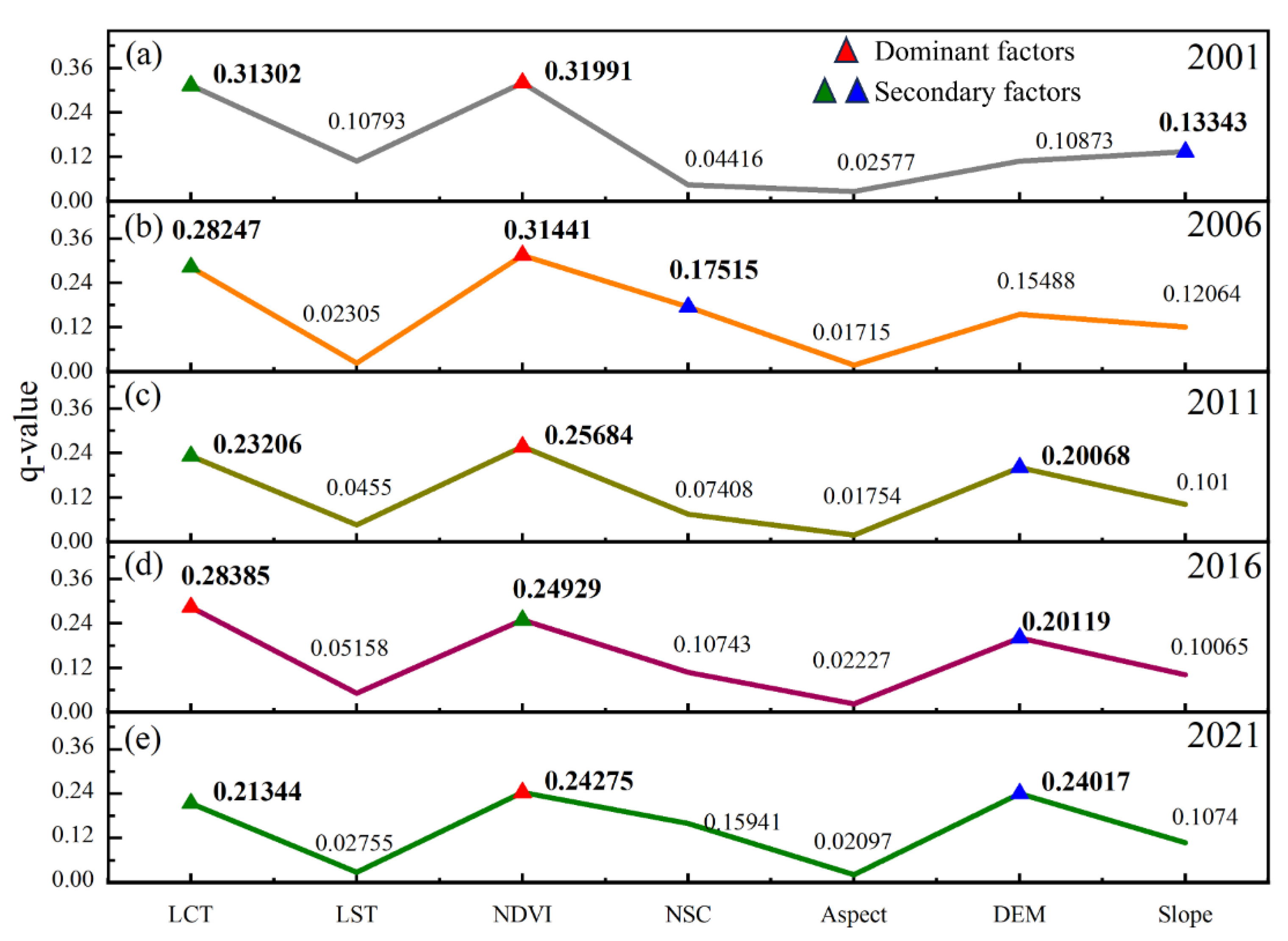
We selected five years, namely 2001, 2006, 2011, 2016, and 2021, to analyze the effects of selected factors on the spatial distribution pattern of albedo in the QLMs using geographical detectors (Figure 8). The results of factor detection indicated that different factors had varying degrees of explanatory power on the spatial distribution of albedo in the QLMs. Among these factors, NDVI, LCT, and DEM were identified as significant determinants of the spatial distribution pattern of albedo in this region. However, the effect of the aspect was found to be statistically insignificant. In the geographical detector analysis, we also used ecological detection to assess if different driving factors significantly influence the spatial distribution of albedo in the QLMs (Figure 9).

3.3.2. Analysis of Factors Interaction

Through the interaction detector analysis, we found that among the 21 pairs of interactions between seven factors in the spatial pattern of albedo in the QLMs (Figure 10), indicating that the interaction between slope and NDVI played a crucial role in influencing the spatial patterns of albedo in the QLMs, with an explanatory power exceeding 48%. Similarly, the average explanatory power between LST and DEM also exceeded 43%. The interactions between NDVI and DEM, LCT and slope, as well as NSC and slope, all exhibited an average explanatory power exceeding 40%. However, it was worth noting that the average explanatory power of LST and aspect was only 0.092, and the interaction between them was not significant. Furthermore, the average explanatory power for other interaction types among factors was above 14%. These findings suggest that the explanatory power involving interactions between two factors surpasses that of any single factor alone, and these interactions demonstrate non-linear enhancement and synergistic effects. This indicates the absence of single-factor non-linear attenuation, single-factor enhancement, and independent effects of individual factors.

4. Discussion

In the past few decades, against the backdrop of global warming, different regions experienced varying climate changes [56,57]. The issue of ecological environmental changes in the QLMs attracted close attention from the Chinese government, leading to a series of rectification measures [58]. In this context, changes in the ecological environment of the QLMs have drawn close attention from the Chinese government, which has implemented corresponding ecological incentive policies and subsidies. Examples of such initiatives include the “Three-North Shelterbelt Project”, initiated in 1979 [59,60], and the “Grain for Green Program”, launched in 1999 [61,62]. The environment in the QLMs gradually stabilized, leading to significant ecosystem restoration [63,64].
Under the combined influence of climate change and human activities, between 2001 and 2022, the entire QLMs witnessed a significant increase in NDVI (normalized difference vegetation index), indicating a widespread enhancement in vegetation coverage. Concurrently, surface temperatures exhibited an upward trend, and albedo and NSC (normalized difference snow index snow cover) exhibited a declining trend. This trend aligns with the changes in NDVI observed in the Tibet Plateau, suggesting an overall increase in vegetation coverage [65,66]. Plants often seek suitable growth conditions and may migrate to higher altitudes, and previous studies have indicated that the pace of this migration is gradually accelerating [67]. However, without sufficient water resources, this can also result in drought and water scarcity. Additionally, some plants may struggle to adapt to climate change in their original habitat, leading to population declines.
Lower albedo can lead to increased absorption of solar energy by the Earth’s surface, accelerating global warming [68]. The temporal correlation between albedo and NSC in the QLMs was evident, and snow was the primary factor driving albedo changes in the QLMs. Snow albedo was influenced by various factors, including LST (Land surface temperature), snow depth, precipitation, snowmelt, and pollutants such as black carbon. These factors altered the structure and optical properties of the snow. Higher LST led to more snowmelt, exacerbating global climate change [69]. Increased snow depth typically raised albedo, while shallower snow layers often reduced albedo as they absorbed more solar radiation [70]. Rainfall and snowmelt altered the snow surface, also affecting albedo [71,72]. Pollutants like black carbon could adhere to the snow surface, absorbing solar radiation and causing rapid melting, reducing coverage and depth, thereby impacting albedo [73]. Complex interactions among these factors might have resulted in varying degrees of influence across different seasons and regions.
However, according to the results from the geographical detector analysis, it seems that NSC was not the primary influencing factor for the spatial distribution of albedo in the QLMs. This might be because regions with PSI (permanent snow and ice regions) make up only a small proportion. Although the permanent ice and snow-covered area exhibited a slightly increasing trend, it was not statistically significant. Additionally, the corresponding mean elevation of the permanent snow-covered regions was on the rise.
In contrast, NDVI did not exhibit a significant temporal correlation with albedo variations on an annual scale. Nevertheless, the geographical detector analysis indicated that among the factors selected in this study, NDVI emerged as the primary driver influencing the spatial distribution of albedo. Spatially, the higher negative correlation values between NDVI and albedo were primarily concentrated in the northwestern region where the barren meets the grassland. This suggested that albedo was more responsive to lower NDVI values. Although the geographical detector verified the significant influence of NDVI on albedo’s spatial distribution, the effect of vegetation during non-growing and growing seasons might have differed, requiring further in-depth investigation [74]. Amid the backdrop of warming and moistening in the high-altitude regions, changes in LCTs (land cover types) also significantly drove variations in surface albedo and its spatial distribution, thereby exerting a substantial influence on the regional climate.
This study also has certain limitations. The accuracy of the snow component (snow albedo) in the MCD43A albedo product was slightly lower than that of soil and vegetation canopy albedo [75,76]. By integrating existing station data in the QLMs or through further calibration, it may be possible to more accurately capture the influence of various snow properties on albedo changes. For simplification, a constant value of 0.2 was selected for the sky scattering factor when linearly weighing WSA and BSA to calculate the actual albedo. However, the sky scattering factor is a complex parameter influenced by various factors, including geographical location, time, season, weather conditions, and atmospheric constituents. A more comprehensive consideration of these factors could be a deeper exploration of the patterns of surface albedo changes.
The geographic detector analysis used a natural classification method to discretize continuous variables without using other methods. Different discretization methods may yield distinct detection results.
This study selected only seven natural factors as driving factors influencing the spatial distribution of albedo in the QLMs. It did not account for other factors such as soil moisture [77]; precipitation [78,79]; atmospheric aerosols, water vapor, and cloud cover [80,81]; or surface roughness [82,83]. Furthermore, anthropogenic factors such as buildings and structures, roads, urbanization [27], and land use for industrial activities have not been considered. Natural and anthropogenic factors interact and collectively shape the spatial distribution and changes in albedo. When studying albedo, considering anthropogenic factors is crucial, particularly in urbanized areas and regions with frequent human activities.

5. Conclusions

From 2001 to 2022, the spatial distribution of albedo in the QLMs exhibited a gradual increase from southeast to northwest. Approximately 22.8% of the region experienced significant changes, with a slight overall decrease in albedo. The seasonal fluctuations of NSC (normalized difference snow index snow cover), LST (Land surface temperature), and vegetation collectively influenced the overall albedo changes in the QLMs. Albedo exhibited highly similar trends and significant correlations with NSC across interannual monthly variations, multi-year anomalies, and regional multi-year average trends, indicating that changes in snow albedo, as reflected by NSC, played a major role. Additionally, the slight increase in the area proportion and average elevation of permanent snow and ice regions (PSI) in the QLMs may suggest a gradual upward shift of the high mountain snowline on the plateau.
In this study, the influence of various factors on the spatial pattern of albedo was ranked below according to their degree of impact: NDVI (normalized difference vegetation index) > LCT (land cover type) > DEM (Elevation) > Slope > NSC > LST > Aspect. Notably, NDVI and LCT each played significant roles in shaping the spatial pattern of albedo, with NDVI being the dominant factor. Interactions between these factors enhanced their explanatory power on albedo spatial distribution, exhibiting both linear and nonlinear effects. The non-linear enhanced interaction between slope and NDVI exhibited the highest explanatory power, with an average explanatory power of 52.2%. In contrast, the interaction between LST and aspect had the lowest explanatory power, averaging less than 10%.
The overall NDVI in the QLMs demonstrated a significant upward trend with SS of 0.00178. Furthermore, from the spatial perspective, there was a significant increasing trend in NDVI in over 66% of the areas. This suggested that the QLMs were gradually becoming greener. The decreasing trend in albedo led to rising surface temperatures, reduced snow cover, or changes in snow characteristics in the past. Ultimately, this exacerbated climate warming and, to some extent, influenced the growth, recovery, and migration of vegetation.

Author Contributions

H.X.: Methodology, Investigation, Software, Formal analysis, Conceptualization. H.Z.: Writing—original draft, Methodology, Investigation, Software, Formal analysis, Conceptualization. Z.Y.: Writing—review and editing, Methodology, Investigation. Q.M.: Writing—review and editing, Methodology, Supervision. H.W.: Data curation, Investigation. Z.L.: Visualization. All authors have read and agreed to the published version of the manuscript.

Funding

This research was funded by the Key Scientific and Technological Project of Henan Province (No. 232102320247).

Institutional Review Board Statement

Not applicable.

Informed Consent Statement

Not applicable.

Data Availability Statement

All MODIS products and SRTM data used in this study can be downloaded from Google Earth Engine, and detailed URLs for data sources are provided in Section 2.2 (Data). All data used are from publicly available datasets.

Conflicts of Interest

The authors declare no conflicts of interest.

References

  1. Gao, F.; Schaaf, C.B.; Strahler, A.H.; Roesch, A.; Lucht, W.; Dickinson, R. MODIS bidirectional reflectance distribution function and albedo Climate Modeling Grid products and the variability of albedo for major global vegetation types. J. Geophys. Res. Atmos. 2005, 110, D01104. [Google Scholar] [CrossRef]
  2. Wielicki, B.A.; Wong, T.M.; Loeb, N.; Minnis, P.; Priestley, K.; Kandel, R. Changes in Earth’s albedo measured by satellite. Science 2005, 308, 825. [Google Scholar] [CrossRef] [PubMed]
  3. Zhang, X.; Liang, S.; Wang, K.; Li, L.; Gui, S. Analysis of Global Land Surface Shortwave Broadband Albedo From Multiple Data Sources. IEEE J. Sel. Top. Appl. Earth Obs. Remote Sens. 2010, 3, 296–305. [Google Scholar] [CrossRef]
  4. Davidson, A.; Wang, S.S. The effects of sampling resolution on the surface albedos of dominant land cover types in the North American boreal region. Remote Sens. Environ. 2004, 93, 211–224. [Google Scholar] [CrossRef]
  5. Blok, D.; Schaepman-Strub, G.; Bartholomeus, H.; Heijmans, M.M.P.D.; Maximov, T.C.; Berendse, F. The response of Arctic vegetation to the summer climate: Relation between shrub cover, NDVI, surface albedo and temperature. Environ. Res. Lett. 2011, 6, 035502. [Google Scholar] [CrossRef]
  6. Karnieli, A.; Qin, Z.; Wu, B.; Panov, N.; Yan, F. Spatio-Temporal Dynamics of Land-Use and Land-Cover in the Mu Us Sandy Land, China, Using the Change Vector Analysis Technique. Remote Sens. 2014, 6, 9316–9339. [Google Scholar] [CrossRef]
  7. Aoki, T.; Hachikubo, A.; Hori, M. Effects of snow physical parameters on shortwave broadband albedos. J. Geophys. Res. Atmos. 2003, 108, 4616. [Google Scholar] [CrossRef]
  8. Azam, M.F.; Wagnon, P.; Berthier, E.; Vincent, C.; Fujita, K.; Kargel, J.S. Review of the status and mass changes of Himalayan-Karakoram glaciers. J. Glaciol. 2018, 64, 61–74. [Google Scholar] [CrossRef]
  9. Hu, Y.; Hou, M.; Zhao, C.; Zhen, X.; Yao, L.; Xu, Y. Human-induced changes of surface albedo in Northern China from 1992–2012. Int. J. Appl. Earth Obs. Geoinf. 2019, 79, 184–191. [Google Scholar] [CrossRef]
  10. Liu, F.; Chen, Y.; Lu, H.; Shao, H. Albedo indicating land degradation around the Badain Jaran Desert for better land resources utilization. Sci. Total Environ. 2017, 578, 67–73. [Google Scholar] [CrossRef]
  11. Tang, R.; Zhao, X.; Zhou, T.; Jiang, B.; Wu, D.; Tang, B. Assessing the Impacts of Urbanization on Albedo in Jing-Jin-Ji Region of China. Remote Sens. 2018, 10, 1096. [Google Scholar] [CrossRef]
  12. Zhai, J.; Liu, R.; Liu, J.; Huang, L.; Qin, Y. Human-Induced Landcover Changes Drive a Diminution of Land Surface Albedo in the Loess Plateau (China). Remote Sens. 2015, 7, 2926–2941. [Google Scholar] [CrossRef]
  13. Chen, B.; Zhang, X.; Tao, J.; Wu, J.; Wang, J.; Shi, P.; Zhang, Y.; Yu, C. The impact of climate change and anthropogenic activities on alpine grassland over the Qinghai-Tibet Plateau. Agric. For. Meteorol. 2014, 189, 11–18. [Google Scholar] [CrossRef]
  14. Cheng, G.; Wu, T. Responses of permafrost to climate change and their environmental significance, Qinghai-Tibet Plateau. J. Geophys. Res. Earth Surf. 2007, 112, F02S03. [Google Scholar] [CrossRef]
  15. Zhao, J.X.; Luo, T.X.; Wei, H.X.; Deng, Z.H.; Li, X.; Li, R.C.; Tang, Y.H. Increased precipitation offsets the negative effect of warming on plant biomass and ecosystem respiration in a Tibetan alpine steppe. Agric. For. Meteorol. 2019, 279, 107761. [Google Scholar] [CrossRef]
  16. Lin, X.; Wen, J.; Liu, Q.; You, D.; Wu, S.; Hao, D.; Xiao, Q.; Zhang, Z.; Zhang, Z. Spatiotemporal variability of land surface albedo over the Tibet Plateau from 2001 to 2019. Remote Sens. 2020, 12, 1188. [Google Scholar] [CrossRef]
  17. Obu, J.; Westermann, S.; Bartsch, A.; Berdnikov, N.; Christiansen, H.H.; Dashtseren, A.; Delaloye, R.; Elberling, B.; Etzelmueller, B.; Kholodov, A.; et al. Northern Hemisphere permafrost map based on TTOP modelling for 2000–2016 at 1 km2 scale. Earth-Sci. Rev. 2019, 193, 299–316. [Google Scholar] [CrossRef]
  18. Peng, J.; Liu, Z.; Liu, Y.; Wu, J.; Han, Y. Trend analysis of vegetation dynamics in Qinghai-Tibet Plateau using Hurst Exponent. Ecol. Indic. 2012, 14, 28–39. [Google Scholar] [CrossRef]
  19. Wang, H.; Xiong, X.; Wang, K.; Li, X.; Hu, H.; Li, Q.; Yin, H.; Wu, C. The effects of land use on water quality of alpine rivers: A case study in Qilian Mountain, China. Sci. Total Environ. 2023, 875, 162696. [Google Scholar] [CrossRef]
  20. Sun, M.P.; Liu, S.Y.; Yao, X.J.; Guo, W.Q.; Xu, J.L. Glacier changes in the Qilian Mountains in the past half-century: Based on the revised First and Second Chinese Glacier Inventory. J. Geogr. Sci. 2018, 28, 206–220. [Google Scholar] [CrossRef]
  21. Wang, P.; Li, Z.Q.; Gao, W.Y. Rapid Shrinking of Glaciers in the Middle Qilian Mountain Region of Northwest China during the Last similar to 50 Years. J. Earth Sci. 2011, 22, 539–548. [Google Scholar] [CrossRef]
  22. Maina, F.Z.; Kumar, S.V.; Gangodagamage, C. Irrigation and warming drive the decreases in surface albedo over High Mountain Asia. Sci. Rep. 2022, 12, 16163. [Google Scholar] [CrossRef]
  23. He, T.; Liang, S.L.; Song, D.X. Analysis of global land surface albedo climatology and spatial-temporal variation during 1981–2010 from multiple satellite products. J. Geophys. Res. Atmos. 2014, 119, 10281–10298. [Google Scholar] [CrossRef]
  24. Qu, X.; Hall, A. What controls the strength of snow-albedo feedback? J. Clim. 2007, 20, 3971–3981. [Google Scholar] [CrossRef]
  25. Prevedello, J.A.; Winck, G.R.; Weber, M.M.; Nichols, E.; Sinervo, B. Impacts of forestation and deforestation on local temperature across the globe. PLoS ONE 2019, 14, e0213368. [Google Scholar] [CrossRef] [PubMed]
  26. Zhang, X.Z.; Wang, W.C.; Fang, X.Q.; Ye, Y.; Zheng, J.Y. Agriculture Development-induced Surface Albedo Changes and Climatic Implications Across Northeastern China. Chin. Geogr. Sci. 2012, 22, 264–277. [Google Scholar] [CrossRef]
  27. Akbari, H.; Matthews, H.D.; Seto, D. The long-term effect of increasing the albedo of urban areas. Environ. Res. Lett. 2012, 7, 024004. [Google Scholar] [CrossRef]
  28. Jiao, Z.T.; Zhang, X.N.; Breon, F.M.; Dong, Y.D.; Schaaf, C.B.; Roman, M.; Wang, Z.S.; Cui, L.; Yin, S.Y.; Ding, A.X.; et al. The influence of spatial resolution on the angular variation patterns of optical reflectance as retrieved from MODIS and POLDER measurements. Remote Sens. Environ. 2018, 215, 371–385. [Google Scholar] [CrossRef]
  29. Jin, Y.F.; Schaaf, C.B.; Gao, F.; Li, X.W.; Strahler, A.H.; Lucht, W.; Liang, S.L. Consistency of MODIS surface bidirectional reflectance distribution function and albedo retrievals: 1. Algorithm performance. J. Geophys. Res. Atmos. 2003, 108, 4158. [Google Scholar] [CrossRef]
  30. Wang, K.C.; Liu, J.M.; Zhou, X.J.; Sparrow, M.; Ma, M.; Sun, Z.; Jiang, W.H. Validation of the MODIS global land surface albedo product using ground measurements in a semidesert region on the Tibetan Plateau. J. Geophys. Res. Atmos. 2004, 109, D05107. [Google Scholar] [CrossRef]
  31. Eltbaakh, Y.A.; Ruslan, M.H.; Alghoul, M.A.; Othman, M.Y.; Sopian, K.; Fadhel, M.I. Measurement of total and spectral solar irradiance: Overview of existing research. Renew. Sustain. Energy Rev. 2011, 15, 1403–1426. [Google Scholar] [CrossRef]
  32. An, Y.; Meng, X.; Zhao, L.; Li, Z.; Wang, S.; Shang, L.; Chen, H.; Lyu, S.; Li, G.; Ma, Y. Performance of GLASS and MODIS Satellite Albedo Products in Diagnosing Albedo Variations during Different Time Scales and Special Weather Conditions in the Tibetan Plateau. Remote Sens. 2020, 12, 2456. [Google Scholar] [CrossRef]
  33. Schaepman-Strub, G.; Schaepman, M.E.; Painter, T.H.; Dangel, S.; Martonchik, J.V. Reflectance quantities in optical remote sensing-definitions and case studies. Remote Sens. Environ. 2006, 103, 27–42. [Google Scholar] [CrossRef]
  34. He, T.; Liang, S.; Wang, D.; Cao, Y.; Gao, F.; Yu, Y.; Feng, M. Evaluating land surface albedo estimation from Landsat MSS, TM, ETM plus, and OLI data based on the unified direct estimation approach. Remote Sens. Environ. 2018, 204, 181–196. [Google Scholar] [CrossRef]
  35. Hachem, S.; Duguay, C.R.; Allard, M. Comparison of MODIS-derived land surface temperatures with ground surface and air temperature measurements in continuous permafrost terrain. Cryosphere 2012, 6, 51–69. [Google Scholar] [CrossRef]
  36. Wan, Z.M. New refinements and validation of the collection-6 MODIS land-surface temperature/emissivity product. Remote Sens. Environ. 2014, 140, 36–45. [Google Scholar] [CrossRef]
  37. Fensholt, R.; Sandholt, I.; Rasmussen, M.S. Evaluation of MODIS LAI, fAPAR and the relation between fAPAR and NDVI in a semi-arid environment using in situ measurements. Remote Sens. Environ. 2004, 91, 490–507. [Google Scholar] [CrossRef]
  38. Liang, D.; Zuo, Y.; Huang, L.S.; Zhao, J.L.; Teng, L.; Yang, F. Evaluation of the Consistency of MODIS Land Cover Product (MCD12Q1) Based on Chinese 30 m GlobeLand30 Datasets: A Case Study in Anhui Province, China. ISPRS Int. J. Geo-Inf. 2015, 4, 2519–2541. [Google Scholar] [CrossRef]
  39. Yang, Y.K.; Xiao, P.F.; Feng, X.Z.; Li, H.X. Accuracy assessment of seven global land cover datasets over China. ISPRS J. Photogramm. Remote Sens. 2017, 125, 156–173. [Google Scholar] [CrossRef]
  40. Hall, D.K.; Riggs, G.A. Accuracy assessment of the MODIS snow products. Hydrol. Process. 2007, 21, 1534–1547. [Google Scholar] [CrossRef]
  41. Tian, G.L.; Xiao, D.H.; Cai, X.W.; Xing, Y.L.; Wen, L.L.; Zheng, G.G.; Ji, Z.R. An application of MODIS data to snow cover monitoring in a pastoral area: A case study in Northern Xinjiang, China. Remote Sens. Environ. 2008, 112, 1514–1526. [Google Scholar] [CrossRef]
  42. Gorelick, N.; Hancher, M.; Dixon, M.; Ilyushchenko, S.; Thau, D.; Moore, R. Google Earth Engine: Planetary-scale geospatial analysis for everyone. Remote Sens. Environ. 2017, 202, 18–27. [Google Scholar] [CrossRef]
  43. Kumar, L.; Mutanga, O. Google Earth Engine Applications Since Inception: Usage, Trends, and Potential. Remote Sens. 2018, 10, 1509. [Google Scholar] [CrossRef]
  44. Mutanga, O.; Kumar, L. Google Earth Engine Applications. Remote Sens. 2019, 11, 591. [Google Scholar] [CrossRef]
  45. Zhao, T.J.; Shi, J.C.; Lv, L.Q.; Xu, H.X.; Chen, D.Q.; Cui, Q.; Jackson, T.J.; Yan, G.J.; Jia, L.; Chen, L.F.; et al. Soil moisture experiment in the Luan River supporting new satellite mission opportunities. Remote Sens. Environ. 2020, 240, 111680. [Google Scholar] [CrossRef]
  46. Gocic, M.; Trajkovic, S. Analysis of changes in meteorological variables using Mann-Kendall and Sen’s slope estimator statistical tests in Serbia. Glob. Planet. Chang. 2013, 100, 172–182. [Google Scholar] [CrossRef]
  47. Sharma, S.; Saha, A.K. Statistical analysis of rainfall trends over Damodar River basin, India. Arab. J. Geosci. 2017, 10, 319. [Google Scholar] [CrossRef]
  48. Alifujiang, Y.; Abuduwaili, J.; Maihemuti, B.; Emin, B.; Groll, M. Innovative Trend Analysis of Precipitation in the Lake Issyk-Kul Basin, Kyrgyzstan. Atmosphere 2020, 11, 332. [Google Scholar] [CrossRef]
  49. Rusciano, E.; Belbeoch, M.; Turpin, V.; Kramp, M.; Jiang, L.; Lize, A.; Krieger, M. Odyssey Project: Contributing Actively to the Implementation of the Global Ocean Observing System. Mar. Technol. Soc. J. 2022, 56, 132. [Google Scholar] [CrossRef]
  50. Tosunoglu, F.; Kisi, O. Trend Analysis of Maximum Hydrologic Drought Variables Using Mann-Kendall and Sen’s Innovative Trend Method. River Res. Appl. 2017, 33, 597–610. [Google Scholar] [CrossRef]
  51. Hall, A. The role of surface albedo feedback in climate. J. Clim. 2004, 17, 1550–1568. [Google Scholar] [CrossRef]
  52. Stroeve, J.; Box, J.E.; Wang, Z.; Schaaf, C.; Barrett, A. Re-evaluation of MODIS MCD43 Greenland albedo accuracy and trends. Remote Sens. Environ. 2013, 138, 199–214. [Google Scholar] [CrossRef]
  53. Cao, F.; Ge, Y.; Wang, J.-F. Optimal discretization for geographical detectors-based risk assessment. Giscience Remote Sens. 2013, 50, 78–92. [Google Scholar] [CrossRef]
  54. Wang, J.-F.; Hu, Y. Environmental health risk detection with GeogDetector. Environ. Model. Softw. 2012, 33, 114–115. [Google Scholar] [CrossRef]
  55. Wang, J.-F.; Li, X.-H.; Christakos, G.; Liao, Y.-L.; Zhang, T.; Gu, X.; Zheng, X.-Y. Geographical Detectors-Based Health Risk Assessment and its Application in the Neural Tube Defects Study of the Heshun Region, China. Int. J. Geogr. Inf. Sci. 2010, 24, 107–127. [Google Scholar] [CrossRef]
  56. Dai, A. Drought under global warming: A review. Wiley Interdiscip. Rev. Clim. Chang. 2011, 2, 45–65. [Google Scholar] [CrossRef]
  57. Dai, A.; Trenberth, K.E.; Qian, T.T. A global dataset of Palmer Drought Severity Index for 1870-2002: Relationship with soil moisture and effects of surface warming. J. Hydrometeorol. 2004, 5, 1117–1130. [Google Scholar] [CrossRef]
  58. Zongxing, L.; Qi, F.; Zongjie, L.; Xufeng, W.; Juan, G.; Baijuan, Z.; Yuchen, L.; Xiaohong, D.; Jian, X.; Wende, G.; et al. Reversing conflict between humans and the environment—The experience in the Qilian Mountains. Renew. Sustain. Energy Rev. 2021, 148, 111333. [Google Scholar] [CrossRef]
  59. Han, Z.; Song, W.; Deng, X.Z. Responses of Ecosystem Service to Land Use Change in Qinghai Province. Energies 2016, 9, 303. [Google Scholar] [CrossRef]
  60. Zhu, J.J.; Song, L.N. A review of ecological mechanisms for management practices of protective forests. J. For. Res. 2021, 32, 435–448. [Google Scholar] [CrossRef]
  61. Wang, J.; Liu, Z.; Gao, J.; Emanuele, L.; Ren, Y.; Shao, M.; Wei, X. The Grain for Green project eliminated the effect of soil erosion on organic carbon on China’s Loess Plateau between 1980 and 2008. Agric. Ecosyst. Environ. 2021, 322, 107636. [Google Scholar] [CrossRef]
  62. Wang, T.; Yang, M.H. Land Use and Land Cover Change in China’s Loess Plateau: The Impacts of Climate Change, Urban Expansion and Grain for Green Project Implementation. Appl. Ecol. Environ. Res. 2018, 16, 4145–4163. [Google Scholar] [CrossRef]
  63. Li, S.; Yang, S.; Liu, X.; Liu, Y.; Shi, M. NDVI-Based Analysis on the Influence of Climate Change and Human Activities on Vegetation Restoration in the Shaanxi-Gansu-Ningxia Region, Central China. Remote Sens. 2015, 7, 11163–11182. [Google Scholar] [CrossRef]
  64. Peng, H.; Cheng, G.; Xu, Z.; Yin, Y.; Xu, W. Social, economic, and ecological impacts of the “Grain for Green” project in China: A preliminary case in Zhangye, Northwest China. J. Environ. Manag. 2007, 85, 774–784. [Google Scholar] [CrossRef]
  65. Li, L.; Zhang, Y.; Liu, L.; Wu, J.; Wang, Z.; Li, S.; Zhang, H.; Zu, J.; Ding, M.; Paudel, B. Spatiotemporal Patterns of Vegetation Greenness Change and Associated Climatic and Anthropogenic Drivers on the Tibetan Plateau during 2000-2015. Remote Sens. 2018, 10, 1525. [Google Scholar] [CrossRef]
  66. Pang, G.; Wang, X.; Yang, M. Using the NDVI to identify variations in, and responses of, vegetation to climate change on the Tibetan Plateau from 1982 to 2012. Quat. Int. 2017, 444, 87–96. [Google Scholar] [CrossRef]
  67. Chen, I.C.; Hill, J.K.; Ohlemuller, R.; Roy, D.B.; Thomas, C.D. Rapid Range Shifts of Species Associated with High Levels of Climate Warming. Science 2011, 333, 1024–1026. [Google Scholar] [CrossRef]
  68. Bonan, G.B. Forests and climate change: Forcings, feedbacks, and the climate benefits of forests. Science 2008, 320, 1444–1449. [Google Scholar] [CrossRef]
  69. Barnett, T.P.; Adam, J.C.; Lettenmaier, D.P. Potential impacts of a warming climate on water availability in snow-dominated regions. Nature 2005, 438, 303–309. [Google Scholar] [CrossRef]
  70. Tekeli, A.E.; Sensoy, A.; Sorman, A.; Akyürek, Z.; Sorman, Ü. Accuracy assessment of MODIS daily snow albedo retrievals with in situ measurements in Karasu basin, Turkey. Hydrol. Process. 2006, 20, 705–721. [Google Scholar] [CrossRef]
  71. Pitman, A.J.; Avila, F.B.; Abramowitz, G.; Wang, Y.P.; Phipps, S.J.; de Noblet-Ducoudré, N. Importance of background climate in determining impact of land-cover change on regional climate. Nat. Clim. Chang. 2011, 1, 472–475. [Google Scholar] [CrossRef]
  72. Waliser, D.; Kim, J.; Xue, Y.; Chao, Y.; Eldering, A.; Fovell, R.; Hall, A.; Li, Q.; Liou, K.N.; McWilliams, J.; et al. Simulating cold season snowpack: Impacts of snow albedo and multi-layer snow physics. Clim. Chang. 2011, 109, 95–117. [Google Scholar] [CrossRef]
  73. Yasunari, T.J.; Koster, R.D.; Lau, K.M.; Aoki, T.; Sud, Y.C.; Yamazaki, T.; Motoyoshi, H.; Kodama, Y. Influence of dust and black carbon on the snow albedo in the NASA Goddard Earth Observing System version 5 land surface model. J. Geophys. Res. Atmos. 2011, 116, D02210. [Google Scholar] [CrossRef]
  74. Abera, T.A.; Heiskanen, J.; Pellikka, P.; Rautiainen, M.; Maeda, E.E. Clarifying the role of radiative mechanisms in the spatio-temporal changes of land surface temperature across the Horn of Africa. Remote Sens. Environ. 2019, 221, 210–224. [Google Scholar] [CrossRef]
  75. Wang, Z.S.; Schaaf, C.B.; Chopping, M.J.; Strahler, A.H.; Wang, J.D.; Román, M.O.; Rocha, A.V.; Woodcock, C.E.; Shuai, Y.M. Evaluation of Moderate-resolution Imaging Spectroradiometer (MODIS) snow albedo product (MCD43A) over tundra. Remote Sens. Environ. 2012, 117, 264–280. [Google Scholar] [CrossRef]
  76. Wang, Z.S.; Schaaf, C.B.; Strahler, A.H.; Chopping, M.J.; Roman, M.O.; Shuai, Y.M.; Woodcock, C.E.; Hollinger, D.Y.; Fitzjarrald, D.R. Evaluation of MODIS albedo product (MCD43A) over grassland, agriculture and forest surface types during dormant and snow-covered periods. Remote Sens. Environ. 2014, 140, 60–77. [Google Scholar] [CrossRef]
  77. Pang, G.; Chen, D.; Wang, X.; Lai, H.-W. Spatiotemporal variations of land surface albedo and associated influencing factors on the Tibetan Plateau. Sci. Total Environ. 2022, 804, 150100. [Google Scholar] [CrossRef]
  78. Levine, X.J.; Boos, W.R. Land surface albedo bias in climate models and its association with tropical rainfall. Geophys. Res. Lett. 2017, 44, 6363–6372. [Google Scholar] [CrossRef]
  79. Picard, G.; Domine, F.; Krinner, G.; Arnaud, L.; Lefebvre, E. Inhibition of the positive snow-albedo feedback by precipitation in interior Antarctica. Nat. Clim. Chang. 2012, 2, 795–798. [Google Scholar] [CrossRef]
  80. Qu, X.; Hall, A. Surface contribution to planetary albedo variability in cryosphere regions. J. Clim. 2005, 18, 5239–5252. [Google Scholar] [CrossRef]
  81. Sledd, A.; L’Ecuyer, T. How Much Do Clouds Mask the Impacts of Arctic Sea Ice and Snow Cover Variations? Different Perspectives from Observations and Reanalyses. Atmosphere 2019, 10, 12. [Google Scholar] [CrossRef]
  82. Cierniewski, J.; Karnieli, A.; Kazmierowski, C.; Krolewicz, S.; Piekarczyk, J.; Lewinska, K.; Goldberg, A.; Wesolowski, R.; Orzechowski, M. Effects of Soil Surface Irregularities on the Diurnal Variation of Soil Broadband Blue-Sky Albedo. IEEE J. Sel. Top. Appl. Earth Obs. Remote Sens. 2015, 8, 493–502. [Google Scholar] [CrossRef]
  83. Oguntunde, P.G.; Ajayi, A.E.; van de Giesen, N. Tillage and surface moisture effects on bare-soil albedo of a tropical loamy sand. Soil Tillage Res. 2006, 85, 107–114. [Google Scholar] [CrossRef]
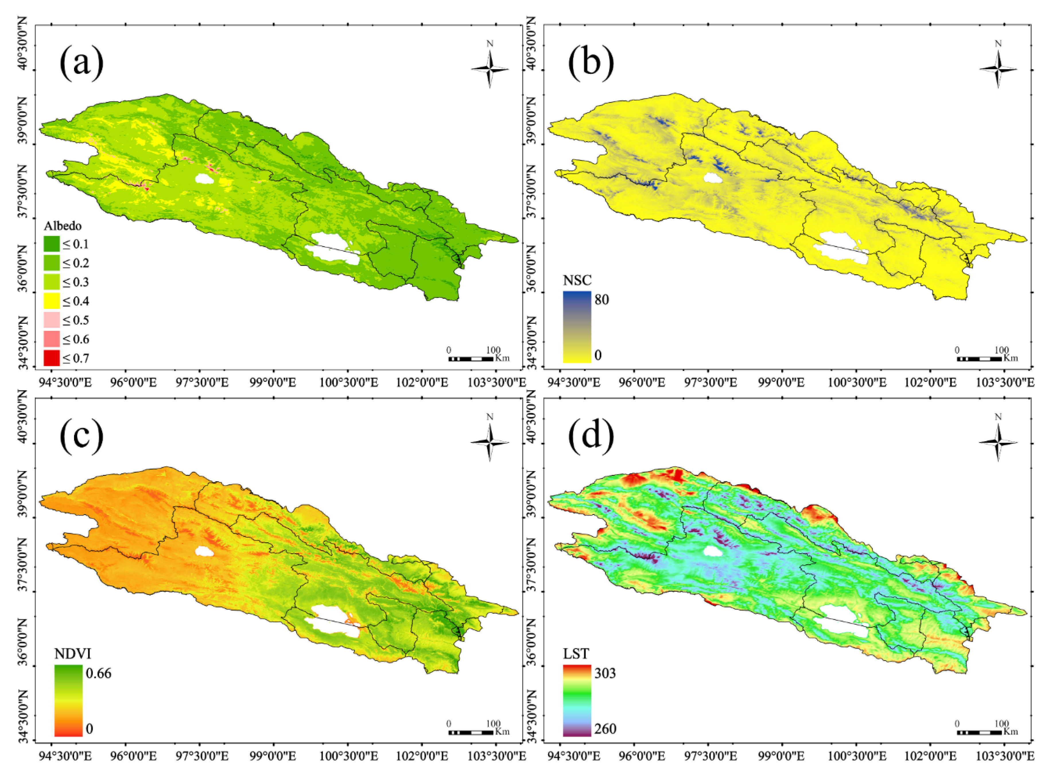
Figure 3. The multi-year average (a) albedo, (b) NSC, (c) NDVI, and (d) LST.
Atmosphere 15 01081 g003
Figure 4. Trends in the annual average albedo of the QLMs from 2001 to 2022 in relation to (a) annual average NSC, (b) annual average NDVI, (c) annual average LST; (d) trends in the average elevation and area percentage of PSI regions in the QLMs.
Atmosphere 15 01081 g004
Figure 5. The spatial distribution of significant or non-significant changes in (a) albedo, (b) NSC, (c) NDVI, and (d) LST in the QLMs from 2001 to 2022.
Atmosphere 15 01081 g005
Figure 6. Comparison of the multi-year monthly average values of albedo with (a) NSC, (b) NDVI, and (c) LST in the QLM region from 2001 to 2022.
Atmosphere 15 01081 g006
Figure 7. Monthly albedo anomalies (a) and monthly NSC anomalies, (b) and monthly NDVI anomalies, (c) and monthly LST anomalies in the QLMs from 2001 to 2022.
Atmosphere 15 01081 g007
Figure 8. (ae) Changes in explanatory power (q values) in 2001, 2006, 2011, 2016, and 2021.
Atmosphere 15 01081 g008
Figure 9. Striking differences in the driving factors (At a confidence level of 95%, “Y” indicates a significant difference in the spatial distribution of albedo due to the two factors, while “N” indicates the opposite).
Atmosphere 15 01081 g009
Figure 10. (ae) Changes in interactive explanatory power (q values) in 2001, 2006, 2011, 2016, and 2021; (f) average interactive explanatory power (q values) of 5 years (Bi: Enhance, bivariate, ENL: Enhance, nonlinear. The annotations inside parentheses indicate a higher frequency of occurrence of interaction types within five years. Without annotations, it indicates that the interaction types remained consistent over the 5 years).
Atmosphere 15 01081 g010
Table 1. IGBP land cover types.
IGBP Land Cover TypesAbbreviation
1 Evergreen Needleleaf ForestsENF
4 Deciduous Broadleaf ForestsDBF
5 Mixed ForestsMF
8 Woody SavannasWS
9 SavannasSav
10 GrasslandsGra
11 Permanent WetlandsPW
12 CroplandsCro
13 Urban and Built-up LandsUrb
15 Permanent Snow and IcePSI
16 Barrenbar
17 Water BodiesWB
The numbers represent the land cover types classified by IGBP within the QLMs region (arranged in ascending order).
Table 2. The datasets used in this study.
ParameterAbbreviationDatasetSpatial ResolutionTemporal ResolutionSource
AlbedoAlbedoMCD43A3500 mDailyhttps://lpdaac.usgs.gov (accessed on 1 May 2024)
Land Cover TypeLCTMCD12Q1500 mYearlyhttps://lpdaac.usgs.gov (accessed on 1 May 2024)
ElevationDemSRTM DEM30 m/https://cmr.earthdata.nasa.gov (accessed on 1 May 2024)
SlopeSlopeSRTM DEM30 m/
AspectAspectSRTM DEM30 m/
Land Surface TemperatureLSTMOD11A11000 mDailyhttps://lpdaac.usgs.gov (accessed on 1 May 2024)
Normalized Difference Vegetation IndexNDVIMOD13A1500 monce every 16 dayshttps://lpdaac.usgs.gov (accessed on 1 May 2024)
Normalized Difference Snow Index snow coverNSCMOD10A1500 mDailyhttps://nsidc.org (accessed on 1 May 2024)
Table 3. Types of interaction for two independent variables.
TypesInteraction TypesJudgment Criteria
Enhancetwo-factor enhancement q x 1 x 2 > M a x ( q x 1 , q x 2 )
Enhancenonlinear enhancement q x 1 x 2 > q x 1 + q x 2
Weakenone-factor nonlinear attenuation M i n ( q x 1 , q x 2 ) < q x 1 x 2 < M a x ( q x 1 , q x 2 )
Weakennon-linear attenuation q x 1 x 2 < M i n ( q x 1 , q x 2 )
Independentindependent q x 1 x 2 = q x 1 + q x 2
represents the interaction between two factors.
Disclaimer/Publisher’s Note: The statements, opinions and data contained in all publications are solely those of the individual author(s) and contributor(s) and not of MDPI and/or the editor(s). MDPI and/or the editor(s) disclaim responsibility for any injury to people or property resulting from any ideas, methods, instructions or products referred to in the content.