Abstract
Vehicle emissions belong to the category of near-surface sources, occur close to human activity areas, and pose a greater threat to human health than other anthropogenic pollution sources. Furthermore, the study of the spatiotemporal characteristics of near-road traffic pollution is of great significance to urban and regional ambient air quality management, and is also an important basis for vehicle emission inventories, as well as the assessment of ambient air impact. Most previous studies have analyzed the spatiotemporal characteristics of hydrocarbons (HCs), carbon monoxide (CO), nitrogen oxides (NOx), and carbon dioxide (CO2) in urban vehicle emissions over a certain time, without considering the synergistic effect of mobile source particulate matter, NOx, and volatile organic compounds (VOCs). In this study, we analyze the composition of vehicles with different emission standards from road mobile sources in Anqing City, China. National category III and IV vehicles are the main contribution sources of various pollutants, accounting for more than 60% of emissions. Although national category I and II vehicles accounted for less than 1% of the total number of vehicles, their contribution to emissions cannot be ignored, especially for CO and HCs, the contribution of which from such vehicles can reach about 7%. This is mainly due to the low level of pollution control arising from the larger emission factor and greater age of these vehicles. Furthermore, eliminating old cars and increasing the proportion of national category VI vehicles can effectively reduce vehicle pollutant emissions. In terms of the spatiotemporal distribution characteristics, highways around urban areas are also the main sources of heavy vehicles, and the emission intensity of these pollutants is also higher on national roads and highways surrounding urban areas. In addition, the presence of m/p-xylene and toluene solvent-using species is detected, which indicates that petrol vehicle emissions, LPG and petrol volatilization, and solvent-using sources contribute significantly to ozone formation in the ozone pollution process. Comparing weekdays and non-weekdays, the PM2.5 peaks on non-weekdays are significantly higher than those on weekdays, and there is no “weekend effect”, which indicates that traffic emissions have little influence on PM2.5 emissions, and may be related to energy use and industrial pollution. Overall, this study strengthens the understanding of the relationship between emissions, traffic volumes, and vehicle types on spatial and temporal scales, and emphasizes the need for further investigation and comprehensive measures to mitigate pollution from these emissions.
1. Introduction
As China’s urbanization accelerates and its economy grows, the number of motor vehicles and the accumulation of pollutants such as HC, CO, NOx, and CO2 in the atmosphere increase, particularly in urban areas. This contributes to significant impacts on ambient air quality, human health, and climate change [1]. Vehicle exhaust and evaporation emissions are important sources of near-surface ozone and secondary particle precursors in urban and regional areas. Based on PM2.5 source analysis results in recent years, motor vehicle pollution has gradually become the major source of haze pollution in many Chinese cities [2]. Moreover, vehicle emissions, as near-surface pollutants close to areas of human activity, present a more significant health risk than many other types of anthropogenic emissions [3]. Therefore, the study of vehicle pollutant emission characteristics and control measures is of great significance to urban and regional ambient air quality, and is also an important basis for the compilation of regional vehicle pollution emission inventories, the formulation of exhaust emission reduction measures, and the assessment of ambient air impact.
The investigation of spatial differences and temporal variation patterns is an important part of the research on vehicle emissions pollution [4]. The existing methods for vehicle emission inventory spatiotemporal analysis can be categorized as model-based [5,6,7,8,9,10] and data-driven methods [11,12,13,14,15,16,17,18]. For model-based methods, emission inventories are constructed based on macro traffic statistics such as vehicle ownership, fuel consumption, vehicle mileage, and average speed to calculate total emissions from mobile sources and predict future annual emission trends on a national or urban scale. The European Environment Agency (EEA) developed an inventory of road traffic emissions in the European Union from 1990 to 2013 [5]. The U.S. Environmental Protection Agency (EPA) establishes annual national emissions inventories based on state and local data [6]. Wu et al. [7] used the Mobile-China model to establish the MOBILE source emission inventory of Beijing from 1995 to 2009, and analyzed the emission reduction effect of emission control measures. Wang et al. [8] used the COPERT model to establish the interannual change in mobile source emissions in Beijing, Shanghai, Guangzhou, and other cities. Based on Vehicle Kilometers of Travel (VKT) and vehicle ownership statistics, Jin et al. [9] established a vehicle emission inventory for Liaoning Province from 2000 to 2016 with the COPERT model. Li [10] established emission factors of light vehicles and heavy diesel vehicles based on vehicle-mounted emission tests, and established domestic mobile source emission inventories combined with vehicle ownership and VKT. Emission inventories based on macro traffic statistics data require fewer model parameters, have a low calculation cost and easy implementation, and generate a regional static comprehensive emission total with low spatial and temporal resolution, which is suitable for the total emission accounting of cities, countries, and other large-scale regions.
Sensor-based data-driven methods, such as mobile plume chasing, on-board diagnostics (OBD), and remote sensing, have provided low-cost and highly efficient real-world measurements to complement regulated methods such as portable emission measurement systems (PEMS) tests and dynamometers [11,12]. Li et al. [13] proposed a vehicle driving conditions evaluation model that uses standardized mutual information to extract features with high NOx correlation from OBD real-time measurements. These advanced measurement tools generated abundant data and revealed new hot-spots that are often overlooked by regulated methods. Du et al. [14] deciphered the impact of urban traffic on air quality by combining multi-source real-time data such as traffic information, in situ surface-level pollutant concentrations, and meteorology. Liu et al. [15] developed a bottom-up method and established an on-road vehicle emission inventory of Foshan in 2014 with high spatiotemporal resolution on the basis of more detailed hourly traffic data covering all road types and regions. Ghaffarpasand et al. [16] used hour-by-hour traffic data and an IVE emission factor model to construct high-spatiotemporal-resolution emission inventories of different roads in large cities in Iran. Zhang et al. [17] established comprehensive emission profiles of organic compounds for typical Chinese diesel trucks. Wen et al. [18] developed updated vehicle emission inventories to make a comprehensive assessment of spatiotemporal variations and mitigation drivers of vehicle emissions in China from the past to the future. However, although there has been a lot of progress in the development of high resolution vehicle emission inventories, the spatiotemporal characteristics and sources of emissions in these cities suffer from a lack of attention.
Most previous studies have analyzed the spatiotemporal characteristics of HC, CO, NOx, and CO2 urban vehicle emissions over a certain time. As mobile source pollution has become an important source of air pollution as well as fine particulate matter in large and medium-sized cities in China, it is necessary to further analyze the synergistic effect of mobile source particulate matter, nitrogen oxide (NOx), and volatile organic compounds (VOCs). In this study, we firstly collected real-time observation data from traffic intersection monitoring stations and remote-sensing monitoring data, as well as vehicle inspection data, as detailed in Table 1. Then, we employed the International Vehicle Emission Model (IVE) and developed emission inventories based on vehicle ownership, average mileage, and unit energy consumption statistics. Finally, we analyzed the spatiotemporal distribution characteristics of near-road traffic pollution in Anqing City, China, and explored the proportions by source of VOCs, PM2.5, and NOx in depth. Overall, this study strengthens the understanding of the relationship between emissions, traffic volumes, and vehicle types on spatial and temporal scales, and emphasizes the need for further investigation and comprehensive measures to mitigate pollution arising from these emissions.

Table 1.
Data Sources.
2. Methodology
2.1. Study Area
There are 4 highways in Anqing, namely, Shanghai-Chongqing Expressway G50, Jinan-Guangzhou Expressway G35, Hefei-Anqing Expressway G4212, and Shanghai-Wuhan Expressway G42S, 3 national highways, namely, G105, G206, G318, and 7 provincial highways. The 3 national highways and the Hejiu Railway intersect in the city, and the city is connected to Chizhou City through the completed Anqing Yangtze River Highway Bridge and Anqing Yangtze River Railway Bridge and the under-construction Wangdong Yangtze River Bridge. Anqing represents a three-dimensional transportation network integrating highway, railroad, waterway, aviation, and oil and gas pipeline transportation, which indicates that the spatial and temporal distribution characteristics of traffic pollution in Anqing are worth studying. As shown in Figure 1, based on the regional distribution of Anqing City, Anhui River Avenue is selected as a typical road for traffic detection. This road is one of the important roads connecting the old city center and the development zone, and it is also one of the roads with large traffic flow in Anqing City. In addition, the Academy of Environmental Sciences is located on Wanjiang Avenue, one of the four major national control points in Anqing City, which can provide certain meteorological data and provide data support for traffic detection in Anqing City.
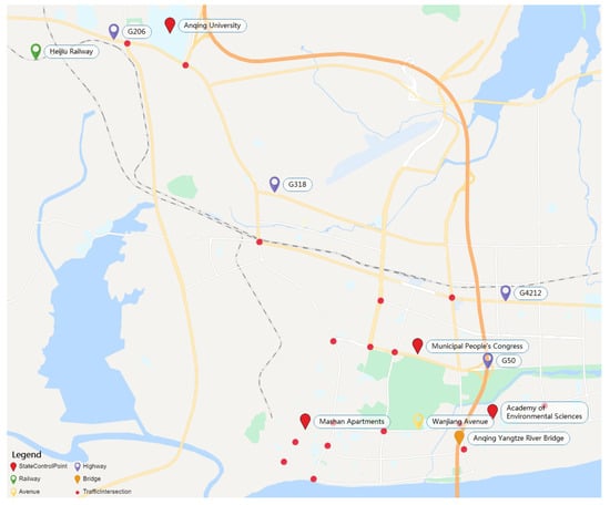
Figure 1.
The study area meets the needs of high traffic volume and multiple data collection sources. This map also illustrates the topography and related factors. The red dots indicate important traffic intersections and the triangles indicate the four state control points in Anqing.
The main data collected are shown in Table 1.
2.2. Emissions Characterization
The framework of the mobile source emission spatiotemporal inventory analysis is shown in Figure 2. We carried out a mobile and stationary VOCs and PM2.5 online source analysis and carbon emissions and NOx monitoring for no less than 14 days at different traffic hours (peak traffic periods (7:00–9:00 and 17:00–19:00), the off-peak period (9:00–17:00), and the low-peak period (22:00–6:00)) around the key traffic roads of the urban area of Anqing. PM2.5 online source analysis was carried out using single-particle aerosol mass spectrometry, VOCs online source analysis was carried out using mass spectrometry and gas chromatography/FID, and NOx monitoring was carried out using ionization chromatography and ionization mass spectrometry. The data were then cleaned to remove invalid and missing values. A database was set up to import, summarize, and organize the data, and filter useful information.
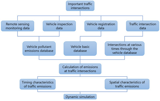
Figure 2.
Technical framework for mobile source investigations under typical scenarios.
Intersection passing data, vehicle information data, and remote-sensing monitoring point data were matched according to license plate number to obtain the intersection name, passing time, vehicle characteristics, and pollutant emission of each vehicle, and analyze the pollutant emission situation of major traffic intersections.
The collated pollutant emission data were also connected with the intersection coordinate vector data for dynamic visualization.
2.3. Selection of Test Methods for Discharged Pollutants
2.3.1. VOCs Measurements
Cruise monitoring cars were used for VOCs monitoring at different time periods to supplement the fixed-point detection to reduce the impact on the detection process of sources of pollution other than traffic. One of the cruise monitoring sections was the main Wanjiang Avenue, while the fixed-point detection location was on an auxiliary road of Wanjiang Avenue, at the Ecological Environment Bureau. Three periods of cruise monitoring were chosen, one each from the high-peak period (17:00–19:00), off-peak period (9:00–17:00), and low-peak period (22:00–24:00), with at least 1 h for collection and detection. Testing took place from 12 to 30 July 2022. The working principles of the collection equipment are detailed in [19,20]. The time-of-flight of each of the ions was recorded graphically by means of a data acquisition card, and the resulting data were processed to determine the components and content of the gas mixture.
2.3.2. PM2.5 and NOx Measurements
The process of PM2.5 measurement is divided into concentration determination and component detection [21]. Concentration determination was carried out using state-controlled point data of the Yingjiang District Ecological Environment Bureau, while component detection was accomplished using particulate matter collected at monitoring points during the corresponding time periods: peak (17:00–19:00), off-peak (9:00–17:00) and low (22:00–24:00). The collection particulate matter was tested in the laboratory for, among others, heavy metals and anionic components. Tests were carried out from 17 to 30 July 2022. Particulate matter was collected using a multi-channel constant-temperature and constant-flow atmospheric sampler with the parameters shown in Supplementary Materials Table S1.
Two main types of measurement methods were employed:
- Water-soluble anions in particulate matter in ambient air () were determined by ion chromatography (HJ 799-2016);
- Metal elements in particulate matter in air and exhaust gas were determined using inductively coupled plasma emission spectrometry (HJ 777-2015).
The testing instruments and reagents are shown in Supplementary Materials Table S2.
NOx measurements were made using automatic online monitoring [22].
2.4. Mobile Source Emission Inventory
2.4.1. Top-Down Methodology
A top-down approach was used to collect and investigate activity data such as motor vehicle ownership, emission factors, and average annual mileage to calculate the emissions of each pollutant from motor vehicles, as shown in Equation (1).
where is the emission of pollutant m, g; i is the serial number of the motor vehicle model; j is the serial number of the motor vehicle emission standard; is the number of motor vehicles of category i that meet the standard j, units; is the average annual mileage of motor vehicles of category i, km; and is the emission factor of pollutant m for motor vehicles of category i complying with standard j after localization correction, g/(km*vehicle).
2.4.2. Emission Factors
Based on the baseline emission factors of various types of motor vehicles in the Technical Guidelines for the Preparation of Air Pollutant Emission Inventories for Road Motor Vehicles, localized corrections were made by investigating the meteorology, motor vehicle driving conditions, etc., in Anqing City, and simulations were carried out. The calculation method is shown in Equation (2).
where is the composite baseline emission factor for pollutant m for class i motor vehicles complying with criterion j, g/(km-vehicle); is the environmental correction factor for class i motor vehicles; is the average speed correction factor for class i motor vehicles; is the deterioration correction factor for class i motor vehicles; and is the correction factor for other conditions of use of motor vehicles of category i, including sulfur content of oil and diesel vehicle load.
2.4.3. Localization Correction
The motor vehicle emission factor is affected by altitude, temperature, and humidity. Therefore, the meteorological correction factor consists of three parts, namely, a temperature correction factor, a humidity correction factor and an altitude correction factor, and the equation is as follows:
where is the temperature correction factor, is the humidity correction factor, and is the altitude correction factor. The temperature and humidity correction factors are generated by combining meteorological statistics for 2020, shown in Supplementary Materials Table S3, with the correction values contained in the “Technical Guidelines for the Preparation of the Inventory of Air Pollutant Emissions from Road Motor Vehicles”. The final temperature and humidity correction factors are shown in Table 2 and Table 3.
Table 2.
Temperature Correction Factor.
Table 3.
Humidity Correction Factor.
In terms of altitude correction, except for some mountainous areas in the Anqing region where the altitude exceeds 1500 m and the number of motorized vehicles is relatively small, the rest of the areas are within the range of 1000 and 1500 m. Under these conditions, an altitude correction is not required, in line with the guidance in the “Technical Guidelines for Preparation of Road Motor Vehicle Air Pollutant Emission Inventory”.
2.4.4. Determination of Correction Factor for Road and Traffic Conditions
The correction factor for road and traffic conditions is mainly based on the average local vehicle speed (km/h). The range of speeds is sub-divided into <20, 20–30, 30–40, and >40 km/h, and the 20–30 km/h range is corrected according to the local driving conditions, as shown in Table 4.
Table 4.
Motor Vehicle Average Speed Correction Factor.
2.4.5. Deterioration Correction
The deterioration correction factor uses 2014 as the base year, and the impact of mileage on pollutant emissions is projected based on the specific driving conditions of the vehicle, as shown in Table 5.
Table 5.
Motor Vehicle Emission Factor Degradation Factor.
2.4.6. Other Conditions
Other conditions-of-use corrections, as shown in Table 6, mainly consider the actual oil sulfur content, the ethanol blending degree of ethanol petrol, and the impact of diesel vehicle loading on motor vehicle pollutant emissions. In this study, we focus on the impact of oil sulfur content, with the ethanol blending degree of ethanol petrol and the impact of diesel vehicle loading not being considered as corrections, and the standard values in the Technical Guidelines for Preparation of Road Motor Vehicle Air Pollutant Emission Inventories are used.
Table 6.
Emissions Correction Factor for Sulfur Content of Motor Vehicle Oil.
Note that the correction items in Table 2, Table 3, Table 4, Table 5 and Table 6 are listed according to the actual type of vehicle, fuel type, emission standard, and oil product; the types not included are not listed in the table, and a value of 1.00 means that the item does not need to be corrected.
3. Experiment Results
3.1. Vehicle Inventory Analysis
Using the Mobile Source Emission Inventory methodology presented in Section 2.4, we can obtain the Anqing localization average annual pollutant emissions by vehicle, as shown in Supplementary Materials Tables S4 and S5.
In 2020, the total number of motor vehicles in Anqing City was 986,827, and the road mobile source CO, HC, and NOx, and total emissions of PM2.5 and PM10 were 2.65 × 10⁴ t, 2.94 × 10⁴ t, and 1.46 × 10⁴ t, and 2.13 × 10² t, and 2.32 × 10² t, respectively. The contribution to emissions of vehicles with different emission standards in Anqing City in 2020 is shown in Figure 3. National category III and IV vehicles are the main contribution sources of various pollutants, accounting for more than 60% of emissions, mainly because of the large number of national category III and IV vehicles—more than 70% of the total. Although the number of national category I and II vehicles accounted for less than 1% of the total, their contribution to emissions cannot be ignored, especially for CO and HC, where contributions from these vehicles reached about 7% of the total which is mainly due to the low level of pollution control arising from the larger emission factor and greater age of such vehicles. National category V vehicle ownership accounted for 20% of the total, but because of the high level of pollution control of vehicles of this type, especially in terms of the control of PM2.5 and PM10, the emissions are less. National category VI emission standards, implemented in China from July 2020, are more stringent than category V and pollutant emissions are lower. Thus, even though the proportion of national category VI vehicles is relatively low, their contribution to pollutants is even lower. By analyzing the composition of vehicles with different emission standards from road mobile sources in Anqing City, it can be seen that eliminating old cars and increasing the proportion of national category VI vehicles can effectively reduce vehicle pollutant emissions.
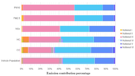
Figure 3.
Emission contribution of vehicles with different emission standards.
3.2. Spatial Distribution Characteristics
The numbers of vehicles passing through known intersections on non-working days and working days are shown in Supplementary Materials Figure S1. The intersection of North Linghu Road and North Huxin Road has the highest traffic volume, from which it can be concluded that this intersection has the highest vehicular pollutant emissions, while the intersection of Dekuan Road and Yanjiang Road has the lowest traffic volume, from which it can be concluded that this intersection has the lowest vehicular pollutant emissions. Furthermore, Supplementary Materials Figure S2 shows the specific visualization information based on two days of intersection traffic flow data from the traffic flow prediction and traffic flow data for visualization. The size of the traffic flow is indicated by the thickness of the flow line. This visualization shows that vehicles are mostly concentrated in Linghu South Road, Linghu North Road, Lake Road, Longmianshan Road, and Zhenfeng Avenue of the Linghu Scenic Area. Although the scenic area belongs to the downtown area of Anqing City, as a scenic area, it has fewer of the main vehicle types than other areas, and it can be seen that the serious pollution is concentrated around a few main roads in the Linghu Scenic Area.
3.3. Temporal Characteristics
For the time distribution characteristics analysis, the examined two days of intersection traffic data are divided into hourly data. The results are shown in Supplementary Materials Figure S3.
In terms of the weekday traffic flow, it can be seen that there are two peaks at 08:00 and 18:00, corresponding to people commuting to and from work, and at Midday, there is a small trough, corresponding to lunch break, On non-working days, the traffic flow is more moderate, with only one large peak at 18:00. In China, different number plate colors correspond to different vehicle types and ownership (private, commercial, official). Thus, we classified the number plates of the vehicles according to their colors and determined the proportion of each plate color. In order to represent this more intuitively, we turned the results into a pie chart, as shown in Figure 4a.
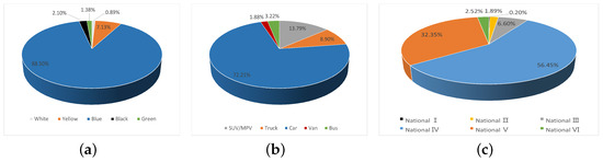
Figure 4.
Vehicle Classification Forecast. (a) Distribution of license plate types at important traffic intersections by percentage. (b) Distribution of vehicle types passing through important traffic intersections. (c) Distribution of vehicle emission standards of vehicles passing through important traffic intersections.
The proportion of vehicles with blue plates is the largest, reaching nearly 90%, while the proportion of vehicles with white plates is the smallest, less than 1%. This shows that the vehicles traveling in the urban area of Anqing are still dominated by blue-plate vehicles, so the main target should be these vehicles, and the aim should be to increase their emissions control. At the same time, the proportion of green-plate vehicles—corresponding to electric vehicles (EVs)—is only 1.38%, indicating that, currently, in Anqing, very few EVs are in use.
Next, we determined the proportions of different types of vehicles and the results are shown in Figure 4b. This shows that the vehicles traveling in the urban area of Anqing are mainly sedans, and thus, the main focus should be on sedans. Finally, we determined the proportion of vehicles classified according to the different types of emissions and the results are shown in Figure 4c. This shows that the emission types of most vehicles are categorized as National IV and National V, with National IV accounting for the largest proportion. This is related to the vehicle emissions policy promulgated by the national government. Most vehicles meeting only the National I, National II, and National III standards have already been phased out, so they account for a smaller proportion of the total. Similarly, the National VI standard has only just been implemented, so vehicles of this type also account for a small proportion of the total.
3.4. Spatiotemporal Distribution of Emissions at Important Traffic Intersections
The CO2, CO, NO and HC emissions of the 11 intersections under investigation were analysed and processed. The intersection passing data, vehicle information, and remote-sensing monitoring point data were matched to vehicle license plate number to obtain the passing time, vehicle information, and pollutant emissions of each vehicle passing through the intersection. The results of this analysis are shown in Supplementary Materials Figure S4.
Traffic flow data showed that the intersection of North Linghu Road and North Huxin Road has the highest traffic flow, so the vehicle pollutant emission at this intersection were expected to be the highest, while the intersection of Dekuan Road and Yanjiang Road has the lowest traffic flow, so the vehicle pollutant emissions at this intersection were expected to be the lowest. It can be seen that the pollutant emissions are basically consistent with the changes in traffic flow.
The four kinds of pollutants were analyzed in terms of the color of the license plates of the vehicles contributing to their emission. As vehicles with green license plates (EVs) do not emit pollutants, only the statistics for vehicles with blue and yellow license plates are shown in the pie chart in Supplementary Materials Figure S5. It can be seen that the proportion of pollutants emitted by the vehicles with blue license plates is the largest, which is due to most vehicles falling into this category.
Figure 5 shows the proportion of emissions contributed by vehicles passing through the intersections categorized according to emission standards. It can be seen that emissions from National IV and National V standards vehicles account for 90% of the total, for the same reasons as discussed above.
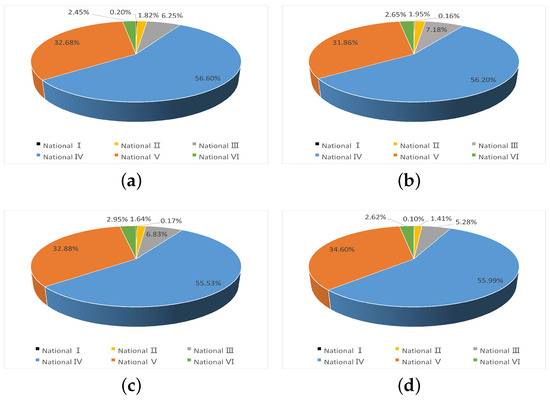
Figure 5.
Distribution of Different Emissions from Passing Vehicles at Intersections. (a) Distribution of CO2 Emissions from Passing Vehicles at Intersections. (b) Distribution of CO Emissions from Passing Vehicles at Intersections. (c) Distribution of NO Emissions from Passing Vehicles at Intersections. (d) Distribution of HC Emissions from Passing Vehicles at Intersections.
Pavement monitoring data, including NO2, O3, PM2.5, PM10, and TVOC data provided by the Anqing Environmental Monitoring Station were visualized and analyzed, and the specific visualization results are shown in Supplementary Materials Figure S6.
The spatial distribution of pollutants in Anqing shows that the spatial distribution of pollutant emissions from motor vehicles is basically the same as the distribution of the road network, and that the pollutant emissions from motor vehicles are distributed along highways and other roads in a band-like manner. TVOC emissions are mainly concentrated in the Xicheng District, the eastern part of the new city, and the non-city area; this is due to the above pollutants mainly arising from light buses, and the traffic flow of light buses in the western part of the city is larger, the eastern part of the new city, and the non-city area. For the pollutants NO2, PM2.5, and PM10, urban areas are the main source. Heavy trucks are also a major source of such pollutants. Thus, emissions of these pollutants are also higher on highways around the urban areas, where most heavy vehicles are found.
At the same time, emissions from National IV and National V standards motor vehicles at important traffic intersections in Anqing accounts for 90% of the total. Similarly, the proportion of vehicles meeting the newly released National VI standard is very small and does not even exceed the proportion of National III standard vehicles, which makes Anqing’s emissions higher.
3.5. VOCs Distribution Analysis
3.5.1. VOCs Concentration
From 12 to 30 July 2022, the total concentrations of 50 VOCs (denoted as ∑VOCs, actually only 46 VOCs were detected) at the Anqing Ecological and Environmental Protection Bureau site ranged from 30.75 to 214.45 ppbv, with an arithmetic mean of 67.21 ppbv, a median of 54.16 ppbv, and a geometric mean of 51.76 ppbv. The trend in the hourly values of VOCs automatically detected by the Ecological Environment Bureau from 12 July to 17 July 2022 is shown in Figure 6. As can be seen, the overall trend in VOCs first increases then decreases and then increases again. From 0:00 to 6:00, the concentration of VOCs increased, from 6:00 to 18:00, the concentration of VOCs decreased, and from 18:00 to 24:00, the concentration of VOCs increased. This is mainly related to two factors. Firstly, during the daytime, the atmospheric temperature is high, solar radiation is strong, and thus, the photochemical reaction of VOCs is strong. Thus, with the prolongation of time, the concentration of VOCs shows a decreasing trend. However, after 18:00, the intensity of solar radiation decreases, the intensity of photochemical reaction becomes weaker, and the concentration of VOCs rises. Secondly, it is possible that there is an increase in the number of large vehicles during the night, which to a certain degree increases the concentration of VOCs during the night. Comparing the concentration trends on weekdays and non-workdays, the “weekend effect” of VOCs is more obvious, in the range of 0:00 to 12:00, the concentration of VOCs on weekdays is much higher than that on non-workdays, which is mainly related to the use of motor vehicles. As shown in Supplementary Materials Figure S7, the concentration of five categories of VOCs, namely, alkanes, olefins, aromatic hydrocarbons, halogenated hydrocarbons, and oxygenated sulfur compounds, decreased significantly in the afternoon. This is mainly due to the high temperatures in the afternoon, resulting in obvious photochemical reactions and secondary production of O3. However, alkanes, halogenated hydrocarbons, and oxygenated sulfur compounds all started to increase again at 20:00 and peaked at 4:00–5:00, before gradually decreasing again with a trough in the afternoon. On the one hand, the temperature drops at night and the atmospheric boundary layer is lowered, which leads to an increase in concentration, and on the other hand, it cannot be ruled out that some enterprises may have production emissions at night. Although olefins and aromatic hydrocarbons showed a clear trough in the afternoon, they gradually increased during the night and peaked at 8:00.
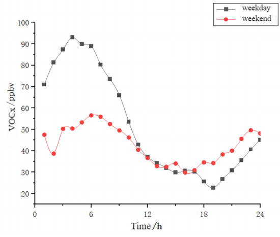
Figure 6.
Hourly Variation in VOCs Concentration.
3.5.2. VOCs Components Characterization
A total of 50 volatile organic compounds (VOCs), including alkanes, olefins, aromatic hydrocarbons, halogenated hydrocarbons, and organic compounds containing oxygen, nitrogen and sulfur, were searched for. Dimethylformamide, ethyl formate, carbon disulfide (propyl mercaptan), and n-decanol were not detected, giving a total of 46 substances detected. Of these 46 substances, 15 were detected with similar results, with little variation over time. The specific results are shown in Supplementary Materials Table S6. There were also eight substances that did not conform to the overall pattern of change, changing only 1–2 times during the measurement process and remaining within a certain range for the rest of the time period, with the specific concentrations shown in Supplementary Materials Table S7.
Nonane, dimethylbenzene (ethylbenzene), trimethylbenzene, trichloroethylbenzene, and diethylbenzene showed peaks on 20 July, while toluene peaked on 25 July and dimethylbenzene (ethylbenzene) peaked again on 30 July. The coefficients of variation (CV) were 2.09, 1.97, 1.89, 1.62, 0.82, and 0.76, respectively. All of the above peaks were well above the mean, and the average values of the substances were higher than the average values at the peak of 20 and the low of 30 July. The concentrations of xylene (ethylbenzene) measured during the peak period on 20 July and the low peak period on 30 July accounted for 37% and 52% of the total emissions, respectively, and it was initially concluded that there was a sudden event that caused the concentration of VOCs to spike. Meanwhile, it was found (as shown in Supplementary Materials Figure S8) that the concentration of VOCs in the ambient air of Anqing City was composed of methylene chloride, which accounted for about 23.1% of the volume percentage of TVOCs, followed by n-hexane, which accounted for 13.3% of the overall TVOCs. Iso-pentane and chloromethane accounted for 3.3% and 2.2% of the TVOCs, respectively, and the other VOCs accounted for a total of 58.9%.
3.5.3. VOCs Source Analysis
The isopentane/n-pentane ratio is often used to characterize emissions from combustion sources. An isopentane/n-pentane ratio of about 2.93 is indicative of motor vehicle emissions, coal combustion ratios range from 0.56 to 0.80, and liquid gasoline and fuel evaporation ratios range from 1.50 to 3.00 and 1.80 to 4.60, respectively. As shown in Figure 7a, the isopentane/n-pentane ratios in this study ranged from 1.82 to 5.07, with a mean value of 3.27 ± 0.68, indicating that gasoline combustion evaporation dominates. Meanwhile, isopentane/n-pentane showed a significant exponential relationship, indicating that they come from the same source.
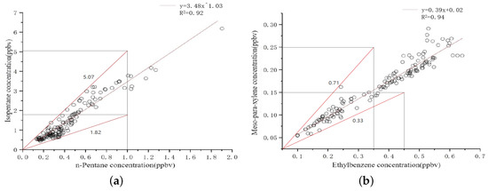
Figure 7.
R2 analysis of (a) Isopentane/n-Pentane and (b) Meso-para-xylene/Ethylbenzene at the Anqing ECO site.
The benzene/toluene ratio is widely used for the initial determination of the source of a pollutant. Benzene is a typical species of mobile source VOCs, and toluene is affected by a variety of sources including mobile sources, organic solvent volatilization sources and combustion sources. The benzene/toluene (B/T) ratio is usually used to study motorized and non-motorized sources, and B/T = 0.5 is used as an approximation of the source of VOCs from motorized vehicles; when B/T > 1, it indicates a strong combustion source in the vicinity, while when B/T is much less than 0.5, it is less affected by mobile sources and more related to organic solvent (toluene source). As shown in Figure 7b, the benzene/toluene ratios in this study ranged from 0.29 to 2.82, reflecting mixed pollution of the local ambient air, with a mean value of 1.00 ± 0.49, indicating a larger proportion of the combined effects of mainly motorized mobile sources, bio-fuels, and coal-consuming processes, and a smaller proportion of the effects of industrial pollution.
The photochemical reaction activity of p/m-xylene is higher and its residence time in the atmosphere is shorter than that of ethylbenzene, and the active species are constantly consumed in the photochemical reaction. Thus, the ratio of p/m-xylene to ethylbenzene (X/E) can be used to evaluate the degree of aging of the air mass. As shown in Figure 7b, the ratios of p/ m-xylene/ethylbenzene in this study ranged from 0.33 to 0.71, with a mean value of 0.35 ± 0.06. The X/E ratios in this study are lower than those of other studies (1.42–2.95), indicating that aging of the air mass at the ambient air station in Anqing City exists, which is affected by the sampling time, the photochemical activity of the atmosphere, and the transmission distance, etc. Meanwhile, the linear correlation between ethylbenzene and m-para-xylene is obvious, indicating that these two compounds come from the same source.
3.5.4. VOCs Ozone Potential Analysis
The ozone production potential (OFP) reflects the relative contribution of each type of VOC to ozone production and is an important parameter to measure the reactivity of VOC species [23,24,25,26,27]. In this study, the ozone production potential (OFP) was calculated based on the corrected value of max incremental reactivities (MIR) given by the latest data from California administrative code, dating from 2010 [28], and the calculation formula was as follows:
where is the ozone production coefficient (g × g−1) for a particular VOC compound in the ozone maximum increment response, and the coefficients in this study are quoted from the most recent data from the California administrative code (2010). is the actual observed ambient concentration of a particular VOC in ppbv. The coefficients are shown in Table 7.
Table 7.
MIR Values for Different Species.
As shown in Figure 8, during the automatic monitoring period from 12 to 17 July, the variation in OFP ranged from 17.1 to 101.6 ppbv, with an arithmetic mean of 59.8 ± 17.1 ppbv, to which alkanes contributed 34.00%, alkynes 47.58%, and benzenes 18.41%. It can be seen that alkyne hydrocarbons have lower concentrations but contribute the most to ozone generation, followed by alkanes, with benzene contributing the least to ozone. The mean OFP of n-hexane was 11.324 ± 9.974 ppbv, which contributed 18.93% and was the highest contributor to the emissions, followed by isoprene and ethylene with 10.82% and 8.85%, respectively. Of the top-ten species, 1-pentene, ethylene, and propylene are related to vehicle emissions, while cyclohexane and isopentane are related to LPG and petrol volatilization. In addition to this, m/p-xylene and toluene are the identified solvent-using species, which can indicate that petrol vehicle emissions, LPG and petrol volatilization, and solvent-using sources contribute significantly to ozone formation in the ozone pollution process. Therefore, the control of these pollutants needs to be strengthened.
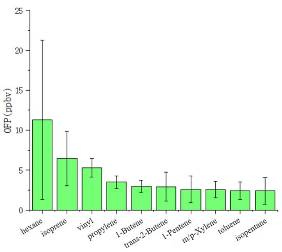
Figure 8.
Top 10 compounds contributing to the ozone potential of the Anqing ambient air site.
3.6. PM2.5 Distribution Analysis
3.6.1. Concentration Distribution Characteristics of PM2.5
The trend in hourly values of PM2.5 is shown in Figure 11a. Across the day, the concentration of PM2.5 first increases and then decreases. From 02:00 to 12:00, the PM2.5 concentration shows an increasing trend, and the concentration is highest at 10:00–11:00. From 12:00 to 02:00 the next day, the concentration shows a decreasing trend, and the concentration is lowest at 01:00–02:00. This is mainly related to atmospheric activity; during the daytime, when the temperature is high and atmospheric stability is high, the particulate matter cannot easily diffuse, and the concentration is increased; then, when the temperature decreases, the wind increases, and atmospheric activity becomes strong and it become easy for particulate matter to diffuse, and thus, the concentration of particulate matter decreases. Furthermore, there is no obvious peak during the morning and evening peak traffic flow periods, indicating that the morning and evening peaks are not obvious at this location. Comparing the difference between weekdays and non-weekdays, the PM2.5 peaks on non-weekdays are significantly higher than those on weekdays, and there is no “weekend effect”, which indicates that traffic emissions have little influence on PM2.5 emissions, and may instead be related to energy use and industrial pollution.
3.6.2. Characterization of PM2.5 Components
As shown in Figure 9, the atmospheric particulate matter in Anqing is dominated by ions, with a mean value of 147 ± 54.9 μg/m3, followed by with a concentration of 7.3 ± 3.9 μg/m3, with a content of 6.7 ± 3.1 μg/m3, and with a concentration of 3.7 ± 5.1 μg/m3, whereas , , and were not detected. The overall water-soluble anion content ranged from 56.2 to 301 μg/m3, with a mean concentration of 168 ± 56 μg/m3.
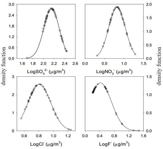
Figure 9.
Concentration distribution of four anions in atmospheric particulate matter in Anqing city.
In order to recognise the enrichment status of these elements in particulate matter, enrichment factors are used in this project, which are calculated as follows:
where is the enrichment factor of element i in atmospheric particulate matter, and are the concentrations of elements i and in atmospheric particulate matter, and and are the abundances of elements i and in crustal surface soils, respectively [29,30,31,32].
Based on this calculation, the enrichment of each element is shown in the Figure 10. The average EF value of 17 elements is greater than 1, which reflects the enrichment of these elements in the atmospheric particulate matter, and the average EF value of Mn, V, and Co is less than 1.0, which, on the one hand, indicates that the large surface area of the atmospheric PM2.5 can easily enrich heavy metal elements, and on the other hand, it can also reflect the source of these elements. The EF value of Zn is the highest, with the average value of 1090 ± 220; the average EF value of Cd is 136 ± 142; the average EF value of As is 118 ± 43; the average EF value of Mo is 111 ± 64; the average EF value of Bi is 111 ± 64; the average EF value of Bi is 111 ± 64.220; the average value of EF for Cd is 136 ± 142; the average value of EF for As is 118 ± 43; the average value of EF for Mo is 111 ± 64; and the average value of EF for Bi is 112 ± 111. The enrichment of these elements in the atmospheric particulate matter of Anqing was very obvious. Zn, Cd, As, and Mo were highly enriched; Ba, Ag, Cr, Be, Pb, Sr, Sb, Cu and Sn were moderately enriched, with EFs between 10 and 100; and Ni, Li and U were mildly enriched with EFs lower than 10 but greater than 1. However, V, Co, and Mn had EFs of less than 1.0 in atmospheric particulate matter, reflecting a deficit state. In addition, the EF values of Cd, Cr, Mo, Bi, Ag, Sb, and Ni were highly variable, with standard deviations greater than 50%, which indicated a large variability in the enrichment of these elements during the sampling period, further reflecting that they may have different sources in different sampling periods. The small variations in the enrichment of Zn, As, and Ba in these samples indicate that these elements are stable in the particulate matter and their sources are fixed.
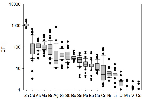
Figure 10.
Enrichment characteristics of different elements in atmospheric particulate matter in Anqing.
3.7. NOx Distribution Analysis
The trend in hourly values of NOx is shown in Figure 11b. Across the day, NOx values show a trend of increasing then decreasing and then increasing again. From 0:00 to 7:00, the values show an increasing trend, from 7:00 to 16:00, a decreasing trend with the lowest concentration being at 14:00; and then, from 16:00 to 24:00, the trend increases again with the highest concentration at 23:00. This is mainly related to the photochemical reaction of NOx. From 7:00 onward, the temperature rises, the intensity of solar radiation is high, and the photochemical reaction is strong, which leads to the photolysis of NO2 and a decrease in NOx concentration. At the same time, the temperature is highest at 14:00–15:00, and thus, at this time, the intensity of photochemical reactions is the highest, and the concentration of NOx is the lowest; after 16:00, the intensity of solar radiation is low, and the intensity of photochemical reactions is lowered, and the concentration of NOx increases. NOx concentrations show a clear “weekend effect”, with weekday NOx concentrations generally higher than non-weekday concentrations, which is mainly related to the heavy use of motor vehicles on weekdays and the consequent traffic congestion.
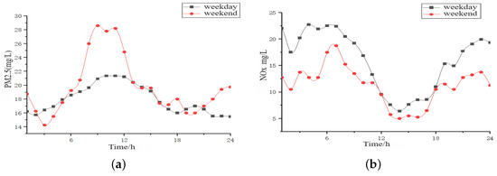
Figure 11.
Hourly variation in (a) PM2.5 and (b) NOx.
Generally speaking, NO2 is mainly emitted from mobile sources, while SO2 is mainly emitted from stationary sources. Meanwhile, CO is produced during incomplete combustion of fuels, especially during combustion with insufficient air, as in such situation, only a small amount of CO can be converted to CO2, and a large amount of CO will remain in the flue gas. Therefore, the ratio of NO2/SO2 and CO/NO2 can be used to determine whether NO2 and SO2 in the ambient air originate from coal combustion emissions. As shown in Figure 12a, the ratio of NO2/SO2 for emissions from coal combustion as the main process is generally below 1.0, while those above 1.0 are considered to be mobile sources. The ratio of NO2/SO2 in the ambient air of Anqing City is 2.68, much higher than the ratios in the industrial area and the urban area, reflecting the pollution characteristics of motor vehicle emissions. The daily change pattern of NO2/SO2 shows that the ratio decreases significantly in the afternoon, reflecting the obvious transformation process of NO2.
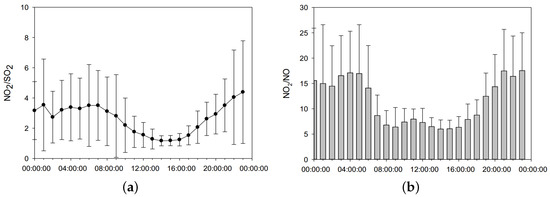
Figure 12.
Daily Patterns of (a) NO2/SO2 and (b) NO2/NO.
At the same time, NO2 can absorb energy to produce NO and O under light conditions, and then combine with O2 to produce O3, while O3 can react with NO to produce NO2 and O2. Therefore, the NO2/NO ratio can reflect the efficiency of the photochemical reaction, and further reflect the strength of the atmospheric oxidative capacity, which is one of the indicators of the formation of the photochemical secondary pollutant O3 [33]. The ratio of NO2/NO in the ambient air of Anqing City is 11.5, especially at night (Figure 12b), and the ambient air has a very strong ability to generate O3.
4. Discussion
During the study period, the areas with high emission pollution and high traffic flow were concentrated around important traffic intersections, and the spatial distribution of motor vehicle pollutant emissions was basically consistent with the distribution of the road network, with motor vehicle pollutant emissions showing a banded distribution characteristic along motorways and other highways. This spatial pattern is consistent with previous in situ investigations of emission characteristics [34]. Due to long-term industrial development and urbanization, Anqing has become an area of high background emission concentration and serious pollution in Anhui Province. The spatial aggregation of dense population can be mainly attributed to the economic and industrial growth of the city, which has resulted in high traffic flow in the city center area of Anqing. As a result, the Anqing city center area is exposed to a greater risk of pollution due to the consistent spatial distribution of emissions pollution and population density.
From the traffic flow, it can be seen that on weekdays, the two peaks of traffic flow occur at 08:00 and 18:00, corresponding to people commuting to and from work, and there is a small trough at Midday, corresponding to lunch break; whereas the traffic flow on non-weekdays is more moderate, with no major peaks during the day, and only a small peak at 18:00. The trend is very similar between weekdays and non-weekdays. The trend in traffic flow curves on weekdays and non-weekdays is very similar, and the traffic flow at important intersections does not change significantly depending on whether it is a working day or not. At the same time, from the statistics of the distribution of license-plate colors at important intersections, it can be seen that the vehicles passing by these important intersections are mainly blue-plate National IV and National V cars. Combined with the distribution of pollutant emissions at the intersections, it can be seen that the main source of pollutants is precisely these blue-plate cars, and although the emissions of National I, II, and III vehicles are very serious, the number of these vehicles is small, which results in their emissions accounting for a relatively small proportion of the total emissions. The proportion of emissions from National IV vehicles is almost double that of National V vehicles, which is in line with the results of the intersection crossing survey, where the proportion of National IV vehicles is the same as that of National V vehicles, and the distribution of the two is highly consistent.
From the results of pollutant analysis, the “weekend effect” of VOCs and NOx is more obvious. From 0:00 to 12:00, the concentration of VOCs on weekdays is much higher than that on non-weekdays. Meanwhile, the concentration of NOx on weekdays is generally higher than that on non-weekdays, which is mainly related to the large number of motor vehicles in use on weekdays, as well as the subsequent traffic congestion. In the source analysis of VOCs, the ratio of isopentane/n-pentane ranged from 1.820 to 5.070, with a mean value of 3.278 ± 0.688, indicating that gasoline combustion and evaporation were dominant. The obvious exponential relationship between isopentane/n-pentane indicated that they came from the same source. The ratio of benzene/toluene ranged from 0.29 to 2.82, indicating that the local ambient air was polluted by a mixture of pollution types, and the mean value was 1.00 ± 0.49, indicating that it is mainly affected by motor vehicle mobile sources, bio-fuels, and coal consumption process together in a larger proportion, and less by industrial pollution. In the source analysis of NOx, the ratio of NO2/SO2 in the ambient air of Anqing City is 2.68, much higher than the ratios of industrial and urban areas, indicating that motor vehicle tailpipe emissions are the main source of this type of pollution.
However, when comparing weekday and non-weekday PM2.5 analyses, the PM2.5 peaks on non-weekdays are significantly higher than those on weekdays, and there is no weekend effect, suggesting that traffic emissions do not have a significant impact on PM2.5 emissions, which may be related to energy use and industrial pollution. Meanwhile, Zn, As, and Ba in the PM2.5 samples have small differences in enrichment, indicating that these elements are more stable and come from a fixed source in the particulate matter. Zn is the most common catalyst for hydrogenation, so the enrichment of Zn in the atmospheric particulate matter may originate from the use of the catalyst. In addition, ZnO is often used as a desulfurizing agent, commonly used for desulfurization of high-sulfur materials in industrial processes. Considering the actual development process of the regional city and industry, and the high concentration in the atmospheric particulate matter, the Zn in the atmospheric particulate matter originates from historical use, and then enters the atmosphere in the form of dust following the later demolition or reconstruction of the plant. The main sources of PM2.5 in Anqing are energy use and industrial pollution.
In addition, the main pollutants from mobile sources, VOCs and NOx, have a huge impact on O3 production. The ozone generation potential was calculated in the collected VOCs samples. Of the top-10 species, 1-pentene, ethylene, and propylene were associated with vehicle emissions, and cyclohexane and isopentane were associated with LPG and petrol volatilization. In addition, m/p-xylene, and toluene were the identified solvent-using species, which indicates that petrol vehicle emissions, LPG and petrol volatilization, and solvent-using sources make a significant contribution to ozone formation during the ozone pollution process. The contribution of gasoline vehicle emissions, LPG and gasoline volatilization, and solvent use sources in ozone pollution processes is important for ozone formation.
At the same time, NO2 can absorb energy to produce NO and O under light conditions, and then combine with O2 to produce O3. Conversely, O3 can react with NO to produce NO2 and O2, so the NO2/NO ratio can reflect the efficiency of the photochemical reaction, and further reflect the strength of the atmospheric oxidation capacity, which is one of the indicators of the formation of photochemical secondary pollutants O3. The ratio of NO2/NO in the ambient air of Anqing is 11.5, especially at night, and the ambient air has a very strong ability to generate O3. Therefore, there is a need to strengthen the control of VOCs and NOx.
5. Conclusions
Based on the traffic flow data of 17 important traffic intersections in Anqing, vehicle registration data, and remote-sensing monitoring data at environmental monitoring stations, this study analyzes the spatiotemporal distribution characteristics of near-road traffic pollution in Anqing. The areas with high emission pollution and high traffic flow are concentrated around important traffic intersections, the spatial distribution of vehicle emissions is basically the same as the distribution of the road network. Furthermore, the vehicle emissions show a banded distribution characteristic along the highways and other highways, while the traffic flow in Anqing on weekdays versus non-weekdays is not very influential. In addition, the main pollutants emitted by mobile sources in Anqing are VOCs and NOx, which contribute greatly to the increase in O3 content in the atmosphere, and thus, require more control. Overall, this study strengthens the understanding of the relationship between emissions, traffic volumes, and vehicle types on spatial and temporal scales, and emphasizes the need for further investigation and comprehensive measures to mitigate pollution from these emissions.
Supplementary Materials
The following are available at https://www.mdpi.com/article/10.3390/atmos15040417/s1, Table S1: Atmospheric Sampler Parameters, Table S2: Testing Instruments and Reagents, Table S3: Meteorological Statistics of Anqing City, 2020, Table S4: Average annual pollutant emissions per vehicle (Gasoline), Table S5: Average annual pollutant emissions per vehicle (Diesel), Table S6: Concentrations of 15 Substances with Insignificant Changes, Table S7: Concentration of 8 Substances, Figure S1: Distribution of traffic flow at different traffic intersections, Figure S2: Visualization of weekday and non-weekday traffic data, Figure S3: Characteristics of the temporal distribution of traffic flow data, Figure S4: Characterization of the distribution of pollutant emissions from passing vehicles at intersections, Figure S5: Distribution of Different Emissions, Figure S6: Visualization of Emissions, Figure S7: Daily trends in different types of VOCs, Figure S8: Major VOCs percentage of TVOCs.
Author Contributions
Conceptualization, B.L. and J.L. (Jiaren Li); methodology, B.L. and Z.X.; software, B.L. and J.L. (Jiaren Li); validation, J.L. (Jiang Lu) and Z.X.; formal analysis, J.L. (Jiang Lu); investigation, B.L.; resources, J.L. (Jiang Lu) and Z.X.; data curation, J.L. (Jiaren Li); writing—original draft preparation, B.L. and J.L. (Jiaren Li); writing—review and editing, Z.X.; visualization, J.L. (Jiaren Li) and J.L. (Jiang Lu); supervision, Z.X.; project administration, Z.X.; funding acquisition, Z.X. All authors have read and agreed to the published version of the manuscript.
Funding
This work was supported in part by the National Natural Science Foundation of China (62033012, 62103124), the Major Special Science and Technology Project of Anhui (202003a07020009, 201903a07020012), and the Open Project Program of Anhui Provincial Key Laboratory of Multimodal Cognitive Computation (Anhui University) under grant MMC202303.
Institutional Review Board Statement
Not applicable.
Informed Consent Statement
Not applicable.
Data Availability Statement
The data presented in this study are available on request from the corresponding author. The data are not publicly available due to privacy.
Conflicts of Interest
Jiang Lu is employees of Hefei Branch of China Telecom Co., Ltd. The company had no roles in the design of the study; in the collection, analysis, or interpretation of data; in the writing of the manuscript, or in the decision to publish the articles. The paper reflects the views of the scientists and not the company. The authors declare no conflicts of interest.
References
- Lu, P.; Tuheti, A.; Deng, S.; Li, G.; Liu, J. Spatial Distribution and Inter-City Transport of PM2.5 Concentrations from Vehicles in the Guanzhong Plain in Winter. Atmosphere 2023, 14, 1748. [Google Scholar] [CrossRef]
- Xing, Q.; Sun, M. Characteristics of PM2.5 and PM10 Spatio-Temporal Distribution and Influencing Meteorological Conditions in Beijing. Atmosphere 2022, 13, 1120. [Google Scholar] [CrossRef]
- Ghorani-Azam, A.; Riahi-Zanjani, B.; Balali-Mood, M. Effects of air pollution on human health and practical measures for prevention in Iran. J. Res. Med Sci. Off. J. Isfahan Univ. Med Sci. 2016, 21, 65. [Google Scholar]
- Xu, Z.; Kang, Y.; Cao, Y.; Li, Z. Spatiotemporal Graph Convolution Multifusion Network for Urban Vehicle Emission Prediction. IEEE Trans. Neural Netw. Learn. Syst. 2021, 32, 3342–3354. [Google Scholar] [CrossRef] [PubMed]
- Agency, E.E. European Union emission inventory report 1990–2013 under the UNECE Convention on Long-range Transboundary Air Pollution (LRTAP). Akusherstvo I Ginekol. 2010, 42, 22–33. [Google Scholar]
- Zhang, Y.; Wang, W.; Wu, S.Y.; Wang, K.; Minoura, H.; Wang, Z. Impacts of updated emission inventories on source apportionment of fine particle and ozone over the southeastern U.S. Atmos. Environ. 2014, 88, 133–154. [Google Scholar] [CrossRef]
- Ye, W.U.; Wang, R.; Zhou, Y.U.; Lin, B.; Lixin, F.U.; Kebin, H.E.; Hao, I. On-road vehicle emission control in Beijing: Past, present, and future. Environ. Sci. Technol. 2011, 45, 147. [Google Scholar]
- Wang, H.; Fu, L.; Zhou, Y.; Du, X.; Ge, W. Trends in vehicular emissions in China’s mega cities from 1995 to 2005. Environ. Pollut. 2010, 158, 394–400. [Google Scholar] [CrossRef] [PubMed]
- Jin, J.; Sun, S.; Wang, F.; Ling, Y.; Wang, T.; Wu, L.; Wei, N.; Chang, J.; Mao, H. Vehicle Emission Inventory and Scenario Analysis in Liaoning from 2000 to 2020. Environ. Sci. 2020, 41, 665–673. [Google Scholar]
- Li, M. Research on Mobile Pollution Source Emission Inventories. Ph.D. Thesis, Beijing Institute of Technology, Beijing, China, 2016. [Google Scholar]
- Wang, H.; Wu, Y.; Zhang, K.M.; Zhang, S.; Baldauf, R.W.; Snow, R.; Deshmukh, P.; Zheng, X.; He, L.; Hao, J. Evaluating mobile monitoring of on-road emission factors by comparing concurrent PEMS measurements. Sci. Total Environ. 2020, 736, 139507. [Google Scholar] [CrossRef]
- Zhang, S.; Zhao, P.; He, L.; Yang, Y.; Liu, B.; He, W.; Cheng, Y.; Liu, Y.; Liu, S.; Hu, Q.; et al. On-board monitoring (OBM) for heavy-duty vehicle emissions in China: Regulations, early-stage evaluation and policy recommendations. Sci. Total Environ. 2020, 731, 139045. [Google Scholar] [CrossRef] [PubMed]
- Li, J.; Xu, Z.; Cao, Y.; Xia, X.; Kang, Y. Emission Evaluation for Diesel Vehicles Under Typical Operating Conditions. In Proceedings of the 2023 International Conference on Advanced Robotics and Mechatronics (ICARM), Macau, China, 8–10 July 2023; pp. 686–690. [Google Scholar]
- Du, W.; Chen, L.; Wang, H.; Shan, Z.; Zhou, Z.; Li, W.; Wang, Y. Deciphering urban traffic impacts on air quality by deep learning and emission inventory. J. Environ. Sci. 2023, 124, 745–757. [Google Scholar] [CrossRef] [PubMed]
- Liu, Y.H.; Ma, J.L.; Li, L.; Lin, X.F.; Xu, W.J.; Ding, H. A high temporal-spatial vehicle emission inventory based on detailed hourly traffic data in a medium-sized city of China. Environ. Pollut. 2018, 236, 324–333. [Google Scholar] [CrossRef] [PubMed]
- Ghaffarpasand, O.; Talaie, M.R.; Ahmadikia, H.; Khozani, A.T.; Shalamzari, M.D. A high-resolution spatial and temporal on-road vehicle emission inventory in an Iranian metropolitan area, Isfahan, based on detailed hourly traffic data. Atmos. Pollut. Res. 2020, 11, 1598–1609. [Google Scholar] [CrossRef]
- Zhang, X.; He, X.; Cao, Y.; Chen, T.; Zheng, X.; Zhang, S.; Wu, Y. Comprehensive characterization of speciated volatile organic compounds (VOCs), gas-phase and particle-phase intermediate- and semi-volatile volatility organic compounds (I/S-VOCs) from Chinese diesel trucks. Sci. Total Environ. 2024, 912, 168950. [Google Scholar] [CrossRef] [PubMed]
- Wen, Y.; Liu, M.; Zhang, S.; Wu, X.; Wu, Y.; Hao, J. Updating On-Road Vehicle Emissions for China: Spatial Patterns, Temporal Trends, and Mitigation Drivers. Environ. Sci. Technol. 2023, 57, 14299–14309. [Google Scholar] [CrossRef] [PubMed]
- Dakroub, G.; Duguet, T.; Lacaze-Dufaure, C.; Roualdes, S.; van der Lee, A.; Rebiscoul, D.; Rouessac, V. Plasma Polymerized Organosilicon Thin Films for Volatile Organic Compound (VOC) Detection. Plasma 2023, 6, 563–576. [Google Scholar] [CrossRef]
- Filatov, V.; Filatov, S.; Pikhtelev, A.; Zhu, H.; Sulimenkov, I.; Huang, Z.; Brusov, V.; Kozlovskiy, V. Ion detector of time-of-flight mass spectrometer with registration of leading and trailing edges. Rev. Sci. Instrum. 2023, 94, 103303. [Google Scholar] [CrossRef]
- Liu, G.; Gan, L.; Yang, H.; Wang, C. RETRACTED ARTICLE: Detection of PM2. 5 in mountain air based on fuzzy multi-attribute and construction of folk sports activities. Arab. J. Geosci. 2021, 14, 1847. [Google Scholar] [CrossRef]
- Yoo, I.K.; Van Nieuwstadt, M.; Dobson, D.A.; Lambert, C. Systems and Methods for On-Board Monitoring of a Passive NOx Adsorption Catalyst. U.S. Patent 10,920,645, 1 September 2021. [Google Scholar]
- Jia, Z.H.; Gu, Y.; Kong, C.L.; Song, J.B.; Meng, H.; Shi, L.Y.; Wu, J.H.; Liu, B.S. Chemical Characteristics and Source Apportionment for VOCs During the Ozone Pollution Episodes and Non-ozone Pollution Periods in Qingdao. Huan Jing Ke Xue= Huanjing Kexue 2023, 44, 1962–1973. [Google Scholar] [PubMed]
- Wang, Q.; Li, S.; Dong, M.; Li, W.; Gao, X.; Ye, R.; Zhang, D. VOCs emission characteristics and priority control analysis based on VOCs emission inventories and ozone formation potentials in Zhoushan. Atmos. Environ. 2018, 182, 234–241. [Google Scholar] [CrossRef]
- Zhang, R.; Wang, G.; Guo, S.; Zamora, M.L.; Ying, Q.; Lin, Y.; Wang, W.; Hu, M.; Wang, Y. Formation of urban fine particulate matter. Chem. Rev. 2015, 115, 3803–3855. [Google Scholar] [CrossRef] [PubMed]
- Liu, Y.; Li, L.; An, J.; Huang, L.; Yan, R.; Huang, C.; Wang, H.; Wang, Q.; Wang, M.; Zhang, W. Estimation of biogenic VOC emissions and its impact on ozone formation over the Yangtze River Delta region, China. Atmos. Environ. 2018, 186, 113–128. [Google Scholar] [CrossRef]
- Yang, W.; Zhang, Q.; Wang, J.; Zhou, C.; Zhang, Y.; Pan, Z. Emission characteristics and ozone formation potentials of VOCs from gasoline passenger cars at different driving modes. Atmos. Pollut. Res. 2018, 9, 804–813. [Google Scholar] [CrossRef]
- Venecek, M.; Carter, W.; Kleeman, M. Updating the SAPRC Maximum Incremental Reactivity (MIR) scale for the United States from 1988 to 2010. J. Air Waste Manag. Assoc. 2018, 68, 1301–1316. [Google Scholar] [CrossRef] [PubMed]
- Yang, X.; Huang, S.; Li, D.; Xu, H.; Zeng, Y.; Yang, L.; Wang, D.; Zhang, N.; Cao, J.; Shen, Z. Water-soluble organic matter with various polarities in PM2. 5 over Xi’an, China: Abundance, functional groups, and light absorption. Particuology 2024, 84, 281–289. [Google Scholar] [CrossRef]
- Yu, X.; Wong, Y.K.; Yu, J.Z. Abundance and sources of organic nitrogen in fine (PM2.5) and coarse (PM2.5–10) particulate matter in urban Hong Kong. Sci. Total Environ. 2023, 901, 165880. [Google Scholar] [CrossRef] [PubMed]
- Dong, Z.; Xu, R.; Qi, J.; Bousiotis, D.; Dong, Z.; Zhang, R. Seasonal variations of volatile and PM2. 5 bounded n-alkanes in a central plain city, China: Abundance, sources, and atmospheric behaviour. Atmos. Pollut. Res. 2023, 14, 101754. [Google Scholar] [CrossRef]
- Wang, Y.; Zhang, H.; Zhang, X.; Bai, P.; Zhang, L.; Huang, S.J.; Pointing, S.B.; Nagao, S.; Chen, B.; Toriba, A.; et al. Abundance, source apportionment and health risk assessment of polycyclic aromatic hydrocarbons and nitro-polycyclic aromatic hydrocarbons in PM2. 5 in the urban atmosphere of Singapore. Atmosphere 2022, 13, 1420. [Google Scholar] [CrossRef]
- Wang, T.; Xue, L.; Brimblecombe, P.; Lam, Y.F.; Li, L.; Zhang, L. Ozone pollution in China: A review of concentrations, meteorological influences, chemical precursors, and effects. Sci. Total Environ. 2017, 575, 1582–1596. [Google Scholar] [CrossRef] [PubMed]
- Ding, H.; Zhao, Y.; Miao, S.; Chen, T.; Liu, Y. Temporal-spatial dynamic characteristics of vehicle emissions on intercity roads in Guangdong Province based on vehicle identity detection data. J. Environ. Sci. 2023, 130, 126–138. [Google Scholar] [CrossRef]


Disclaimer/Publisher’s Note: The statements, opinions and data contained in all publications are solely those of the individual author(s) and contributor(s) and not of MDPI and/or the editor(s). MDPI and/or the editor(s) disclaim responsibility for any injury to people or property resulting from any ideas, methods, instructions or products referred to in the content. |
© 2024 by the authors. Licensee MDPI, Basel, Switzerland. This article is an open access article distributed under the terms and conditions of the Creative Commons Attribution (CC BY) license (https://creativecommons.org/licenses/by/4.0/).