Abstract
This study aims to explore the factors affecting variation in ozone concentration, using ozone concentration monitoring data from the Beijing–Tianjin–Hebei (Jing–Jin–Ji) region from 2015 to 2022. The characteristics of the spatial and temporal variation in ozone concentration, as well as the impact of meteorological and land-use types on this variation, were investigated. Seasonally, ozone concentrations in the Jing–Jin–Ji region were highest in summer, followed by spring and autumn, and were lowest in winter. Spatially, a characteristic trend of lower concentrations in urban centers and higher concentrations in suburban areas was found. From the results of correlation analysis and a stepwise regression model, temperature and solar radiation were found to be the primary factors affecting seasonal variations in ozone concentration, explaining 67.9% of the variance. Additionally, the results of geographically weighted regression models confirmed the spatial heterogeneity of the impact of temperature and solar radiation on ozone concentration. In urban centers, such as Beijing and Tianjin, temperature and solar radiation more strongly influenced ozone concentration. To determine the factors driving this spatial heterogeneity, a geodetector was employed to analyze the impact of various geographical factors on the spatial distribution of ozone concentration. In winter, the impact of various factors of urbanization, such as lighting index, population density, and construction land, as well as air quality factors (PM2.5 and NO2), on ozone concentration was stronger, with q values greater than 0.2. However, in autumn, the influence of these factors on ozone concentration weakened. Furthermore, the results of the two-factor interaction detection analysis showed that the q values for the interaction between urban and air quality factors ranged between 0.40 and 0.47, which were substantially higher than those for other interactions. This further confirmed the strong influence of urban activities on ozone concentration.
1. Introduction
Despite serving a vital role in the atmosphere, surface ozone is causing increasingly serious harm. In recent years, ozone has become the primary pollutant that affects air quality in summer, with high ozone concentrations posing a threat not only to human health but also to ecosystems. The irritation caused by ozone is 300 to 600 times higher than that of chlorine gas, which is closely related to health problems such as respiratory stimulation, asthma symptoms, and cardiovascular diseases [1,2,3,4]. As such, the impact of ozone pollution on agricultural ecosystems cannot be ignored. Ozone pollution has reduced wheat production by one-third in China and has considerably reduced the yield of other crops. Understanding these effects has strengthened our deep understanding of ozone pollution, for which targeted responses are urgently required [5].
The impact of ozone pollution has been extensively studied by scholars in China and abroad. Liu Jie et al. used ArcGIS to identify and analyze the characteristics of the temporal variation in O3 concentration in Shandong province, as well as its key influencing factors [6]. They found that the O3 concentration was affected by a combination of meteorological and socioeconomic factors; temperature, relative humidity, energy consumption, and nitrogen oxides were the strongest contributors to changes in O3 concentration. Yao heng et al. analyzed the cyclical changes in ozone levels in Wuhan using wavelet coherence and found that PM2.5 and PM10 were significantly and positively correlated with ozone in the short term, with significant negative correlations in the long term [7]. Ozone pollution is not only affected by periodic changes in meteorological conditions but also related to regional environmental factors. Yang Xianyu et al. studied the relationship between regional weather patterns and O3 pollution in the Sichuan Basin from 2014 to 2019, and they found that O3 formation was accelerated under high-ultraviolet-radiation and low-relative-humidity conditions [8].
Ozone pollution is a complex and diverse process driven by the interaction of multiple factors rather than just a single factor. Moreover, the level of ozone pollution differs widely both temporally and spatially [9,10,11,12]. Previous studies have primarily focused on analyzing ozone levels based on seasonal- or annual-scale data, often lacking a thorough exploration and analysis of the spatial variations, especially the significant difference between urban and suburban areas [13,14,15,16,17,18]. In this study, we focused on the key area experiencing ozone pollution in China, Beijing–Tianjin–Hebei (Jing–Jin–Ji), and we employed various methods such as correlation analysis, geographically weighted regression analysis, and a geodetector to reveal the trend in the seasonal variation in ozone concentration, highlight the dominant role of temperature and solar radiation in affecting ozone levels, and to understand the spatial heterogeneity of the ozone concentration levels between urban centers and suburbs [19,20]. In addition, we identified the impact of the light index, NO2 levels, and other factors on the ozone concentration’s distribution using a geodetector, emphasizing the effect of multifactor synergy on the spatial heterogeneity of ozone concentrations. Our results explain the differences in ozone levels between urban and suburban areas, providing a reference for regional ozone management and control.
2. Data and Methods
2.1. Data Sources
The data sources used for this study included air quality datasets, natural factor datasets, and social factor datasets. The air quality datasets included monthly mean values of PM2.5, NO2, O3, CO, etc., which were sourced from 752 automated monitoring stations in the Jing–Jin–Ji region on China National Urban’s real-time air quality publishing platform, as shown in Figure 1.
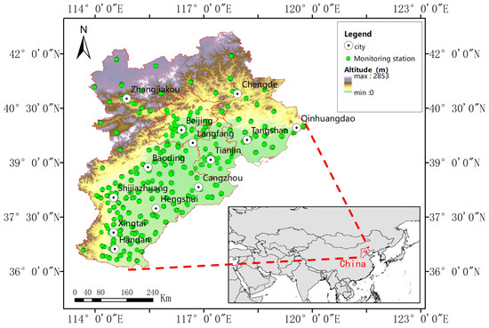
Figure 1.
Distribution of air monitoring stations in Beijing–Tianjin–Hebei region from 2015 to 2022.
The natural factor datasets included data on temperature, precipitation, and solar radiation. The data regarding temperature, precipitation, wind speed, and relative humidity were obtained from 177 monitoring stations at the National Meteorological Science Data Center; the solar radiation data and vegetation index (NDVI) data were obtained from LAADS DAAC (Table 1).

Table 1.
All the source data.
The social factor datasets included data on population density, night light index, and land-use type (Table 1). The population density data were sourced from the world population density data released by WorldPop; the night light data were sourced from the global NPP-VIIRS-like released by Harvard Dataverse. These data spanned 2015–2022, and the spatial resolution was 1 km. The land-use type data were interpreted using the Landsat-8 remote sensing images (30 m resolution) of the United States Landsat. Due to the small annual changes in various land-use types in the study area, the Landsat-8 remote sensing images from 2022 were selected for this study, and we used the CNLUCC method to calculate the area of various land-use types, including cultivated land, forest land, grassland, construction land, water, and unused land.
2.2. Methods
2.2.1. Data Preprocessing and Interpolation Analysis
In this study, the raw data were preprocessed. To ensure the spatial continuity of the data (according to the data regarding known monitoring points, the regional ozone concentration was deduced), we used the Kriging interpolation method to conduct an interpolation analysis of ozone data. Moreover, when using the geodetector, the Jenks natural breaks method was used to transform continuous into categorical factors [21].
2.2.2. Stepwise Regression Analysis
The main advantage of stepwise regression analysis is that it can help to screen out the most important independent variables to avoid overfitting [22,23,24]. By using SPSS for stepwise regression analysis, we analyzed the main factors affecting the seasonal changes in the ozone concentration, which was calculated as follows:
Y = β0 + β1X1 + β2X2 + … + βnXn + ε
In the formula, Y denotes the ozone concentration, β0 denotes the intercept term, Xi (i = 1, 2, 3 … n) denotes the explanatory variables, βi (i = 1, 2, 3 … n) denotes the regression coefficient, and ε denotes the error term.
2.2.3. Geographically Weighted Regression Model
In geographically weighted regression models [25,26,27,28], each location has its unique regression coefficient, reflecting the impact of geographical location on the results, thus allowing the explanation and analysis of the spatial variation in data. In this study, we applied the geographically weighted regression model to explore the spatial differences in the explanatory power of the major factors affecting ozone concentration, which was calculated as follows:
In the formula, y is argument and denotes the monitoring data of ozone concentration, denotes the regression coefficient at point i, indicating the influencing extent of the independent variable on the dependent variable. denotes the geographical location of observation point i. denotes the k-th regression coefficient at point i. denotes the value of independent variable x at point i. p denotes the number of independent variables. is a random error term and represents the normal distribution function with constant variance.
2.2.4. Geographical Detector Analysis
The geographical detector model can be used to detect the spatial heterogeneity of ozone concentration impact factors, thus revealing its underlying driving forces. The factor detection calculation formula is [29]:
In the formula, q is the detection factor and represents the detection force value of the factor on the dependent variable. q ranges from 0 to 1, with a larger q value indicating stronger explanatory power of the factor, and vice versa. N and Nh denote the number of elements in the whole area and layer, respectively. and denote the variances of y values in layer h and the whole area, respectively. L denotes the number of detection partitions.
3. Result and Analysis
3.1. Characteristics of Temporal and Spatial Variations in Ozone Concentration in Jing–Jin–Ji
3.1.1. Characteristics of Seasonal Variation
To ensure the spatial continuity of the data, we used the Kriging interpolation method to conduct an interpolation analysis of ozone data from 2015 to 2022 in the Jing–Jin–Ji region (Figure 2). As shown in Figure 3 and Figure 4, large seasonal differences were found in ozone concentration in the Jing–Jin–Ji region, specifically with levels, in descending order, of summer > spring > autumn > winter. The ozone concentrations in summer and winter were 111.1 and 46.1 µg/m3, respectively. This seasonal trend may be related to various factors. The higher ozone concentrations in summer may have been associated with high temperatures and sufficient sunlight, which promote the formation of ozone. In contrast, the lower ozone concentrations in winter may have been due to the combined effects of cold and dry climate conditions, weakened vertical mixing, insufficient ultraviolet radiation, and NO2 pollution.
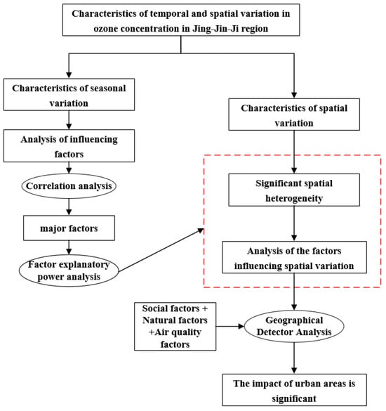
Figure 2.
Research methods.
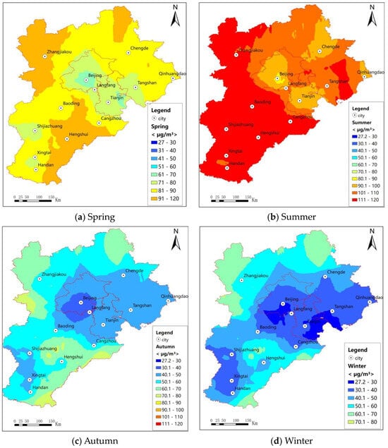
Figure 3.
Seasonal variation of ozone concentration in the Jing–Jin–Ji region from 2015 to 2022.
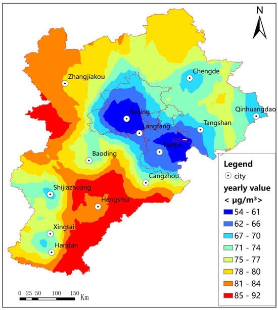
Figure 4.
The mean distribution of ozone in the Jing–Jin–Ji region from 2015 to 2022.
3.1.2. Characteristics of Spatial Variation
In the spatial dimensions, the distribution of ozone concentration differed widely. Specifically, urban central areas usually exhibit lower ozone concentrations, while relatively remote suburban areas show higher ozone concentrations. As shown in Figure 4, the ozone concentration varied from 56.2 to 88.9 µg/m3. In major cities in the Jing–Jin–Ji region, such as Beijing, Tianjin, and Shijiazhuang, the ozone concentration was relatively low, with the lowest value of 56.2 µg/m3 found in the central urban area of Beijing. However, levels of ozone were higher in suburban areas, such as in the southeastern suburbs of Hebei province, where the average ozone concentration was 85 µg/m3 or more. This distribution indicates that ozone concentration showed strong spatial heterogeneity in the Jing–Jin–Ji region.
3.2. Analysis of Influencing Factors on Seasonal Variation of Ozone Concentration
3.2.1. Correlation Analysis
To investigate the effects of different factors on ozone concentration, we conducted a multifactor Spearman correlation analysis of the temporal variation in ozone concentration. We chose meteorological and air quality factors as the focus of our analysis, rather than social factors. This is because social factors would have relatively changed minimally within the time frame of our study, and their patterns affecting the variation in ozone concentration would be different from those of other factors, so we excluded social factors [30]. As shown in Figure 5, the correlation coefficient between temperature and ozone concentration was 0.84, indicating a strong positive correlation between temperature and ozone concentration increases [31]. The correlation coefficient between precipitation and ozone concentration was 0.56, indicating a correlation between precipitation events and the increase in ozone concentration [32,33,34]. Solar radiation and ozone concentration were strongly and positively correlated, with a coefficient of 0.83, suggesting a close association between increased solar radiation and increased ozone concentration. Additionally, the correlation coefficients of PM2.5 and NO2 were −0.32 and −0.44, respectively, indicating a negative correlation with ozone concentration. The correlation coefficients between CO levels, relative humidity, and ozone concentration were close to zero, with p-values greater than 0.05, indicating no correlation among CO levels, relative humidity, and ozone concentration [35,36,37,38,39,40,41,42].
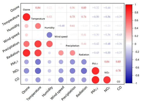
Figure 5.
Correlation between ozone concentration and seasonal variation factors.
3.2.2. Factor Explanatory Power Analysis
To investigate the key factors influencing ozone concentration, a stepwise regression model was employed. In the initial model, we considered the impact of correlated factors on ozone concentration. The expression of this model was as follows: ozone = −1.936 + 1.607 × temperature + 0.000 × solar radiation (F = 61.470, p = 0.000 < 0.05), with an R-squared value of 0.730, indicating that these four factors explained 73.0% of the variation in the ozone concentration. However, the VIF value for temperature was greater than five, indicating a collinearity issue [43]. To optimize the model and address this issue, strongly correlated independent variables were rescreened, resulting in a simplified model including temperature and solar radiation. The specific results are presented in Table 2. The simplified model expression was as follows: ozone = −1.936 + 1.607 × temperature + 0.000 × solar radiation. The model’s R-squared value was 0.679, meaning that temperature and solar radiation explained 67.9% of the variation in the ozone concentration. This suggests that temperature and solar radiation were the dominant factors influencing seasonal changes in ozone concentration. Through the optimization of the stepwise regression model, we successfully identified the key factors affecting ozone levels.

Table 2.
Results of stepwise regression analysis (temperature, precipitation, and solar radiation).
To explore the spatial effect of temperature and solar radiation on ozone concentration, a geographically weighted regression model was applied to analyze the explanatory power of these factors. The results are presented in Figure 6. From an annual average perspective, the explanatory power of changes in temperature and solar radiation on ozone concentration exhibited a characteristic of being higher in urban centers and lower in suburban areas. In Beijing and Tianjin, this explanatory power exceeded 89% in urban centers; in surrounding areas such as Chengde North and Handan Southeast, the explanatory power was less than 51%. This indicated spatial variability in the explanatory power of temperature and solar radiation on ozone concentration.
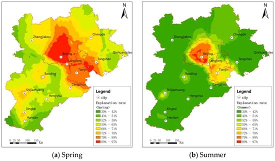
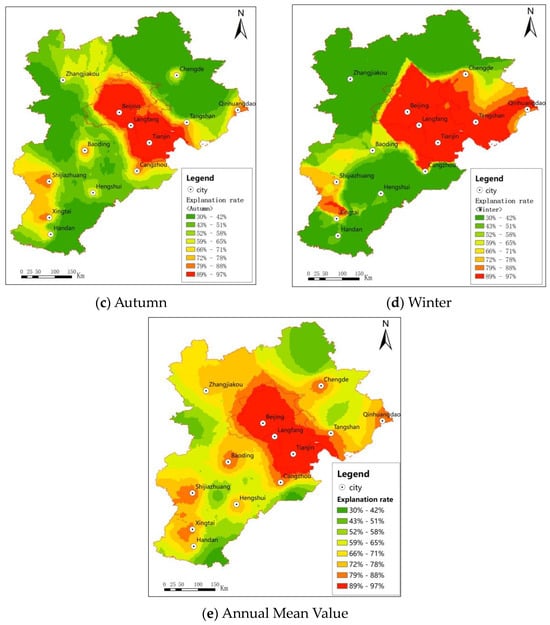
Figure 6.
The explanation ratio of solar radiation and temperature on the variation of ozone concentration.
In terms of seasonal variation, the explanatory power of the factors in spring, summer, autumn, and winter was 66%, 38%, 52%, and 50%, respectively. The explanatory power of temperature and solar radiation was strong in spring and weak in summer, suggesting that temperature and solar radiation strongly influence ozone concentration in spring, with a weaker influence in summer.
3.3. Analysis of Factors Influencing Spatial Variation in Ozone Concentration
3.3.1. Monofactor Exploratory Analysis
The impact of temperature and solar radiation on ozone concentration exhibited considerable spatial variability. To gain a deeper understanding of the underlying factors driving this phenomenon, we employed a geographical detector to conduct a spatial factor analysis of ozone concentration, considering the weights of various geographical factors such as land-use type and precipitation distribution (Figure 7). By elucidating their relative contributions (q-values) in explaining the distribution of ozone concentration, we explored their impact on ozone concentration. The results are presented in Figure 8.
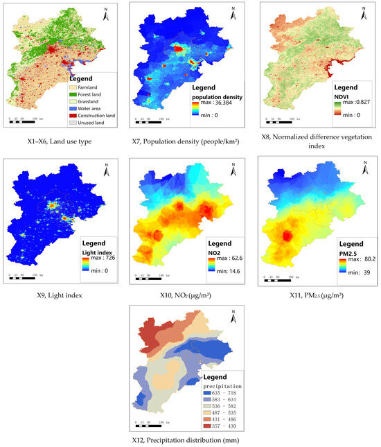
Figure 7.
Various factors in the Jing–Jin–Ji region.
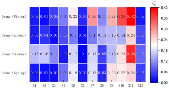
Figure 8.
Influence of various factors on the spatial distribution of ozone (q-value) in the Jing–Jin–Ji region.
From a seasonal perspective, the relative contributions of factors explaining the distribution of ozone concentration were higher in winter, particularly for urban factors (light index, population density, and construction land) and air quality factors (PM2.5 and NO2), which had q-values greater than 0.2. This suggests their strong impact on the spatial variation in ozone concentration, which is consistent with previous research findings [44]. This phenomenon is primarily due to the increased concentration of urban air pollutants in winter. Under unfavorable meteorological conditions, the diffusion of pollutants is limited, and the increased demand for heating promotes higher industrial and residential emissions, leading to a substantial rise in the concentration of pollutants such as NO2 in cities. These pollutants not only directly affect air quality but also influence the formation and distribution of ozone through photochemical reactions and other pathways. In contrast, the contributions of various factors to the spatial distribution of ozone concentration are relatively lower in autumn, with q-values generally below 0.2. This may be due to the favorable autumn climate and atmospheric diffusion conditions, which hinder the accumulation of pollutants. Consequently, the impact of these factors on ozone concentration during autumn is weaker.
Overall, PM2.5 levels most strongly impacted the spatial variations in ozone concentration, with an average q-value of 0.32. This finding is generally consistent with the conclusion of Li et al., based on GEOS-Chem simulations, who primarily attributed the intensification of O3 pollution in the North China Plain to the decrease in PM2.5 levels [45]. Additionally, NO2, as a precursor to ozone formation, also strongly contributed to the spatial distribution of ozone (q = 0.23).
Among the different land-use types, construction land exhibited a relatively high weight (q ≥ 0.1) in the distribution of ozone concentration, highlighting its impact on ozone levels. Construction land is typically located in urban centers, which are more affected by emissions from transportation, industry, and other sources, thereby influencing ozone concentration. The strong impact of urbanization factors on the spatial variation in ozone concentration further corroborates this conclusion.
3.3.2. Two-Factor Interactive Detection Analysis
We analyzed the interactions of 12 influencing factors, and the results (Figure 9) showed that the interaction between any two factors produced bifactor or nonlinear enhancement, with no independent or weakened relationship between them. In other words, the interaction between any two factors created a stronger effect than that created by a single factor, which means that the spatial distribution of ozone in the Jing–Jin–Ji region was influenced by the synergy of multiple factors.
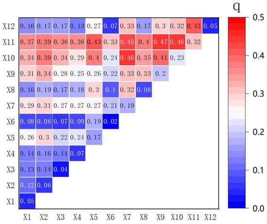
Figure 9.
Interaction of factors driving the spatial distribution of ozone concentration.
The average interaction q-values for the top three combinations of factors that influenced the spatial variations in ozone concentration in the Jing–Jin–Ji urban agglomeration from 2015 to 2022 were light index ∩ PM2.5 (0.47), population density∩NO2 (0.46), and NO2 ∩ PM2.5 (0.46). Additionally, the q-values for the interaction between urban factors (light index, population density, and construction land) and air quality factors (PM2.5 and NO2 levels) ranged from 0.40 to 0.47, indicating a substantially higher impact than the interaction between other influencing factors. This further confirmed their joint impact on ozone concentration. The tight relationship between the light index and population density, which are representative indicators of urban development, and the levels of air pollutants such as PM2.5 and NO2, reflects the impact of urban activities on air quality. This impact may be exerted through various pathways, such as increased emissions sources and the urban heat island effect, which jointly affect the spatial distribution of ozone.
4. Discussion
This study delved into the relationship between various factors influencing seasonal changes in ozone concentration. From the analysis of the results of a stepwise regression model, we identified temperature and solar radiation as the primary factors influencing ozone concentration, which together explained 67.9% of the variance in ozone concentration. This finding is consistent with those of existing studies on the impact of meteorological conditions on ozone formation, further emphasizing the crucial role of meteorological factors in the formation of ozone pollution.
However, analyzing influencing factors solely using a global model may lead to spatial heterogeneity being overlooked. Therefore, we employed a geographically weighted regression model to analyze the spatial impacts of temperature and solar radiation on ozone concentration. The results revealed wide differences in the explanatory power of influencing factors between urban and suburban areas. The dense human activities and numerous emission sources in urban centers led to a stronger impact of temperature and solar radiation on ozone concentration, which could have been related to the urban heat island effect and increased photochemical reactions. In contrast, in the suburbs, with fewer emission sources and a stronger influence from natural conditions, temperature and solar radiation exhibited relatively lower explanatory power.
Additionally, this study found that the explanatory power of the considered influencing factors was substantially affected by the season. In spring, the impact of temperature and solar radiation on ozone concentration was particularly strong, which may have been associated with the rise in temperature, increased solar radiation, and more emission sources. However, in summer, although temperature and solar radiation remained important, their impact was relatively weaker. This may have been related to summer climatic conditions, such as increased precipitation, which helps to clear air pollutants, including ozone precursors.
From the results of geographic detector analysis, we further explored the impact of different seasons and geographic factors on ozone concentration. The results showed that urbanization and air quality factors considerably impacted the ozone concentration in winter, which may have been related to coal-fired heating and an increased number of emission sources. In contrast, the impact of various factors on ozone concentration was relatively weaker in autumn, possibly due to favorable climatic conditions and better atmospheric diffusion, hindering the accumulation of pollutants.
The results of the analysis of the interaction among factors revealed a strong impact of the interaction between urban and air factors on ozone concentration. This finding emphasizes the important role of urban activities in the formation of ozone pollution and the close relationship between air quality factors and urban activities. This provides important insights for developing effective ozone pollution prevention and control strategies. The same pattern has also been observed in other parts of the world. In the United States, the concentration of ozone in urban environments is lower than that in rural areas, which has been attributed to increased ozone titration or sinks in urban areas [46].
In summary, this study emphasizes the crucial role of meteorological, urbanization, and air quality factors in the formation of ozone pollution and reveals the spatial and temporal heterogeneity of these influencing factors. These findings provide an important basis for deeply understanding the mechanism through which ozone pollution is formed and developing effective prevention and control measures. Although important results were obtained in this study, the two following important points need to be addressed in future research:
(1) When analyzing the influencing factors, due to a shortage of data for VOCs and vehicle inventories, we could not explore the magnitude of the influence of these factors on ozone pollution or their relationships. Based on current research, these elements appear to be important factors influencing the formation of ozone pollution.
(2) Although we found that urban areas strongly impacted the ozone concentration, the complex mechanisms of this effect remain unclear. Some urban effects may indirectly affect ozone concentration, such as the heat island effect. The impact of urban factors on the ozone concentration needs to be studied in the future.
5. Conclusions
The ozone concentration in the Jing–Jin–Ji region exhibited substantial temporal and spatial variations. In terms of seasonal changes, the ozone concentration was highest in summer, followed by in spring, autumn, and winter. The maximum was 111.1 µg/m3 in summer and the minimum was 46.1 µg/m3 in winter. In terms of spatial distribution, the ozone concentration was generally lower in urban centers and higher in suburban areas, with a distribution ranging from 56.2 to 88.9 µg/m3.
Regarding the factors influencing seasonal changes, temperature, precipitation, solar radiation, PM2.5 levels, and NO2 levels correlated with ozone concentration. From the results of a stepwise regression model, we determined that temperature and solar radiation were the dominant factors affecting ozone concentration, which together explained 67.9% of the variation. To explore the spatial scale of the effects of these two factors on ozone concentration, we employed a geographically weighted regression model. The results demonstrated spatial variations in the explanatory power of temperature and solar radiation, with higher explanatory rates in urban centers and lower rates in suburban regions. Furthermore, the impact was stronger in spring and weaker in summer.
Utilizing a geographic detector for analysis of the influencing factors, substantial differences in the contribution of various seasonal and geographical factors to ozone concentration were observed. Specifically, in winter, the impact of urbanization and air quality factors on ozone concentration was particularly pronounced, with q-values exceeding 0.2. In contrast, the influence of these factors on ozone concentration was relatively weaker in autumn. Additionally, the q-values for the interaction between urban factors (light index, population density, and construction land) and air quality factors (PM2.5 and NO2 levels) ranged from 0.40 to 0.47, indicating a substantially higher impact than the interaction between other influencing factors, further confirming the important role of urban activities in determining ozone levels.
Author Contributions
All authors contributed to the study conception and design. Data collection and analysis were performed by G.-S.X., Y.L., X.-Z.L., Y.-Z.R. and Q.-Z.T. The first draft of the manuscript was written by G.-S.X., the final draft of the manuscript was reviewed and revised by X.-W.T. and all authors commented on previous versions of the manuscript. All authors have read and agreed to the published version of the manuscript.
Funding
This research was funded by the Science and Technology Project of Hebei Education Department (grant No. BJ2021049), the Foundation of Hebei University of Environmental Engineering (grant No.2023XJKT12) and the S&T Program of Qinhuangdao (202101A103).
Institutional Review Board Statement
Not applicable.
Informed Consent Statement
Not applicable.
Data Availability Statement
All data generated or analyzed during this study are included in this published article.
Conflicts of Interest
The authors declare no conflicts of interest.
References
- Lyu, X.; Li, K.; Guo, H.; Morawska, L.; Zhou, B.; Zeren, Y.; Jiang, F.; Chen, C.; Goldstein, A.H.; Xu, X.; et al. A synergistic ozone-climate control to address emerging ozone pollution challenges. One Earth 2023, 6, 964–977. [Google Scholar] [CrossRef]
- Qi, J.; Mo, Z.; Yuan, B.; Huang, S.; Huangfu, Y.; Wang, Z.; Li, X.; Yang, S.; Wang, W.; Zhao, Y.; et al. An observation approach in evaluation of ozone production to precursor changes during the COVID-19 lockdown. Atmos. Environ. 2021, 262, 118618. [Google Scholar] [CrossRef] [PubMed]
- Lu, Z.; Guan, Y.; Shao, C.; Niu, R. Assessing the health impacts of PM2.5 and ozone pollution and their comprehensive correlation in Chinese cities based on extended correlation coefficient. Ecotoxicol. Environ. Saf. 2023, 262, 115125. [Google Scholar] [CrossRef] [PubMed]
- Silva, P.; Custodio, I.S.; Wainer, I.; Dias, P.L.d.S.; Prado, L.F. Assessment of Tropical Atlantic ocean variability and associated rainfall sensibility due to atmospheric ozone changes. Atmos. Environ. 2022, 290, 119344. [Google Scholar] [CrossRef]
- Woller, S.C.; Horne, B.D.; Stevens, S.M.; Lloyd, J.F.; Bride, D.; Snow, G.L.; Bledsoe, J. Association of Ozone and PM2.5 Air Pollution on Short-Term Venous Thromboembolism Risk, Including 10861 Vte Events in an Integrated Health System: 17 Years of Longitudinal Data. Chest 2023, 164 (Suppl. S4), A5105–A5106. [Google Scholar]
- Liu, J.; Wang, M.; Deng, J.; Chen, X.; Tang, X.; Zeng, L. Temporal and spatial evolution patterns of AQl, particulate matter, and ozone in Shandong province and key influencing factors. Res. Environ. Sci. 2023, 36, 273–284. [Google Scholar]
- Yao, H.; Zhou, J.; Yang, J.; Qu, Z.-G.; Cao, Y.-X. Studies on characteristics of PM2.5, PM10 and ozone pollution in Wuhan based on wavelet transform. China Environ. Sci. 2023, 43, 107–114. [Google Scholar]
- Yang, X.; Lu, Y.; Wang, Y.; Qiao, Y.-H.; Zhang, G.-L.; Wang, S.-G.; Zhang, X.-L.; Liu, Z.-H.; Liu, Y.-L.; Zhu, X.-S. Impact of synoptic patterns on regional ozone pollution in Sichuan Basin. China Environ. Sci. 2021, 41, 2526–2539. [Google Scholar]
- Liu, S.; Huang, Q.; Zhang, X.; Dong, W.; Zhang, W.; Wu, S.; Yang, D.; Nan, B.; Zhang, J.; Shen, H.; et al. Cardiorespiratory Effects of Indoor Ozone Exposure Associated with Changes in Metabolic Profiles among Children: A Repeated-Measure Panel Study. Innovation 2021, 2, 100087. [Google Scholar] [CrossRef] [PubMed]
- Yaluk, E.A.; Wang, Y.; Jiang, S.; Huang, L.; Lu, G.; Zhu, A.; Bian, J.; Xue, J.; Du, Y.; Chen, N.; et al. Changes in first- and second-order sensitivities of ozone concentration to its precursors over the Yangtze River Delta region of China due to COVID-19 lockdown: Insights from CMAQ-HDDM modeling study. Atmos. Environ. 2023, 309, 119931. [Google Scholar] [CrossRef]
- Li, K.; Hayes, F.; Chadwick, D.R.; Wang, J.; Zou, J.; Jones, D.L. Changes in microbial community composition drive the response of ecosystem multifunctionality to elevated ozone. Environ. Res. 2022, 214, 114142. [Google Scholar] [CrossRef] [PubMed]
- Kawano, N.; Nagashima, T.; Sugata, S. Changes in seasonal cycle of surface ozone over Japan during 1980–2015. Atmos. Environ. 2022, 279, 119108. [Google Scholar] [CrossRef]
- Villota, N.; Cruz-Alcalde, A.; Ferreiro, C.; Lombraña, J.I.; Esplugas, S. Changes in solution turbidity and color during paracetamol removal in laboratory and pilot-scale semicontinuous ozonation reactors. Sci. Total Environ. 2023, 854, 158682. [Google Scholar] [CrossRef] [PubMed]
- Meng, X.; Jiang, J.; Chen, T.; Zhang, Z.; Lu, B.; Liu, C.; Xue, L.; Chen, J.; Herrmann, H.; Li, X. Chemical drivers of ozone change in extreme temperatures in eastern China. Sci. Total Environ. 2023, 874, 162424. [Google Scholar] [CrossRef] [PubMed]
- Ban, J.; Lu, K.; Wang, Q.; Li, T. Climate change will amplify the inequitable exposure to compound heatwave and ozone pollution. One Earth 2022, 5, 677–686. [Google Scholar] [CrossRef]
- Li, Y.; Wu, Z.; Ji, Y.; Chen, T.; Li, H.; Gao, R.; Xue, L.; Wang, Y.; Zhao, Y.; Yang, X. Comparison of the ozone formation mechanisms and VOCs apportionment in different ozone pollution episodes in urban Beijing in 2019 and 2020: Insights for ozone pollution control strategies. Sci. Total Environ. 2024, 908, 168332. [Google Scholar] [CrossRef] [PubMed]
- Zhang, L.; Wang, L.; Tang, G.; Xin, J.; Li, M.; Li, X.; Xin, F.; Qin, Y.; Wang, Y.; Hu, B. Comprehensively exploring the characteristics and meteorological causes of ozone pollution events in Beijing during 2013–2020. Atmos. Res. 2023, 294, 106978. [Google Scholar] [CrossRef]
- Liu, L.; Gong, H.; Wang, L.; Chen, W.; Wu, R.; Tao, W.; Dong, Z.; Liu, B. Contribution of atmospheric circulations changes to the variations of summertime lower tropospheric ozone over East Asia during recent decades. Atmos. Res. 2023, 292, 106852. [Google Scholar] [CrossRef]
- Huang, Z.; Luo, M.; Gao, M.; Ning, G.; Ge, E.; Chan, T.O.; Wu, S.; Zhang, H.; Tang, Y. Different characteristics of independent and compound extreme heat and ozone pollution events in the Greater Bay Area of China. Int. J. Appl. Earth Obs. Geoinf. 2023, 124, 103508. [Google Scholar] [CrossRef]
- Wu, K.; Wang, Y.; Qiao, Y.; Liu, Y.; Wang, S.; Yang, X.; Wang, H.; Lu, Y.; Zhang, X.; Lei, Y. Drivers of 2013–2020 ozone trends in the Sichuan Basin, China: Impacts of meteorology and precursor emission changes. Environ. Pollut. 2022, 300, 118914. [Google Scholar] [CrossRef] [PubMed]
- Zhou, C.; Chen, J.; Wang, S. Examining the effects of socioeconomic development on fine particulate matter (PM2.5) in China’s cities using spatial regression and the geographical detector technique. Sci. Total Environ. 2018, 619–620, 436–445. [Google Scholar] [CrossRef] [PubMed]
- Pistore, L.; Pernigotto, G.; Cappelletti, F.; Gasparella, A.; Romagnoni, P. A stepwise approach integrating feature selection, regression techniques and cluster analysis to identify primary retrofit interventions on large stocks of buildings. Sustain. Cities Soc. 2019, 47, 101438. [Google Scholar] [CrossRef]
- Liu, Y.; Heuvelink, G.B.; Bai, Z.; He, P.; Xu, X.; Ding, W.; Huang, S. Analysis of spatio-temporal variation of crop yield in China using stepwise multiple linear regression. Field Crops Res. 2021, 264, 108098. [Google Scholar] [CrossRef]
- Pourshoaib, S.J.; Ghatrami, E.R.; Shamekhi, M.A. Comparing ultrasonic- and microwave-assisted methods for extraction of phenolic compounds from Kabkab date seed (Phoenix dactylifera L.) and stepwise regression analysis of extracts antioxidant activity. Sustain. Chem. Pharm. 2022, 30, 100871. [Google Scholar] [CrossRef]
- Chen, L.; Zhong, Q.; Li, Z. Analysis of spatial characteristics and influence mechanism of human settlement suitability in traditional villages based on multi-scale geographically weighted regression model: A case study of Hunan province. Ecol. Indic. 2023, 154, 110828. [Google Scholar] [CrossRef]
- Senyel Kurkcuoglu, M.A. Analysis of the energy justice in natural gas distribution with Multiscale Geographically Weighted Regression (MGWR). Energy Rep. 2023, 9, 325–337. [Google Scholar] [CrossRef]
- Feng, Z.; Xu, C.; Zuo, Y.; Luo, X.; Wang, L.; Chen, H.; Xie, X.; Yan, D.; Liang, T. Analysis of water quality indexes and their relationships with vegetation using self-organizing map and geographically and temporally weighted regression. Environ. Res. 2023, 216, 114587. [Google Scholar] [CrossRef] [PubMed]
- Carlucci, M.; Salvati, L. Assessing path-dependent urban growth with geographically weighted regressions. Environ. Impact Assess. Rev. 2023, 98, 106920. [Google Scholar] [CrossRef]
- Ding, Y.; Zhang, M.; Qian, X.; Li, C.; Chen, S.; Wang, W. Using the geographical detector technique to explore the impact of socioeconomic factors on PM2.5 concentrations in China. J. Clean. Prod. 2019, 211, 1480–1490. [Google Scholar] [CrossRef]
- Malashock, D.A.; Delang, M.N.; Becker, J.S.; Serre, M.L.; West, J.J.; Chang, K.-L.; Cooper, O.R.; Anenberg, S.C. Global trends in ozone concentration and attributable mortality for urban, peri-urban, and rural areas between 2000 and 2019: A modelling study. Lancet Planet. Health 2022, 6, e958–e967. [Google Scholar] [CrossRef] [PubMed]
- Hu, C.; Kang, P.; Jaffe, D.A.; Li, C.; Zhang, X.; Wu, K.; Zhou, M. Understanding the impact of meteorology on ozone in 334 cities of China. Atmos. Environ. 2021, 248, 118221. [Google Scholar] [CrossRef]
- Li, J.; Cai, J.; Zhang, M.; Liu, H.; Han, X.; Cai, X.; Xu, Y. Model analysis of meteorology and emission impacts on springtime surface ozone in Shandong. Sci. Total Environ. 2021, 771, 144784. [Google Scholar] [CrossRef] [PubMed]
- Pratap, V.; Kumar, A.; Singh, A.K. Overview of solar eclipse of 21st June 2020 and its impact on solar irradiance, surface ozone and different meteorological parameters over eight cities of India. Adv. Space Res. 2021, 68, 4039–4049. [Google Scholar] [CrossRef]
- Gao, Z.; Ivey, C.E.; Blanchard, C.L.; Do, K.; Lee, S.-M.; Russell, A.G. Separating emissions and meteorological impacts on peak ozone concentrations in Southern California using generalized additive modeling. Environ. Pollut. 2022, 307, 119503. [Google Scholar] [CrossRef] [PubMed]
- Feng, Z.; Kobayashi, K.; Li, P.; Xu, Y.; Tang, H.; Guo, A.; Paoletti, E.; Calatayud, V. Impacts of current ozone pollution on wheat yield in China as estimated with observed ozone, meteorology and day of flowering. Atmos. Environ. 2019, 217, 116945. [Google Scholar] [CrossRef]
- Cleary, P.A.; Dickens, A.; McIlquham, M.; Sanchez, M.; Geib, K.; Hedberg, C.; Hupy, J.; Watson, M.W.; Fuoco, M.; Olson, E.R.; et al. Impacts of lake breeze meteorology on ozone gradient observations along Lake Michigan shorelines in Wisconsin. Atmos. Environ. 2022, 269, 118834. [Google Scholar] [CrossRef] [PubMed]
- Chang, J.H.; Griffith, S.M.; Lin, N. Impacts of land-surface forcing on local meteorology and ozone concentrations in a heavily industrialized coastal urban area. Urban Clim. 2022, 45, 101257. [Google Scholar] [CrossRef]
- Zhu, X.; Ma, Z.; Li, Z.; Wu, J.; Guo, H.; Yin, X.; Ma, X.; Qiao, L. Impacts of meteorological conditions on nocturnal surface ozone enhancement during the summertime in Beijing. Atmos. Environ. 2020, 225, 117368. [Google Scholar] [CrossRef]
- Xu, B.; Wang, T.; Gao, L.; Ma, D.; Song, R.; Zhao, J.; Yang, X.; Li, S.; Zhuang, B.; Li, M.; et al. Impacts of meteorological factors and ozone variation on crop yields in China concerning carbon neutrality objectives in 2060. Environ. Pollut. 2023, 317, 120715. [Google Scholar] [CrossRef] [PubMed]
- Sánchez-Ccoyllo, O.R.; Ynoue, R.Y.; Martins, L.D.; Andrade, M.d.F. Impacts of ozone precursor limitation and meteorological variables on ozone concentration in São Paulo, Brazil. Atmos. Environ. 2006, 40, 552–562. [Google Scholar] [CrossRef]
- Godowitch, J.M.; Gilliam, R.C.; Roselle, S.J. Investigating the impact on modeled ozone concentrations using meteorological fields from WRF with an updated four–dimensional data assimilation approach. Atmos. Pollut. Res. 2015, 6, 305–311. [Google Scholar] [CrossRef]
- Li, K.; Chen, L.; Ying, F.; White, S.J.; Jang, C.; Wu, X.; Gao, X.; Hong, S.; Shen, J.; Azzi, M.; et al. Meteorological and chemical impacts on ozone formation: A case study in Hangzhou, China. Atmos. Res. 2017, 196, 40–52. [Google Scholar] [CrossRef]
- Wang, M.; Wright, J.; Brownlee, A.; Buswell, R. A comparison of approaches to stepwise regression on variables sensitivities in building simulation and analysis. Energy Build. 2016, 127, 313–326. [Google Scholar] [CrossRef]
- Kong, L.; Zhou, L.; Chen, D.; Luo, L.; Xiao, K.; Chen, Y.; Liu, H.; Tan, Q.; Yang, F. Atmospheric oxidation capacity and secondary pollutant formation potentials based on photochemical loss of VOCs in a megacity of the Sichuan Basin, China. Sci. Total Environ. 2023, 901, 166259. [Google Scholar] [CrossRef] [PubMed]
- Li, K.; Jacob, D.J.; Liao, H.; Shen, L.; Zhang, Q.; Bates, K.H. Anthropogenic drivers of 2013–2017 trends in summer surface ozone in China. Proc. Natl. Acad. Sci. USA 2019, 116, 422–427. [Google Scholar] [CrossRef] [PubMed]
- Ghahremanloo, M.; Choi, Y.; Lops, Y. Deep learning mapping of surface MDA8 ozone: The impact of predictor variables on ozone levels over the contiguous United States. Environ. Pollut. 2023, 326, 121508. [Google Scholar] [CrossRef] [PubMed]
Disclaimer/Publisher’s Note: The statements, opinions and data contained in all publications are solely those of the individual author(s) and contributor(s) and not of MDPI and/or the editor(s). MDPI and/or the editor(s) disclaim responsibility for any injury to people or property resulting from any ideas, methods, instructions or products referred to in the content. |
© 2024 by the authors. Licensee MDPI, Basel, Switzerland. This article is an open access article distributed under the terms and conditions of the Creative Commons Attribution (CC BY) license (https://creativecommons.org/licenses/by/4.0/).