Abstract
Forecasting air quality plays a crucial role in preventing and controlling air pollution. It is particularly significant for improving preparedness for heavily polluted weather conditions and ensuring the health and safety of the population. In this study, a novel deep learning model for predicting air quality spatio-temporal variations is introduced. The model, named graph long short-term memory with multi-head attention (GLSTMMA), is designed to capture the temporal patterns and spatial relationships within multivariate time series data related to air quality. The GLSTMMA model utilizes a hybrid neural network architecture to effectively learn the complex dependencies and correlations present in the data. The extraction of spatial features related to air quality involves the utilization of a graph convolutional network (GCN) to collect air quality data based on the geographical distribution of monitoring sites. The resulting graph structure is imported into a long short-term memory (LSTM) network to establish a Graph LSTM unit, facilitating the extraction of temporal dependencies in air quality. Leveraging a Graph LSTM unit, an encoder-multiple-attention decoder framework is formulated to enable a more profound and efficient exploration of spatio-temporal correlation features within air quality time series data. The research utilizes the 2019–2021 multi-source air quality dataset of Qinghai Province for experimental assessment. The results indicate that the model effectively leverages the impact of multi-source data, resulting in optimal accuracy in predicting six air pollutants.
1. Introduction
The foundation of human survival, reproduction, and healthy development relies on high-quality air conditions [1,2]. In recent years, the rapid progress of global industrialization and urbanization has led to an enhancement in people’s living standards. However, this progress has also resulted in a range of air quality issues [3]. Air pollutants, including carbon monoxide (CO), sulfur dioxide (SO2), volatile organic compounds (VOCs), ozone (O3), and respirable particulate matter (PM2.5 and PM10), are known to be associated with respiratory illnesses, cardiovascular diseases, and cancers [4,5,6]. Simultaneously, specific pollutants have the potential to worsen climate change, jeopardizing human life quality and the sustainable development of society [7,8,9]. The effective and accurate implementation of air pollution prevention and control has emerged as a prominent topic and a significant research area globally [10,11,12]. To enhance air quality effectively, the Chinese government has emphasized the importance of advancing the coordinated control of fine particulate matter and O3. Additionally, there is a need to enhance the capacity for regional ambient air quality prediction and forecasting [13,14]. Therefore, investigating air quality forecasting, enhancing the accuracy of air quality predictions, and encouraging the intelligent utilization of monitoring data can offer dependable technical assistance for crafting effective management tactics for preventing and controlling air pollution in China. This endeavor holds significant importance for the precise regulation of atmospheric environmental pollution and the efficient enhancement of air quality [15,16,17].
Table 1 presents a list of abbreviations and terminologies employed in the paper, along with their corresponding units where appropriate.

Table 1.
Abbreviations and nomenclature.
In the current era of increased integration and extensive advancement of big data and artificial intelligence, alongside the progressive enhancement of China’s ecological monitoring system, and the widespread adoption of the Internet of Things (IoTs) and sensor technologies, the methodologies for predicting air quality are evolving towards diversification, intelligence, and precision [18,19,20]. Traditional methods for predicting air quality encompass numerical prediction, statistical prediction, and machine learning [19,20,21]. Numerical prediction in the field of atmospheric dynamics is grounded in theoretical principles. It utilizes various models such as Gaussian models (ISC3, AERMOD, ADMS [22]), Lagrangian models (OZIP/EKMA [23], CALPUFF [24]), acid deposition models (RADM, ADOM [25]), and coupled dynamo-chemical models (CMAQ [26], NAQPMS [27]) as the core framework. These models integrate meteorological data with pollutant emission inventories to streamline the processes involved in the emission, transport, diffusion, chemical transformations, and removal mechanisms of atmospheric pollutants. Ultimately, this approach enables the spatial and temporal forecasting of air quality [28]. Statistical prediction, in contrast, disregards the physical and chemical transport characteristics of pollutants. It relies on historical meteorological and air quality data and employs statistical models [29] such as multiple linear regression (MLR [30]) and autoregressive integrated moving average (ARIMA [31]) models to predict future pollutant concentrations. Machine learning exhibits an adaptive capacity that is absent in traditional numerical prediction techniques. It has the capability to discern nonlinear correlations within air quality data, a feature that sets it apart from statistical prediction methods. Furthermore, through algorithms like regression, classification, and clustering, machine learning can automatically scrutinize and enhance models based on the data, ultimately leading to heightened prediction precision [32].
The prediction of air quality presents a multivariate spatio-temporal series forecasting challenge, encompassing temporal interdependence, spatial correlation, and diverse information attributes [33]. The primary limitation of conventional methods for predicting air quality lies in the challenge of capturing intricate high-dimensional relationships and spatio-temporal properties of extensive data [34]. Deep learning possesses a potent capability to extract sophisticated and intricate features and acquire knowledge from extensive datasets, thereby increasingly establishing itself as a prominent technical instrument in the realm of air quality forecasting [35]. Recently, two primary categories of deep learning models utilized for the anticipation of air quality have emerged. The first category involves models that utilize a recurrent neural network (RNN), a long short-term memory (LSTM) network, or a gated recurrent unit (GRU) to capture temporal information. These models establish a nonlinear correlation between multivariate time series data and the forecasted pollutant levels [36,37,38]. The primary focus of these studies is on predicting the data from individual monitoring stations, overlooking the interrelation between multiple stations in adjacent areas. Therefore, an enhanced approach involves incorporating spatial networks including a convolutional neural network (CNN) or a graph convolutional network (GCN) onto the temporal model to capture spatio-temporal information [39,40], thereby enhancing prediction accuracy.
In studies focusing on the spatio-temporal prediction of air quality, a persistent challenge lies in the aggregation and integration of spatial site information. Additionally, addressing the issue of information attenuation in time series models when handling extensive datasets poses a significant obstacle. To address the aforementioned issues, this research introduces a deep learning model for graph long-short time memory (Graph LSTM) that incorporates a multi-head attention mechanism. The air sites are depicted as nodes within the graph, with node weights determined by the inter-site distance. The graph’s structure is established based on meteorological and POI data serving as node features. Integrating a graph convolution network (GCN) and a long-short-term memory network (LSTM) enables efficient learning of node features within the graph structure and extraction of spatial correlation information. The graph convolution operator captures long-term dependencies in time series through LSTM network. This approach is applied to air quality prediction at state-controlled sites in Qinghai Province, China, yielding favorable results. This study’s contribution can be outlined as follows:
- The development of an information-rich graph neural network is achieved through the integration of multi-source and heterogeneous data. The model establishes a topology that mirrors the spatial interconnection of the stations by utilizing the geographic coordinates of the air quality monitoring stations. It integrates various types of data from each location, such as air quality data, meteorological data, and POI data in the vicinity, to create a feature matrix that enhances the characterization of the graph neural network.
- This study proposes a model for air quality prediction by integrating GCN and LSTM networks using a multi-head attention mechanism. The model employs graph convolution to capture spatial correlations, substitutes matrix multiplication in RNN with graph convolution operators, and enhances the fusion and extraction of spatio-temporal features of air quality through an encoder-multiple-head attentional decoder architecture to capture temporal dependencies in long sequences for crucial feature inputs.
- The experimental results demonstrate that the model surpasses existing methods in terms of performance, leading to an enhancement in prediction accuracy.
The structure of this paper is as follows. Section 2 provides a comprehensive review of existing research achievements and progress in the field of air quality forecasting. Section 3 elaborates on the multi-source air quality dataset employed in this study and the data preprocessing methods, ensuring the quality and reliability of the experimental data. Section 4 focuses on elucidating the architecture and mathematical formulation of the innovative deep learning model GLSTMMA proposed in this study. Section 5 conducts a comprehensive evaluation of the GLSTMMA model using the multi-source air quality dataset from Qinghai Province spanning 2019 to 2021. Comparative analyses with other mainstream baseline models are performed, and thorough discussions of the obtained results are provided. Section 6 summarizes the research contents and presents an outlook on potential future applications.
2. Related Work
2.1. Traditional Air Quality Prediction Methods
Traditional air quality forecasting methods primarily fall into three categories: numerical prediction, statistical prediction, and machine learning methods. Numerical prediction involves the computational estimation of atmospheric pollutants by solving the conservation of matter equation, aiming to replicate a realistic atmospheric setting [41]. Dennis et al. [42] utilized the regional acid deposition model (RADM) to simulate tropospheric conditions in the eastern United States. This model enables each cell to mimic the chemical transformations of pollutants in the atmosphere, including the cloud formation process. Hu et al. [43] conducted a one-year air quality simulation in China by employing the weather research and forecasting (WRF) model and community multiscale air quality (CMAQ) model. This study aimed to offer comprehensive spatial and temporal data on O3, PM2.5, and various chemical constituents. Numerical prediction models are associated with challenges such as complex operations, high hardware and equipment costs, and extended operational durations. Statistical modeling and machine learning, conversely, exhibit significant simplicity. Lei et al. [44] developed a statistical prediction model for atmospheric particulate matter in Macao with a confidence level of 95% through the application of multiple regression (MR) analysis. Their study revealed that potential height and mean relative humidity significantly impacted the forecasted concentration of particulate matter for the following day. Kumar et al. [45] employed ARIMA and various machine learning models, including linear regression, neural network regression, and decision trees, to examine and forecast the dispersion pattern of respirable suspended particulate matter (RSPM). One of the primary advantages of machine learning methods compared to classical statistical methods lies in their capability to effectively handle nonlinear features. Liu et al. [46] integrated principal component analysis (PCA) and clustering techniques to identify pollutant variables and patterns as significant predictive factors for PM2.5 concentration in support vector regression (SVR), multivariate nonlinear regression (MNR), and artificial neural network (ANN) models. Their study revealed that the SVR model exhibited exceptional forecasting precision. Additionally, they employed a cuckoo search (CS) algorithm for optimization to develop a high-accuracy cuckoo search support vector regression (CSSVR) forecasting model. Their study achieved high forecasting accuracy by optimizing the CSSVR forecasting model using the CS algorithm. However, machine learning techniques have constraints in capturing intricate and nonlinear spatio-temporal correlations, making them insufficient for forecasting complex, dynamic, and data-intensive air quality.
2.2. Deep Learning-Based Air Quality Prediction Methods
Deep learning can effectively extract valuable information from large datasets by enhancing the number of nonlinear feature transformations applied to the original data features. This approach aims to enhance the learning efficacy of the model. Currently, there are two primary categories of air quality forecasting models that leverage deep learning techniques: models that emphasize temporal aspects and models that focus on spatio-temporal aspects. Athira et al. [36] predicted the pollutant PM10 by employing a blend of RNN, LSTM, and GRU. Krishan et al. [47] amalgamated five combinations of factors and parameters, including vehicle emissions, meteorological conditions, traffic data, and pollutant levels, utilizing a two-layer LSTM model to adeptly capture long-term dependencies in modeling air quality parameters. Li et al. [48] proposed a spatio-temporal deep learning (STDL) model that leverages a stacked self-encoder (SAE) model to extract intrinsic features related to air quality. Yan et al. [49] devised a CNN-LSTM prediction model for air quality in Beijing, which incorporates multi-temporal and multi-site data. Their approach involves clustering seasonal air quality data from various sites with the corresponding spatial information. To enhance the representation of air quality site distribution in non-Euclidean space, Chen et al. [50] introduced a group-aware graph neural network (GAGNN) based on a hierarchical model for predicting urban air quality in China. Wang et al. [51] proposed the dynamic adjacency matrix as a graph convolutional layer and presented a spatio-temporal dynamic graph convolutional neural network (ST-DGCNN) to capture the latent and temporally varying spatial dependencies. Zhao et al. [52] employed an integrated method for air quality prediction by combining an air quality spatio-temporal network (AQSTN) characterization model with a GCNN model. Jin et al. [53] proposed a predictive model for PM2.5 time series utilizing a spatio-temporal graph neural network with self-optimization capabilities, referred to as BGGRU. Tang et al. [54] put forward a PM2.5 concentration prediction model that synergistically combines the time-frequency domain, bidirectional long short-term memory, and attention mechanisms. Ding et al. [55] proposed a hybrid model that integrates explainable neural networks and graph neural networks. Hu et al. [56] devised a joint deep learning network framework to facilitate edge-assisted PM2.5 prediction across multiple cities.
In summary, the methods mentioned above do not account for the impact of spatio-temporal correlation, lack the detailed dynamics of long-term dependencies in time series, and overlook the topology of actual geospatial space or the integration of temporal and spatial characteristics through different sub-modules.
3. Data and Pre-Processing
This study develops an air quality dataset through the integration of air quality data, meteorological data, and POI data. The subsequent section provides a comprehensive description of each category of data.
3.1. Air Quality Data
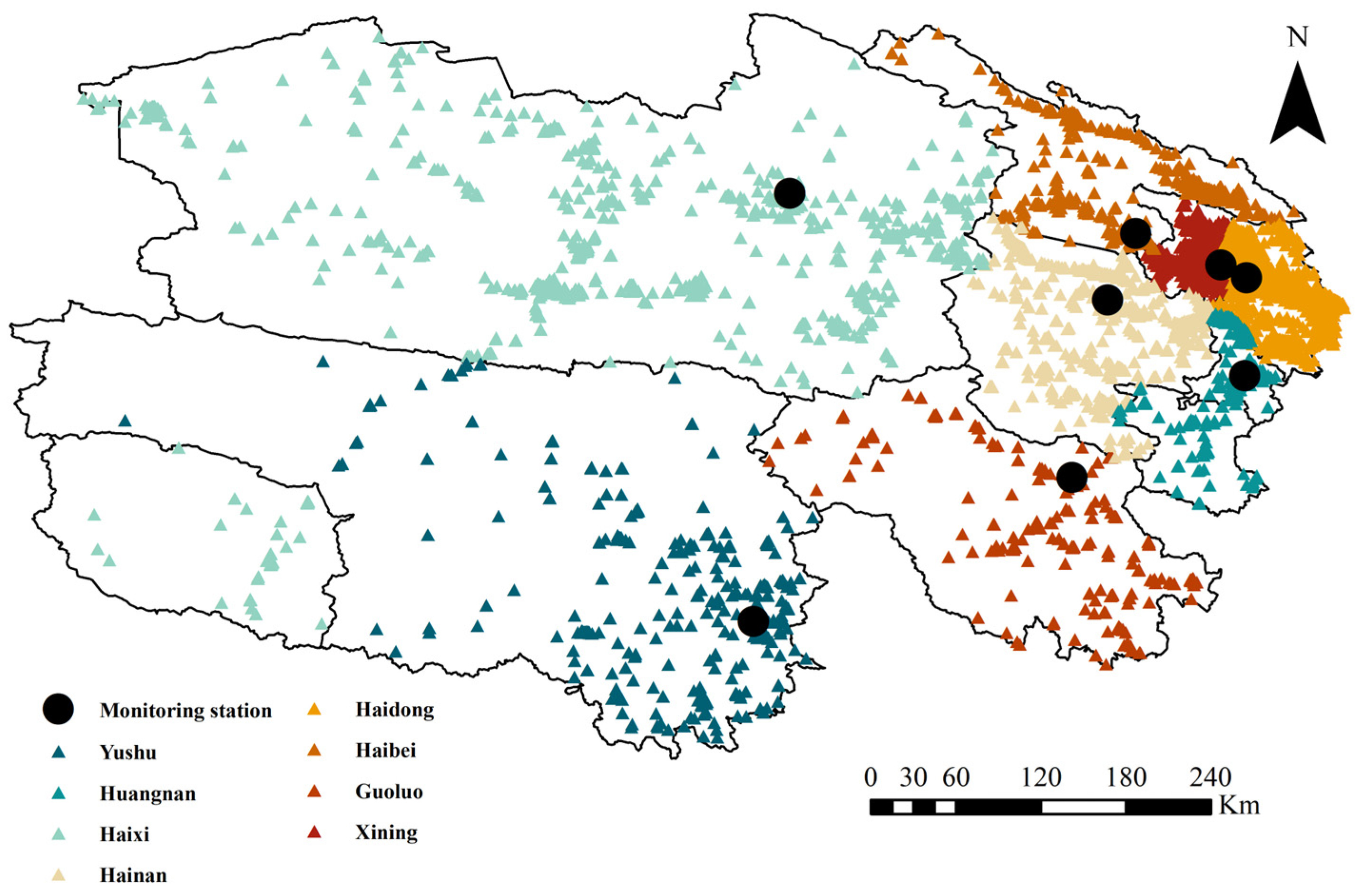
The China National Environmental Monitoring Center (CNEMC) is responsible for China’s environmental monitoring mission and can provide real-time air quality monitoring data from all provinces and cities in China. The data are collected from environmental monitoring stations nationwide and undergo rigorous quality control and data auditing before being publicly disseminated. Consequently, this dataset is widely regarded as one of the most authoritative and frequently utilized resources for contemporary air quality research in China. The data for this study were sourced from the China Urban Air Quality Real-Time Dissemination Platform (CUAQRDP) overseen by the China General Environmental Monitoring Station (CGEMS). The dataset included hourly observations of six air quality parameters: PM2.5, PM10, nitrogen dioxide (NO2), O3, SO2, and CO, as well as air quality index (AQI) data from eight state-controlled stations in Qinghai Province, China (Figure 1). The data spanned from 2019 to 2021.
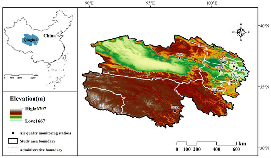
Figure 1.
Geographical distribution of state-controlled ambient air monitoring stations in Qinghai Province.
3.1.1. Missing Value Interpolation
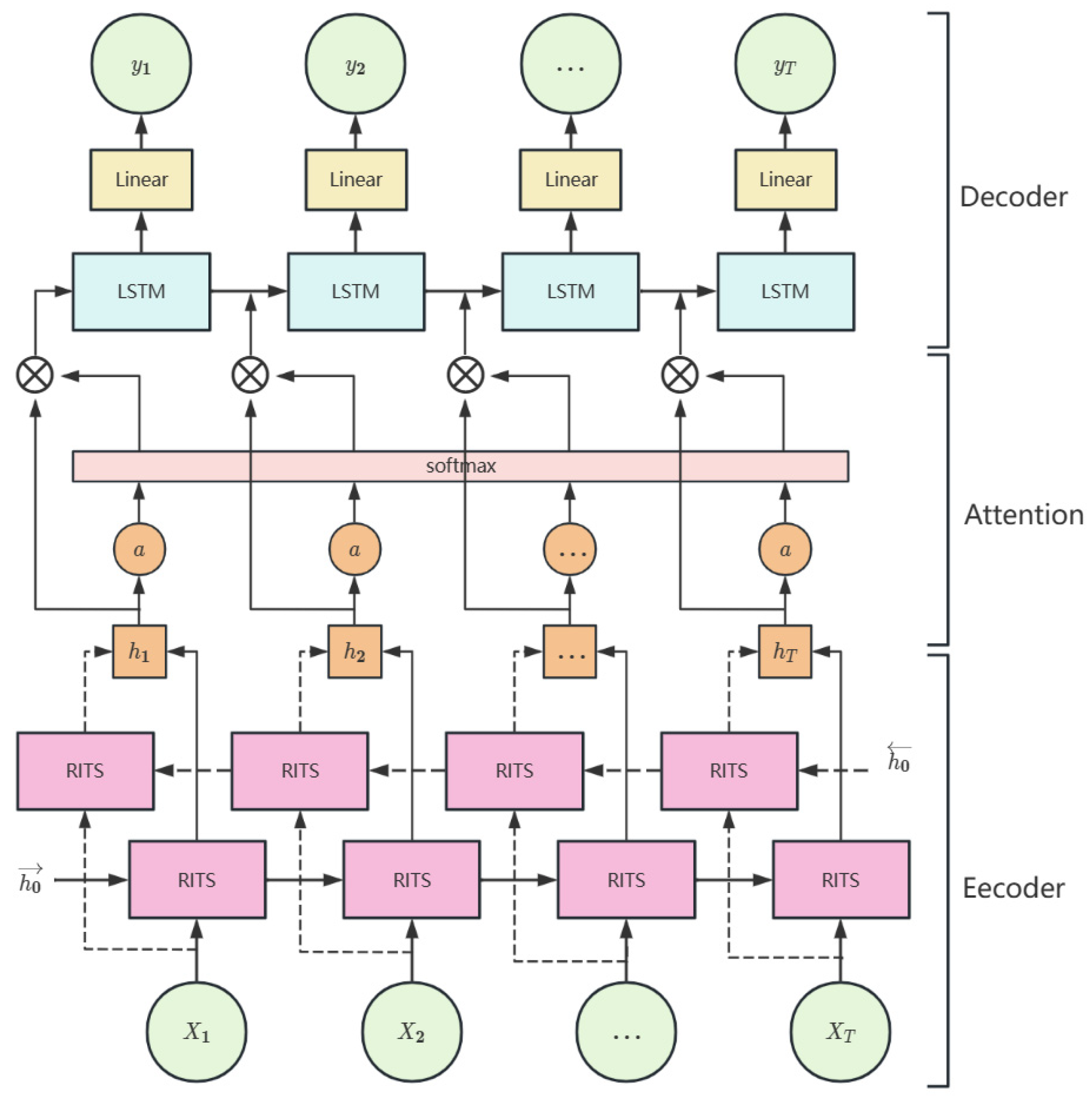
The analysis revealed that the dataset had a missing rate of approximately 5%, rendering it ineffective for air quality prediction. In this investigation, a bidirectional recurrent imputation for time series–attention long short-term memory (BRITS–ALSTM) model for interpolating missing values is developed using a deep learning approach. The model’s architecture is illustrated in Figure 2 [57]. The encoder utilizes BRITS to integrate single-site historical features and multi-site correlation features from the observed data. Subsequently, the decoder establishes the attention mechanism within the hidden state of LSTM to effectively leverage the past information from the observed data for generating hourly interpolation results of missing values in the air quality data.

Figure 2.
BRITS–ALSTM structure for missing value imputation in air quality data.
The missing data for PM2.5, PM10, O3, NO2, SO2, and CO from eight state-controlled stations in Qinghai Province for the years 2019–2021 were interpolated. The results are presented in Table 2. The BRITS–ALSTM model demonstrated superior accuracy compared to traditional methods like mean padding and linear interpolation across all scenarios. This model effectively enhances the robustness and accuracy of air quality prediction models.
Table 2.
Comparison of interpolation results in air quality data.
3.1.2. Spatial Correlation Analysis
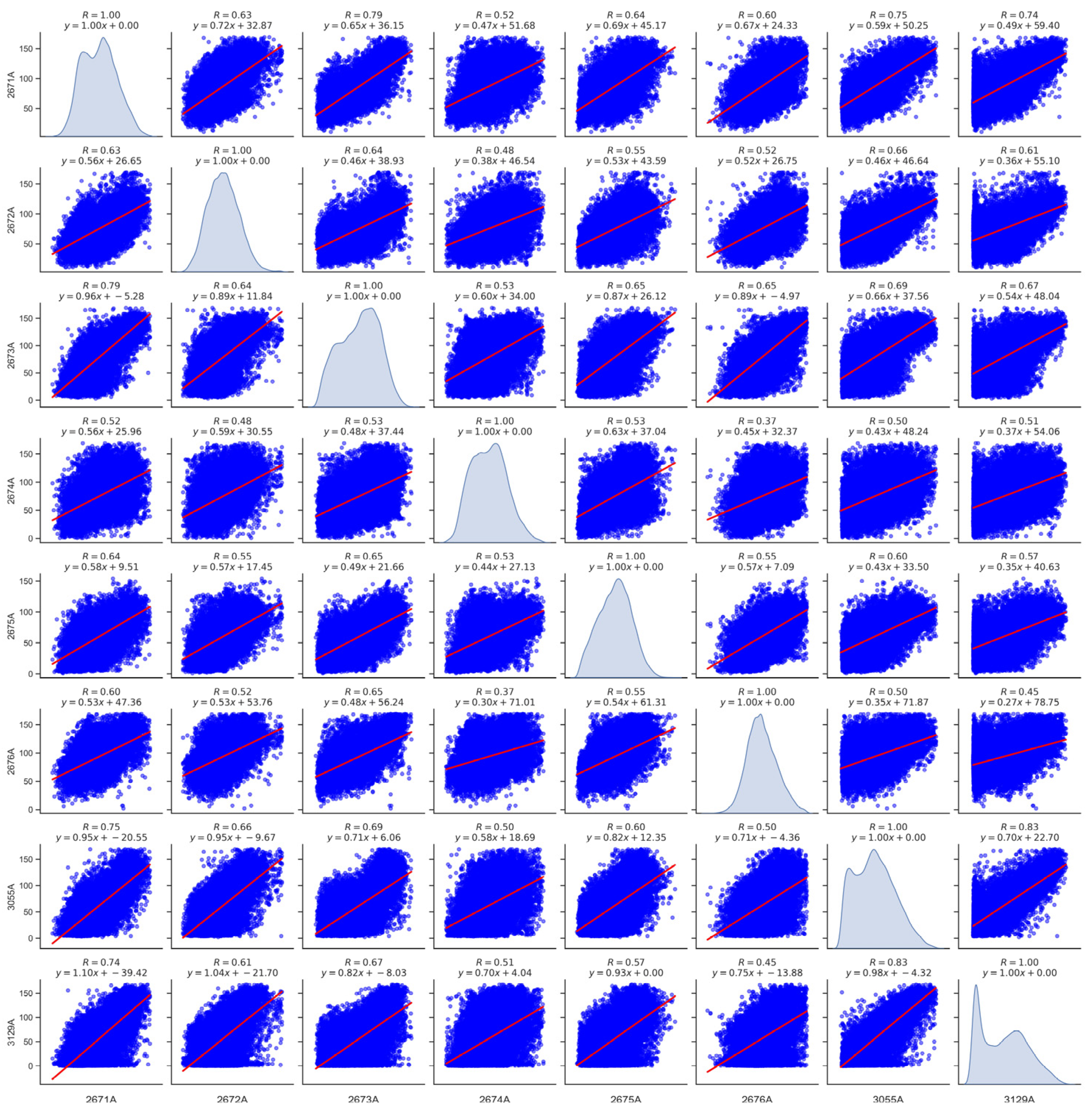
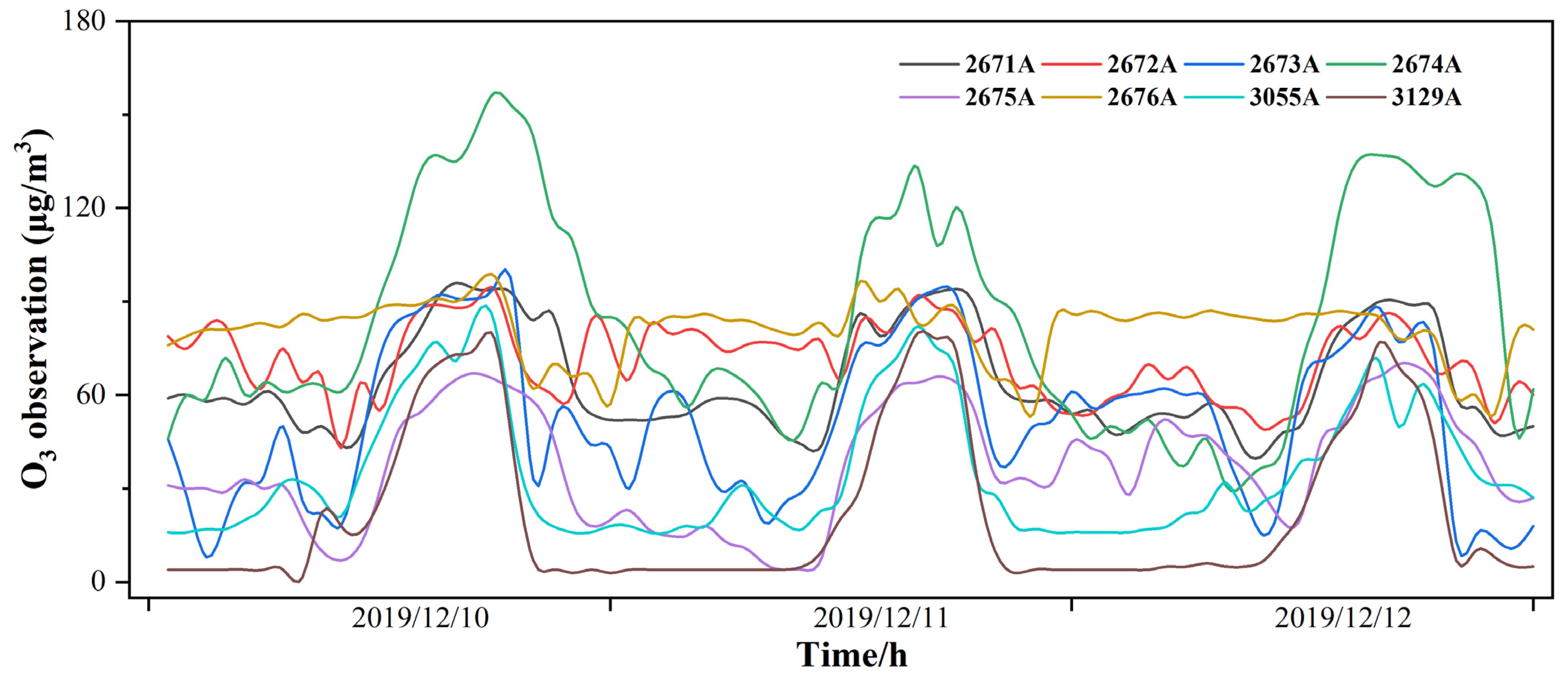
According to the study on multi-site air quality prediction, it has been observed that incorporating historical data from neighboring stations can help mitigate the prediction error to a certain extent. In this study, the air quality data of PM2.5, PM10, O3, NO2 SO2, CO, and AQI from eight state-controlled monitoring stations during the period of 2019–2021 were analyzed for correlations. Taking O3 as an example, Figure 3 illustrates varying degrees of spatial dependence among stations located in different geospatial regions [58]. Air pollutants exhibit propagation in geospatial space, with a stronger correlation observed between stations in closer proximity. However, O3 concentration levels at the remote sites 2675 A and 2676 A also exhibit time-dependent trends closely resembling those observed at the other monitoring locations (Figure 4). This similarity implies the presence of underlying factors that consistently impact the levels of air pollutants. Consequently, incorporating historical data on air pollutants in the vicinity of the sites, variations in pollutant levels at distant locations, and POI data describing the environmental conditions surrounding the sites into the model can enhance prediction accuracy. This approach aims to achieve more precise spatial and temporal forecasts of air quality.

Figure 3.
Correlation heat map of O3 monitoring stations in Qinghai Province. The blue points correspond to simultaneous observations from two stations, while the red line represents the fitted relationship between these stations.

Figure 4.
Comparison of observed values at O3 monitoring stations in Qinghai Province.
3.2. Meteorological Data
Meteorological conditions play a crucial role in influencing air quality. For instance, warmer temperatures can lead to chemical reactions that increase the production of pollutants, while variations in wind direction and speed can impact the dispersion of pollutants. ERA5 is a fifth-generation atmospheric reanalysis dataset that covers global climate data from January 1950 to the present. This dataset is developed by the European Center for Medium-Range Weather Forecasts (ECMWF) and is generated by the ECMWF’s Copernicus Climate Change Service (C3S). ERA5 offers hourly estimates of numerous atmospheric, terrestrial, and oceanic climate parameters with a high level of spatial and temporal detail. For this investigation, seven meteorological data variables were chosen from ERA5 reanalysis dataset spanning the years 2019 to 2021. These variables include 2 m temperature (T2M), wind direction (WD), wind speed (WS), surface pressure (SP), total precipitation (TP), boundary layer height (BLH), and relative humidity (RH). The detailed specifications of the download are presented in Table 3.
Table 3.
Description of meteorological data.
3.3. POI Data
Source apportionment studies of measured air pollutants, such as black carbon, PM2.5, and PM10, have revealed that the major emission sources of these pollutants are influenced by factors including industrial production, vehicular exhaust, and biomass burning [59,60,61]. The spatial distribution of these different emission sources has varying impacts on regional air quality. POI data can provide a range of location-specific information within geospatial contexts, such as land utilization, physical industrial layout, and other related aspects. The data can convey details on traffic flow, including major roads, transportation hubs, and parking lots, as well as information on industrial emissions, such as industrial zones and factories, and green coverage data, such as parks, plazas, and green belts. In this research, POI data serve as supplementary data for predicting air quality. POI data were sourced from the e-map Gaode API, and the distribution of POIs in each city and state are illustrated in Figure 5. The processing procedure for POI data are outlined as follows:
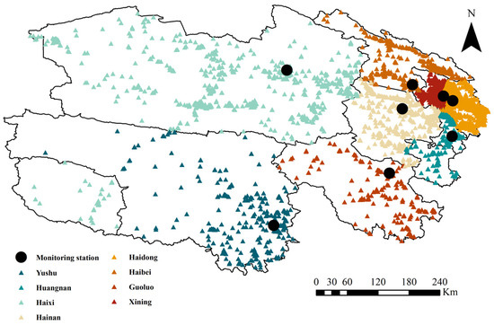
Figure 5.
Distribution of POIs in cities and states of Qinghai Province.
The acquired POI data underwent reclassification from the initial 14 categories to 12 categories, which include industrial factories, agricultural and animal husbandry companies, corporate enterprises, restaurants and cuisines, shopping and consumption, transportation facilities, residences, science, education and culture, tourist attractions, vehicular services, life and medical care, and sports and recreation. The quantity of each of the 12 categories of POIs within the 5 km2 circular buffer zone surrounding the eight sites was tallied as POI features. For any given site s, the statistical equation for POI features is presented as follows:
where denotes POI characteristics of the monitoring site s; p denotes a certain type of POI; denotes i types of POI in the table; and count denotes the method of counting POI numbers.
4. GLSTMMA Network
4.1. Overview
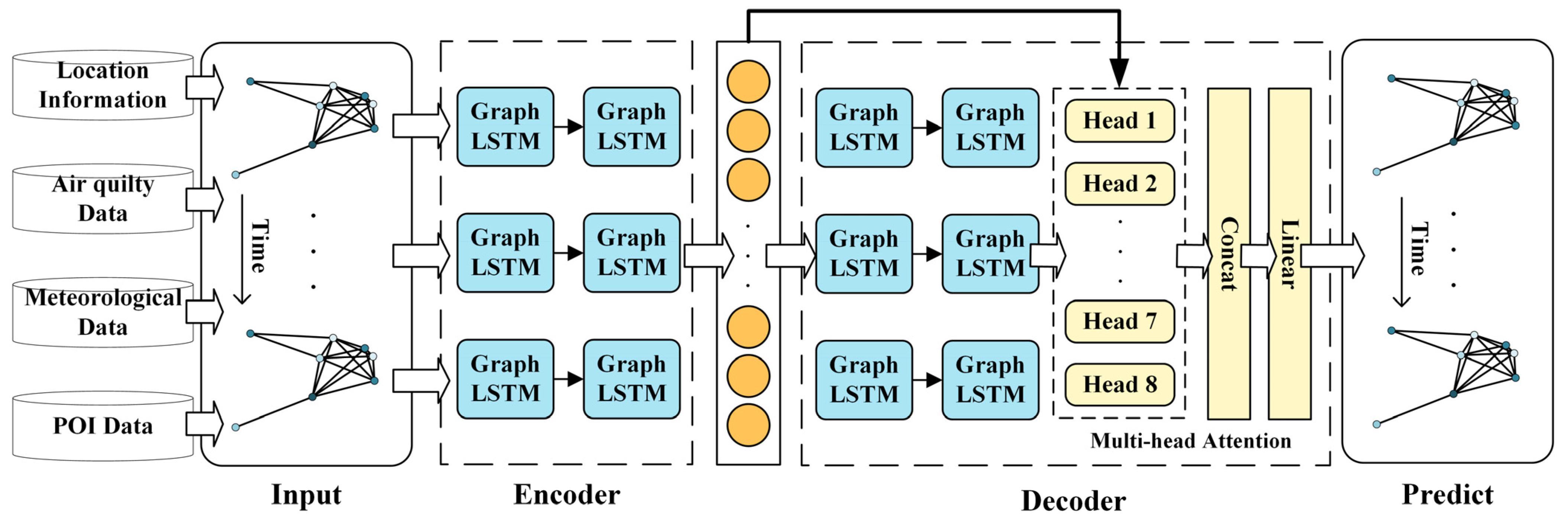
The spatio-temporal prediction of air quality continues to present challenges in aggregating and integrating spatial site information, as well as addressing the issue of information decay in time series models when handling long sequences. This study proposes a GLSTMMA spatio-temporal prediction model for air quality that incorporates a multi-attention mechanism. By establishing a spatial graph structure incorporating air quality data and its associated features, leveraging the capabilities of GCN to acquire feature representations of the site nodes within the graph structure, and utilizing the LSTM network for sequence modeling to capture long-term information in the temporal domain, this study comprehensively addresses the spatial and temporal dependencies inherent in the time series data pertaining to the air quality of the research area. Figure 6 illustrates the detailed architecture of the air quality prediction model, comprising an encoder and a decoder. The encoder is formed by the sequential arrangement of two layers of Graph LSTMs, while the decoder utilizes two layers of Graph LSTM units. To enhance information aggregation capabilities, a multiple-head attention mechanism is integrated into the decoding phase. This mechanism conducts feature extraction from various subspaces to facilitate the effective fusion of spatial representations of the locations and temporal characteristics.
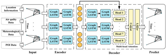
Figure 6.
GLSTMMA architecture.
4.2. Station Relationship Graphs Development
To account for the spatial proximity among sites, this study treats the eight sites as nodes in a graph structure and represents their relationships using an adjacency matrix. If two sites exhibit correlation in the adjacency matrix, it indicates the presence of spatial correlation between these sites and spatial correlation within the monitored data at the site. This study defines a weighted graph to represent the graph structure consisting of eight sites. Here, denotes N sites in the study area; denotes the set of edges; and denotes a neighbor matrix used to represent the spatial relationship weights.
Neighborhood matrix: To accurately represent the spatial distribution characteristics of the site in a non-Euclidean space, it is advisable to develop a graph structure that better aligns with the spatial attributes of the actual problem. The calculation of the geographical position between sites is determined based on their respective latitude and longitude coordinates. In this context, Earth is considered a sphere. Haversine’s equation is employed to address the angular separation between these points, utilizing the sinusoidal function to compute the arc length distance:
where denotes the true distance between site i and site j; denotes the radius of Earth; and denote the latitude and longitude of the site i; and denote the latitude and longitude of site j.
Importing in the Gaussian aggregation function as the weight for the edges connecting the nodes enhances the representation of connectivity between nodes in a linear fashion. This approach aids in the seamless integration of spatial features across different locations within the graph structure. Here, denotes the connectivity between nodes and on the graph, which is calculated as follows:
where denotes the edge weights calculated based on the distances between sites. These weights are instrumental in regulating the distribution and sparsity of the weighted adjacency matrix. The values in the matrix are determined by both the factual distances between the sites and the pre-existing knowledge.
Feature matrix: To comprehensively assess the impacts on air quality at the specific location, a feature matrix is created incorporating air quality data (PM2.5, PM10, NO2, O3, SO2, CO, AQI), meteorological factors (T2M, WD, WS, SP, TP, BLH, RH), and 12 categories of point of interest (POI) data surrounding the site. This matrix is then combined with neighboring matrices to establish a spatio-temporal correlation data framework. The neighbor matrix is utilized for the development of the spatio-temporal correlation data structure. Therefore, is defined as the feature matrices representing the air quality and associated characteristics of the site at different time points within a graph structure.
where M denotes the feature dimension; N denotes the number of stations; and denotes the air quality and related feature data of all stations at time t.
4.3. Temporal Graph Convolutional Modules
GCN: GCN is a model that expands upon CNN to accommodate graph structures. This extension offers a novel approach for capturing spatial features that are unevenly distributed in non-Euclidean spaces. Upon finalizing the development of the adjacency matrix and feature matrix among sites, the specific equation for GCN in the hidden layer is outlined as follows:
where denotes the computation of the hidden layer of the GCN network; denotes the matrix after the addition of the adjacency matrix and the unit matrix (i.e., , is the unit matrices); denotes the degree matrix of (i.e., ); denotes the weight matrix; and denotes the activation function.
LSTM: The LSTM model represents an advancement over the RNN model. In comparison to traditional neural network units, RNN can capture the impact from preceding networks. However, as the chain of information propagation extends to a certain length, the network may encounter issues such as vanishing or exploding gradients. LSTM addresses this challenge by incorporating a Gating Mechanism, which regulates forgetting gates, input gates, and output gates to manage information retention, addition, and output. This mechanism effectively mitigates the long-term dependency problem encountered in simple RNN. The specific information transfer calculations within an LSTM unit are detailed in the following Equations (6)–(10).
Equation (6) derives a forgetting vector by considering the input of the current unit at time t and incorporating the short-term memory information received from the preceding unit after passing through the forgetting gate structure. Subsequently, Equation (7) utilizes the input gate structure to compute an input vector . Equation (8) determines the retention of long-term memory for network propagation and the retention of current candidate information in long-term memory within the network based on and , respectively. Following this, Equation (9) employs the output gate structure to calculate an output vector . Finally, Equation (10) extracts the output information and the short-term memory state of the network from the long-term memory c and the output vector o of the current cell. In Equations (6)–(10), denotes the activation function; , , and denote the hidden layer weights of the forgetting gate, the input gate, and the output gate, respectively; denotes the hidden layer weight matrix of the current candidate state of the computational unit; , , and denote the offset vectors for the three gate structures, respectively; and denotes the offset vector for computing the candidate states.
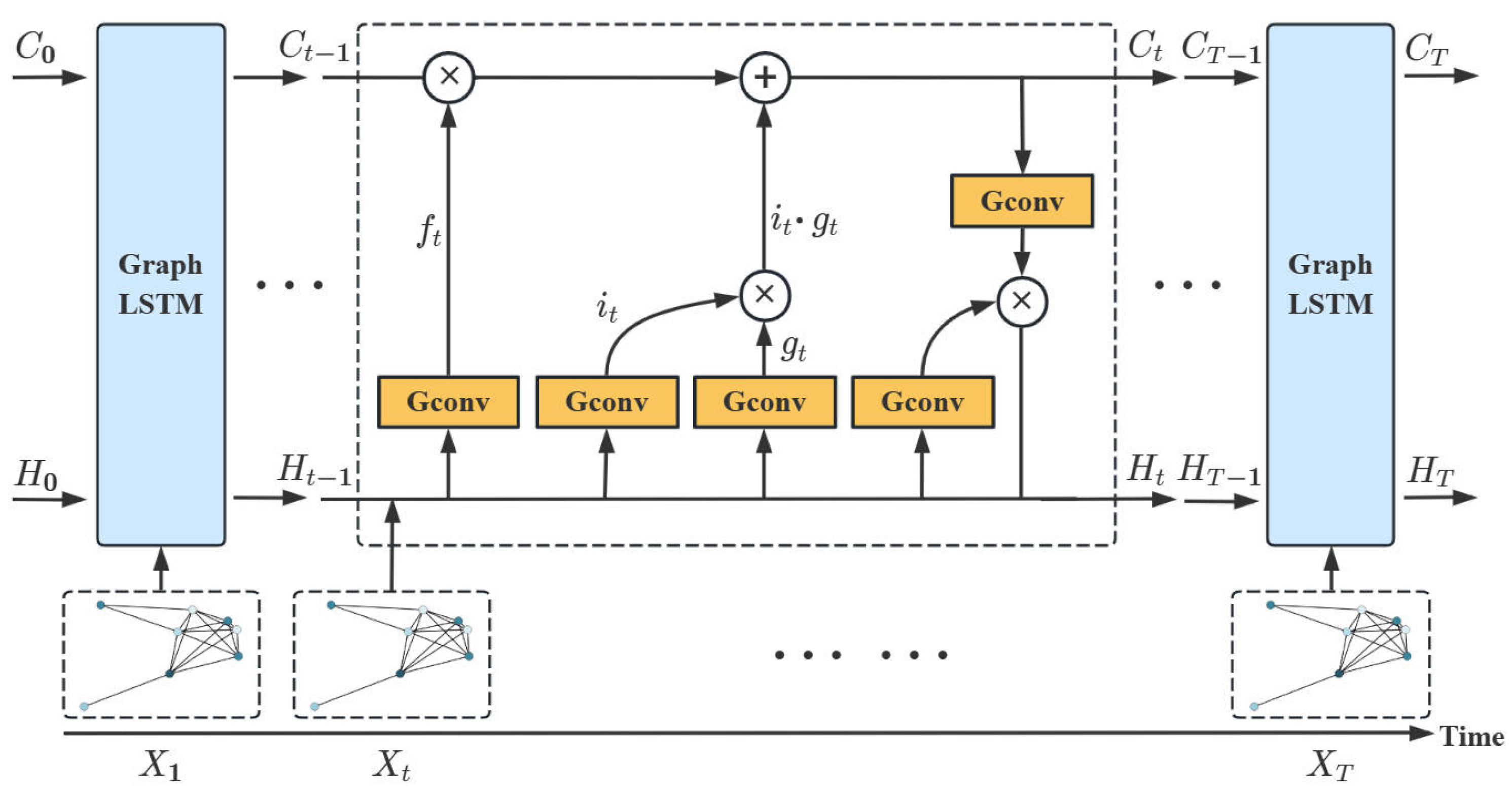
Graph LSTM: The core component of the model proposed in this study comprises GCN and LSTM units. The extraction of the spatial feature of the site is achieved through GCN and subsequently integrated into the graph signal . By employing as an input in the time-dependent model LSTM network, the matrix multiplications in the hidden states of the oblivion gate, input gate, output gate, and candidate gate are substituted with a GCN operator to facilitate a proficient fusion of spatio-temporal features. The network architecture of Graph LSTM is illustrated in Figure 7.

Figure 7.
Graph LSTM architecture.
The recursive unit of Graph LSTM updates the hidden state of all sites based on LSTM, calculated as follows:
where denotes the information after the fusion of spatial features and graph signals at time t; , , and denote the forgetting gate, input gate, and output gate, respectively; and denote the candidate hidden state and hidden state at time t, respectively; and denotes the activation function. Multiple Graph LSTM units are interconnected in a sequential manner, enabling the transmission of spatio-temporal information by passing the hidden state output of each recursive unit as input to the subsequent recursive unit.
4.4. Encoder-Multi-Head Attention Enhanced Decoder
The air quality prediction model achieves end-to-end sequence prediction through the utilization of multiple Graph LSTM layers that are stacked and interconnected to create both an encoder and a decoder. The encoder comprises two Graph LSTM layers that generate the encoding context vector through iterative encoding of the input raw data features in a loop. The decoder comprises two Graph LSTM layers. It utilizes the encoder output vector from the previous time step as the current input, amalgamates the encoder representation, and cyclically decodes the complete target sequence to generate the entire output. Additionally, a multi-head attention mechanism is integrated into the top layer to concentrate specifically on the encoder representation. The integration of multi-head attention enables the decoder to concentrate on contextual semantic information from various viewpoints. Additionally, regularization of its weight distribution to a certain degree helps prevent overfitting of the model, thereby enhancing the efficacy of sequence prediction.
The Query, Key, and Value components of the multi-attention mechanism need to be linearly varied to derive the final Q, K, and V. The computation of the multi-attention mechanism employed in this study is illustrated in Equations (16)–(21).
where the initial state of Query matrix in Equation (16) is a linear transformation of the encoder’s output ; the initial state of Key matrix in Equation (17) is a linear transformation of the encoder’s hidden state ; the initial state of Value matrix in Equation (18) is a linear transformation of the encoder’s hidden state ; and the initial state of Key matrix in Equation (18) is a linear transformation of the encoder’s hidden state . Equation (19) involves the multiplication of and , followed by division by the scaling factor . The result is then processed through the softmax activation function to derive the attention score . Equation (20) calculates the attentional output for each head by multiplying and . Equation (21) combines the attention scores from all heads to generate the attention output .
The model is developed by sequentially stacking Graph LSTM units to create an encoder for feature extraction and a decoder for temporal prediction. The encoder and decoder collaborate to integrate attention mechanisms, improving the contextual semantic representation and maintaining spatio-temporal relevance in the modeling process. The architecture is designed to enhance the model’s performance in predicting sequences of air quality changes.
5. Results and Discussion
5.1. Experimental Setup
The experimental setup includes the configuration of hardware and software environments and related parameters. This study builds deep learning models based on the Pytorch framework. All tests of the experiment use 24 h as a historical time window for predicting the air pollutant observations in 1, 3, 6, 12, and 24 h (H = 1, 3, 6, 12, 24) of observed air pollutant values. The search for the model’s optimal hyperparameters was automated using a grid search method with set ranges of values and step sizes for the parameters. The model uses an Adma optimizer with a mean square error (MSE) loss function to update the parameters, setting the initial value of the learning rate to 0.01 and adjusting it dynamically, epoch to 100, and batch-size to 256.
The model involves utilizing hourly-level air quality observations spanning from 2019 to 2021. The data are partitioned such that the initial 70% is allocated for training the model, 10% for validation, and the remaining 20% for assessing prediction performance. Mean absolute error (MAE), mean absolute percentage error (MAPE), and root mean square error (RMSE) metrics have been chosen to evaluate the predictive accuracy of the GLSTMMA model in comparison to other baseline models. These metrics are expressed as follows:
where denotes the observed true value and denotes the predicted value.
Meanwhile, the predictive efficacy of the proposed GLSTMMA model is contrasted with the baseline model for comparison.
Static refers to utilizing the previous moment’s observation as the basis for predicting the current moment.
Historical average (HA) refers to the method that computes the arithmetic mean of past observations and employs it as a forecast. This method presupposes that the time series exhibits smoothness and that forthcoming values are equivalent to HA.
The Vector autoregressive (VAR) model is a generalized autoregressive moving average model. VAR assumes that each time series variable is a linear function of the other time series variables. It predicts its own value by incorporating its lagged values as well as the lagged values of the other variables.
LSTM is a type of temporal neural network designed to manage the retention and discarding of past information by utilizing mechanisms like forgetting gates and input gates. It is specifically tailored for modeling long-term dependencies in time series data.
GRU is a type of RNN characterized by a simplified structure featuring only two control gates. It is designed to effectively manage historical information through mechanisms of saving and forgetting, while also demonstrating proficiency in modeling long sequences similar to an LSTM.
The CNN-LSTM network [49] integrates convolutional operations into the cyclic state transfer mechanism. In contrast to conventional RNN models, CNN-LSTM has the capability to capture spatial characteristics of data and integrate both spatial and temporal information to enhance predictive performance.
5.2. Experimental Results
Table 4 and Table 5 demonstrate the quantitative results of the air quality dataset in Qinghai Province regarding the forecasting of six air pollutants (PM2.5, PM10, NO2, O3, SO2, and CO) at 3, 6, 12, and 24 multi-step time intervals. Among these metrics, MAE, RMSE, and MAPE were comparatively evaluated across various models including Static, HA, VAR, LSTM, GRU, and CNN-LSTM. Additionally, MAE, RMSE, and MAPE of the proposed GLSTMMA model were also assessed in this study. As demonstrated in Table 4 and Table 5, the GLSTMMA model exhibits superior prediction performance at 3, 6, 12, and 24 h in comparison to the other baseline models. The model exhibits MAEs of 4.48, 5.13, 5.77, and 6.24 when predicting PM2.5 at 3, 6, 12, and 24 time steps, respectively. For PM10 prediction, the model shows MAEs of 9.96, 11.34, 12.44, and 13.42 at 3, 6, 12, and 24 time steps, respectively. Similarly, in the case of O3 prediction, the model demonstrates MAEs of 9.96, 11.34, 12.44, and 13.42 at 3, 6, 12, and 24 time steps, respectively. When predicting NO2 levels, the model achieved MAEs of 5.21, 5.72, 6.19, and 6.49 at 3, 6, 12, and 24 time steps, respectively. For SO2 predictions, the model’s MAE values at the same time steps were 2.74, 3.13, 3.55, and 3.94, respectively. In the prediction of CO levels, MAEs of the model at 3, 6, 12, and 24 time steps were 0.12, 0.13, 0.15, and 0.16, respectively. The results indicate that the GLSTMMA model exhibited the lowest prediction error and the highest prediction accuracy. When using the HA model for forecasting, for each time step, predictions are made based on the historical average values from the corresponding past time period, and the method of processing historical data is fixed. Therefore, the forecasting results do not change with variations in the time step. Furthermore, classical deep learning models such as LSTM and GRU exhibit modeling errors that are comparatively lower than those of statistical models. The limited quantity and uneven spatial distribution of stations within the study area resulted in poor stabilization of the CNN-LSTM model during the prediction process, leading to prediction errors that were once again lower compared to those of the statistical model. This implies that deep learning models may outperform traditional statistical learning models in predicting air quality time series across multiple time steps.
Table 4.
Comparison error analysis of GLSTMMA and other baseline models for PM2.5, PM10, and O3 prediction.
Table 5.
Comparison error analysis of GLSTMMA and other baseline models for NO2, SO2, and CO prediction.
The predictive performance of the GLSTMMA model at different time steps was explored using the relative root mean square error (rRMSE = RMSE/RMSEbaseline) compared to the baseline model (HA). The specific results are presented in Table 4 and Table 5. A gradual decrease in model prediction performance was observed as the time step increased. This underscores the importance of improving the accuracy of long time series predictions. Consequently, future research should focus on enhancing the model’s precision in predicting long time series data.
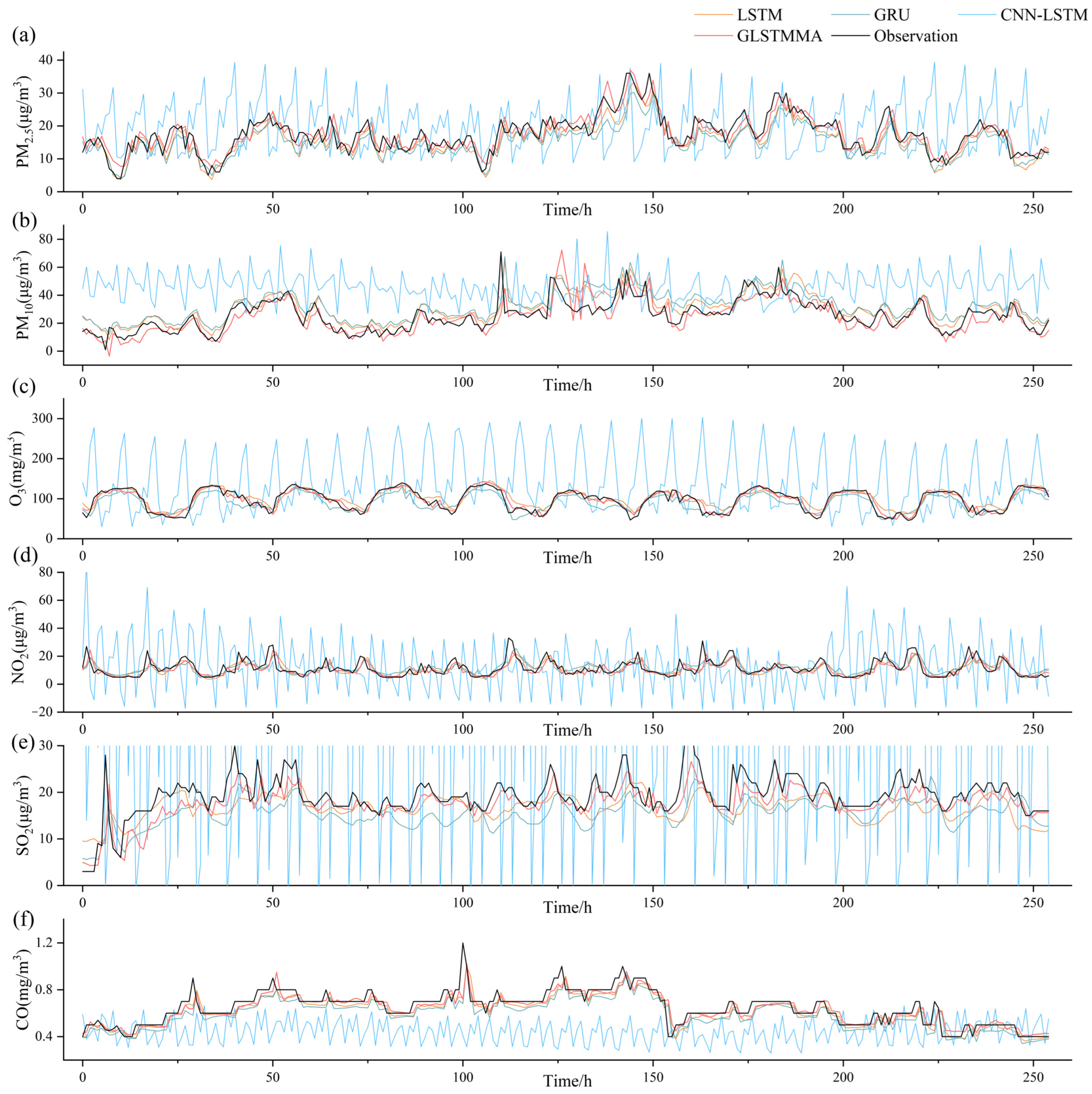
To facilitate a more intuitive analysis and comparison of the disparities between the prediction outcomes and the actual values of the GLSTMMA model, see Figure 8. The prediction results and true observed values of the six pollutants using the GLSTMMA model for 24 time steps are illustrated in Figure 8a–f. The x-coordinate represents the observation time, while the y-coordinate represents the concentration value of the pollutant. Based on the results, the model demonstrates a higher accuracy in forecasting the future hourly trends of the six pollutants. The variance between the predicted values and actual measurements is minimal. However, the model’s efficacy diminishes when anticipating peak pollutant concentrations.
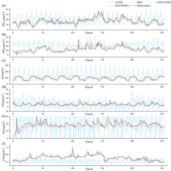
Figure 8.
Comparison of model predictions versus true values. (a–f) represent comparisons of model-predicted PM2.5, PM10, O3, NO2, SO2, and CO concentrations with their respective true values, respectively.
5.3. Model Effectiveness Evaluation
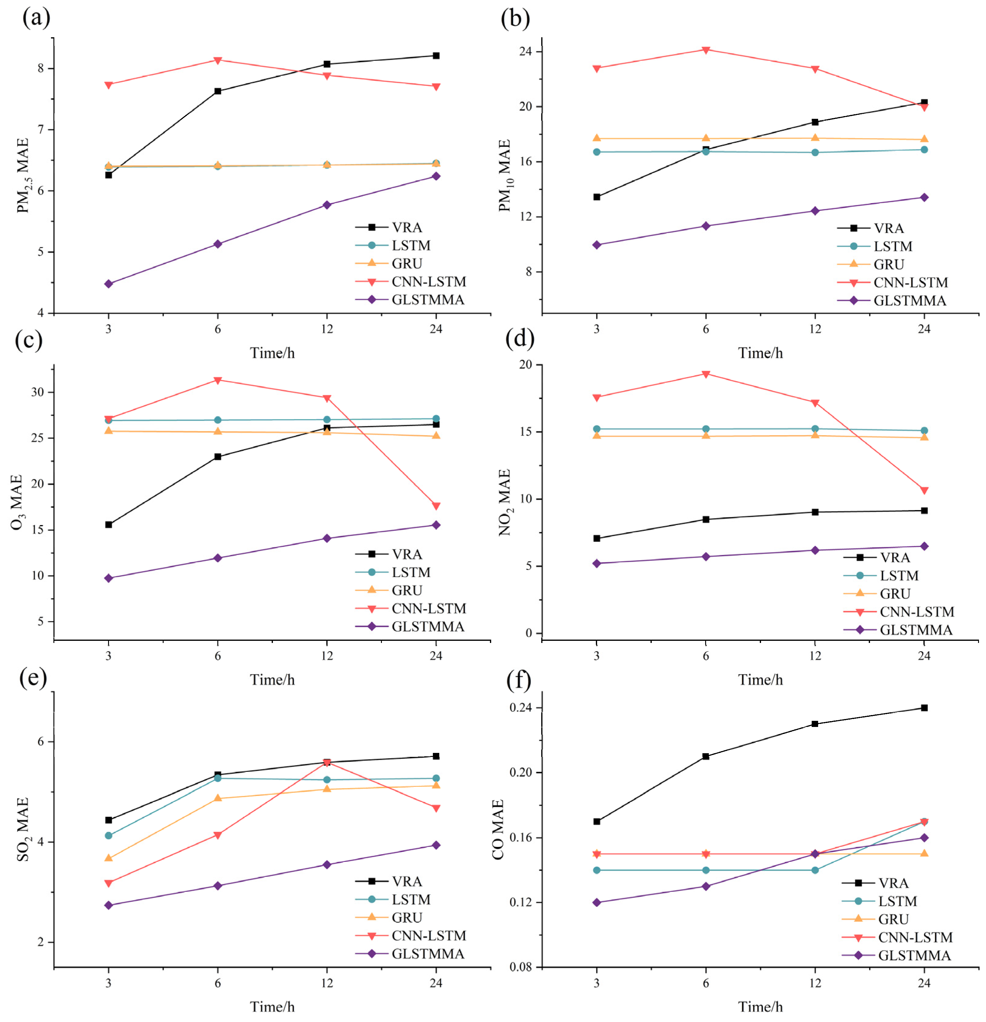
Given that MAE can provide a more accurate representation of prediction value errors, this study visualized the curves of prediction step size versus MAE to illustrate this relationship. The comparative outcomes of the variation curves depicting the prediction step size against MAE for six air pollutants utilizing various models such as VAR, LSTM, GRU, CNN-LSTM, and GLSTMMA are represented in Figure 9.
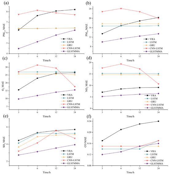
Figure 9.
Comparative analysis of MAE across prediction step sizes for VAR, LSTM, GRU, CNN-LSTM, and GLSTMMA models. (a–f) represent the comparison results for PM2.5, PM10, O3, NO2, SO2, and CO, respectively.
Based on the results (Figure 8), the GLSTMMA model exhibits superior predictive performance in comparison to the VAR, LSTM, GRU, and CNN-LSTM models across all air pollutants. Furthermore, the prediction errors of the VRA and GLSTMMA models exhibit a gradual and smooth increase as the step size increases. Conversely, the LSTM and GRU models demonstrate a more moderate change with a slight decreasing trend across various prediction steps. The CNN-LSTM model’s predictions display greater instability, showing varying performances across different prediction objects and steps. This variability may be attributed to the limited number and sparse distribution of study sites. The challenges in learning the characteristics of unevenly distributed site changes with CNN further support the notion that GCN is more effective in scenarios with sparse sites.
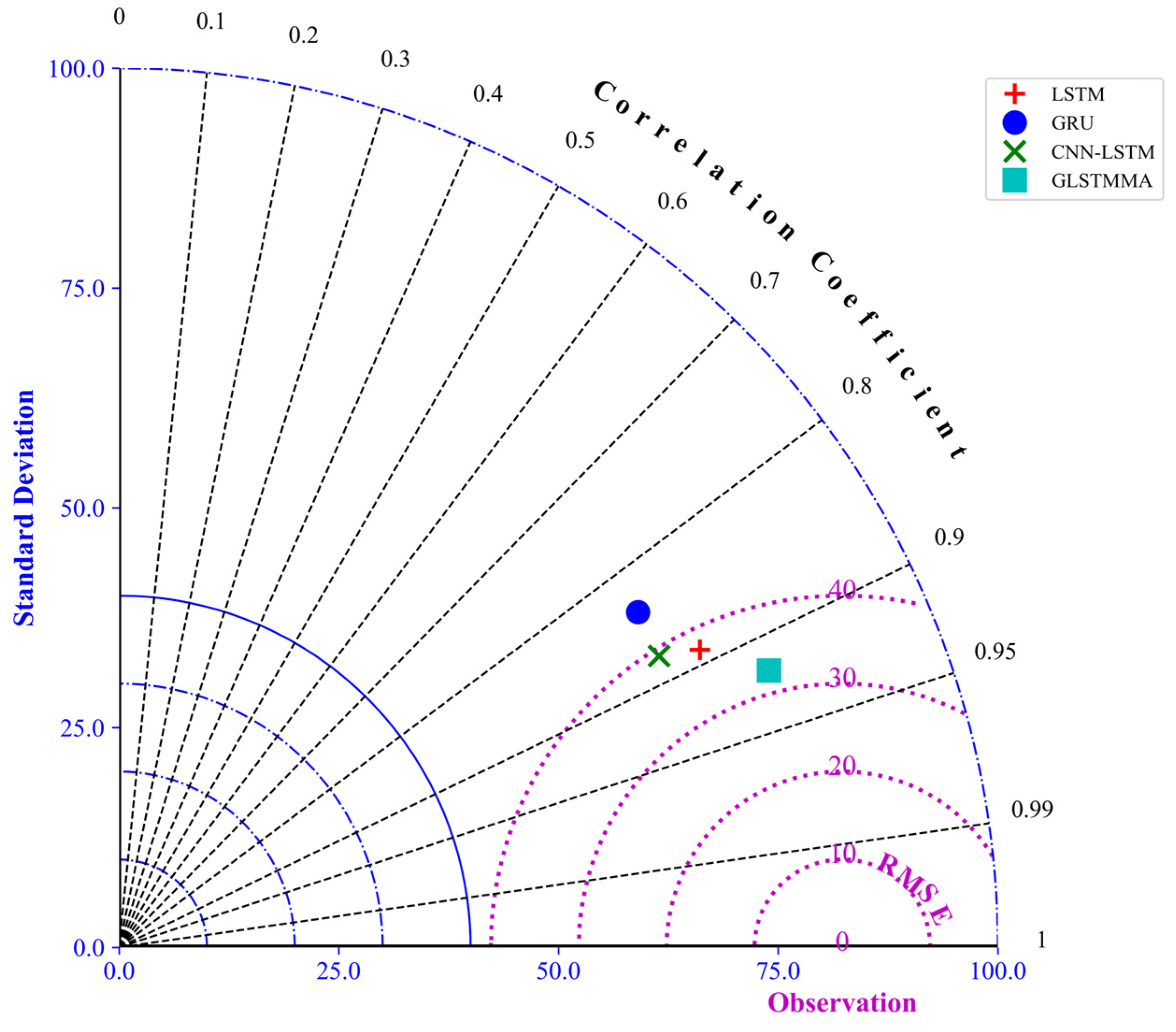
By plotting a Taylor diagram to comprehensively consider three key indicators—standard deviation, correlation coefficient, and RMSE—the performance of four models, namely LSTM, GRU, CNN-LSTM, and GLSTMMA, was compared in predicting ozone concentration. As observed in Figure 10, the GLSTMMA model excels in all three indicators, with its point closest to the origin of the observed values. This indicates that GLSTMMA not only exhibits a high correlation with the actual observed values when predicting ozone concentration but also has the smallest standard deviation and RMSE of its predictions, thus achieving the highest prediction accuracy. LSTM shows relatively small prediction errors, lower standard deviation, lower RMSE, and a higher correlation coefficient. On the other hand, GRU and CNN-LSTM exhibit relatively large prediction errors, higher standard deviation, higher RMSE, and a lower correlation coefficient. In summary, this study validates the superiority of the GLSTMMA model in predicting ozone concentration, providing a valuable reference for developing more accurate air quality forecasting models. The differences among the different models in various evaluation indicators suggest that combining the advantages of multiple models may further improve prediction accuracy, which is a direction for future research to explore.

Figure 10.
Correlation analysis of different deep learning models in O3 concentration prediction.
The superior predictive performance of the GLSTMMA model can be attributed to several key factors. Firstly, the gradual and smooth increase in prediction errors with increasing step size indicates the model’s robustness and stability in handling varying prediction intervals. This contrasts with other models like VRA, LSTM, GRU, and CNN-LSTM, which show more pronounced fluctuations in prediction errors, suggesting that GLSTMMA maintains better consistency across different prediction steps. Secondly, the GLSTMMA model’s ability to excel in all three key indicators—standard deviation, correlation coefficient, and RMSE—demonstrates its overall accuracy, precision, and reliability in predicting pollutant concentration compared to other models. These combined advantages make GLSTMMA a standout choice for predicting pollutant concentration and provide valuable insights for developing more accurate and reliable air quality forecasting models in the future.
5.4. Dataset Validity Analysis
Controlled experiments were intentionally designed in this study to assess the efficacy of air quality datasets that integrate multi-source data in enhancing the accuracy of air quality predictions. Prediction experiments were conducted for six major air pollutants using the GLSTMMA model. The experiments considered the control variables method and utilized datasets solely containing air quality data, without incorporating any other auxiliary data. The prediction outcomes of the two datasets on the GLSTMMA model are presented in Table 6.
Table 6.
Comparison of air quality prediction results for different datasets.
In Table 6, MAE, RMSE, and MAPE metrics for predicting the six air pollutants show varying degrees of improvement when solely using the air quality data compared to the comprehensive dataset that integrates data from multiple sources. The significance of the multi-source air quality dataset in enhancing the prediction model is illustrated in Figure 11. Upon the integration of the multi-source data, the correlation among the data sets enriches the features available for the model. This enrichment facilitates the exploration of the intricate relationships within the data, consequently enhancing the accuracy of the prediction. Therefore, the outcomes of the controlled experiments unequivocally confirm the efficacy of integrating air quality datasets with data from multiple sources. When air quality data are integrated with other pertinent meteorological, environmental, and social data, the predictive accuracy of air quality can be substantially enhanced through the utilization of deep learning models.
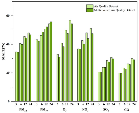
Figure 11.
Comparison of predictions for different datasets.
For future studies and practical applications, constructing air quality prediction datasets should focus on integrating diverse data sources beyond traditional air quality measurements. Incorporating meteorological parameters such as temperature, humidity, wind speed, and direction can provide valuable insights into atmospheric dynamics that influence air quality. Additionally, including environmental factors like land use, vegetation cover, and emission sources such as industrial activities and vehicular traffic can offer a more comprehensive understanding of air quality variations. Moreover, integrating social data such as population density, traffic patterns, and urban development can help capture the human impact on air quality. By amalgamating these multi-source datasets, future prediction models can leverage a richer set of features, thereby improving the accuracy and reliability of air quality forecasts.
6. Conclusions
In this study, a novel air quality forecasting model employing a hybrid deep learning methodology is introduced to enable the 24 h prediction of six air pollutants, specifically PM2.5, PM10, NO2, O3, SO2, and CO. The fundamental component of the GLSTMMA model consists of a Graph LSTM that integrates a hybrid GCN and LSTM neural network. The encoder comprises a two-layer Graph LSTM, while the decoder is a two-layer Graph LSTM augmented by a multi-head attention mechanism. The model is capable of acquiring time series data on air quality along with associated information such as meteorological conditions and POI, as well as the relevant features concerning the spatio-temporal dependence of air quality. Experiments conducted on the air quality dataset of Qinghai Province, China (2019–2021) demonstrate that the model exhibits enhanced performance in comparison to conventional statistical models and traditional deep learning prediction models. This improvement is attributed to its ability to analyze the learning of multivariate dependencies within air quality-related time series and spatial correlations. It is significant to explore the evolution of air pollutant time series in future research endeavors to advance the study and enhancement of the GLSTMMA model under varying prediction scenarios.
Author Contributions
Conceptualization, Y.W., K.L., and Y.H.; methodology, Y.W. and K.L.; software, Y.H.; validation, Y.W., P.W., and Y.C.; formal analysis, H.X.; investigation, C.H.; resources, Y.W.; data curation, L.L.; writing—original draft preparation, Y.W.; writing—review and editing, Y.W. and P.W.; visualization, Y.W.; supervision, Y.W.; project administration, Y.W.; funding acquisition, Y.W. All authors have read and agreed to the published version of the manuscript.
Funding
This research was funded by the North China Institute of Aerospace Engineering Doctoral Fund: Research on Spatio-Temporal Data Fusion Analysis of Beijing–Tianjin–Hebei City Cluster (Grant No. BKY-2020-33) and the Qinghai Province Air Pollution Status Assessment and Refined Management Support Project (Grant No. 2023-005).
Institutional Review Board Statement
Not applicable.
Informed Consent Statement
Not applicable.
Data Availability Statement
Air quality data published by the China National Environmental Monitoring Centre: https://quotsoft.net/air/, retrieved on 22 January 2023.
Conflicts of Interest
The authors declare no conflicts of interest.
References
- Manisalidis, I.; Stavropoulou, E.; Stavropoulos, A.; Bezirtzoglou, E. Environmental and health impacts of air pollution: A review. Front. Public Health 2020, 8, 14. [Google Scholar] [CrossRef] [PubMed]
- Shaddick, G.; Thomas, M.L.; Mudu, P.; Ruggeri, G.; Gumy, S. Half the world’s population are exposed to increasing air pollution. npj Clim. Atmos. Sci. 2020, 3, 23. [Google Scholar] [CrossRef]
- Kang, G.K.; Gao, J.Z.; Chiao, S.; Lu, S.; Xie, G. Air quality prediction: Big data and machine learning approaches. Int. J. Environ. Sci. Dev. 2018, 9, 8–16. [Google Scholar] [CrossRef]
- Kampa, M.; Castanas, E. Human health effects of air pollution. Environ. Pollut. 2008, 151, 362–367. [Google Scholar] [CrossRef]
- Glencross, D.A.; Ho, T.-R.; Camina, N.; Hawrylowicz, C.M.; Pfeffer, P.E. Air pollution and its effects on the immune system. Free Radic. Biol. Med. 2020, 151, 56–68. [Google Scholar] [CrossRef]
- Sarkheil, H.; Rahbari, S. Development of case historical logical air quality indices via fuzzy mathematics (Mamdani and Takagi–Sugeno systems), a case study for Shahre Rey Town. Environ. Earth Sci. 2016, 75, 1319. [Google Scholar] [CrossRef]
- Lu, J.G. Air pollution: A systematic review of its psychological, economic, and social effects. Curr. Opin. Psychol. 2020, 32, 52–65. [Google Scholar] [CrossRef]
- Tainio, M.; Andersen, Z.J.; Nieuwenhuijsen, M.J.; Hu, L.; De Nazelle, A.; An, R.; Garcia, L.M.; Goenka, S.; Zapata-Diomedi, B.; Bull, F.; et al. Air pollution, physical activity and health: A mapping review of the evidence. Environ. Int. 2021, 147, 105954. [Google Scholar] [CrossRef] [PubMed]
- Alahmad, B.; Khraishah, H.; Althalji, K.; Borchert, W.; Al-Mulla, F.; Koutrakis, P. Connections between air pollution, climate change, and cardiovascular health. Can. J. Cardiol. 2023, 39, 1182–1190. [Google Scholar] [CrossRef]
- Lu, X.; Zhang, S.; Xing, J.; Wang, Y.; Chen, W.; Ding, D.; Wu, Y.; Wang, S.; Duan, L.; Hao, J. Progress of air pollution control in China and its challenges and opportunities in the ecological civilization era. Engineering 2020, 6, 1423–1431. [Google Scholar] [CrossRef]
- Cabaneros, S.M.; Calautit, J.K.; Hughes, B.R. A review of artificial neural network models for ambient air pollution prediction. Environ. Model. Softw. 2019, 119, 285–304. [Google Scholar] [CrossRef]
- Gonzalez-Martin, J.; Kraakman, N.J.R.; Perez, C.; Lebrero, R.; Munoz, R. A state–of–the-art review on indoor air pollution and strategies for indoor air pollution control. Chemosphere 2021, 262, 128376. [Google Scholar] [CrossRef]
- Zhao, H.; Chen, K.; Liu, Z.; Zhang, Y.; Shao, T.; Zhang, H. Coordinated control of PM2. 5 and O3 is urgently needed in China after implementation of the “Air pollution prevention and control action plan”. Chemosphere 2021, 270, 129441. [Google Scholar] [CrossRef] [PubMed]
- Chu, Z.; Bian, C.; Yang, J. Joint prevention and control mechanism for air pollution regulations in China: A policy simulation approach with evolutionary game. Environ. Impact Assess. Rev. 2021, 91, 106668. [Google Scholar] [CrossRef]
- Yang, X.; Wu, H.; Ren, S.; Ran, Q.; Zhang, J. Does the development of the internet contribute to air pollution control in China? Mechanism discussion and empirical test. Struct. Chang. Econ. Dyn. 2021, 56, 207–224. [Google Scholar] [CrossRef]
- Ma, J.; Cheng, J.C.; Lin, C.; Tan, Y.; Zhang, J. Improving air quality prediction accuracy at larger temporal resolutions using deep learning and transfer learning techniques. Atmos. Environ. 2019, 214, 116885. [Google Scholar] [CrossRef]
- Ameer, S.; Shah, M.A.; Khan, A.; Song, H.; Maple, C.; Islam, S.U.; Asghar, M.N. Comparative analysis of machine learning techniques for predicting air quality in smart cities. IEEE Access 2019, 7, 128325–128338. [Google Scholar] [CrossRef]
- Iskandaryan, D.; Ramos, F.; Trilles, S.J. Air quality prediction in smart cities using machine learning technologies based on sensor data: A review. Appl. Sci. 2020, 10, 2401. [Google Scholar] [CrossRef]
- Masood, A.; Ahmad, K.J. A review on emerging artificial intelligence (AI) techniques for air pollution forecasting: Fundamentals, application and performance. J. Clean. Prod. 2021, 322, 129072. [Google Scholar] [CrossRef]
- Mitreska Jovanovska, E.; Batz, V.; Lameski, P.; Zdravevski, E.; Herzog, M.A.; Trajkovik, V. Methods for urban Air Pollution measurement and forecasting: Challenges, opportunities, and solutions. Atmosphere 2023, 14, 1441. [Google Scholar] [CrossRef]
- Liao, Q.; Zhu, M.; Wu, L.; Pan, X.; Tang, X.; Wang, Z. Deep learning for air quality forecasts: A review. Curr. Pollut. Rep. 2020, 6, 399–409. [Google Scholar] [CrossRef]
- Hanna, S.R.; Egan, B.A.; Purdum, J.; Wagler, J. Evaluation of the ADMS, AERMOD, and ISC3 dispersion models with the OPTEX, Duke Forest, Kincaid, Indianapolis and Lovett field datasets. Int. J. Environ. Pollut. 2001, 16, 301–314. [Google Scholar] [CrossRef]
- Moore, G.E.; Londergan, R.J. Sampled Monte Carlo uncertainty analysis for photochemical grid models. Atmos. Environ. 2001, 35, 4863–4876. [Google Scholar] [CrossRef]
- Levy, J.I.; Spengler, J.D.; Hlinka, D.; Sullivan, D.; Moon, D. Using CALPUFF to evaluate the impacts of power plant emissions in Illinois: Model sensitivity and implications. Atmos. Environ. 2002, 36, 1063–1075. [Google Scholar] [CrossRef]
- Makar, P.; Stockwell, W.; Li, S. Gas-phase chemical mechanism compression strategies: Treatment of reactants. Atmos. Environ. 1996, 30, 831–842. [Google Scholar] [CrossRef]
- Byun, D.; Schere, K.L. Review of the governing equations, computational algorithms, and other components of the Models-3 Community Multiscale Air Quality (CMAQ) modeling system. Appl. Mech. Rev. 2006, 59, 51–77. [Google Scholar] [CrossRef]
- Wang, Z.; Itahashi, S.; Uno, I.; Pan, X.; Osada, K.; Yamamoto, S.; Nishizawa, T.; Tamura, K.; Wang, Z. Modeling the long-range transport of particulate matters for January in East Asia using NAQPMS and CMAQ. Aerosol Air Qual. Res. 2017, 17, 3065–3078. [Google Scholar] [CrossRef]
- Stockwell, W.R.; Lawson, C.V.; Saunders, E.; Goliff, W.S. A review of tropospheric atmospheric chemistry and gas-phase chemical mechanisms for air quality modeling. Atmosphere 2011, 3, 1–32. [Google Scholar] [CrossRef]
- Liao, K.; Huang, X.; Dang, H.; Ren, Y.; Zuo, S.; Duan, C. Statistical approaches for forecasting primary air pollutants: A review. Atmosphere 2021, 12, 686. [Google Scholar] [CrossRef]
- Wang, J.; Ji, H.; Wang, Q.g.; Li, H.; Qian, X.; Li, F.; Yang, M. Prediction of size-fractionated airborne particle-bound metals using MLR, BP-ANN and SVM analyses. Chemosphere 2017, 180, 513–522. [Google Scholar]
- Abhilash, M.; Thakur, A.; Gupta, D.; Sreevidya, B. Time series analysis of air pollution in Bengaluru using ARIMA model. In Ambient Communications and Computer Systems: RACCCS 2017; Springer: Singapore, 2018; pp. 413–426. [Google Scholar]
- Rybarczyk, Y.; Zalakeviciute, R. Machine learning approaches for outdoor air quality modelling: A systematic review. Appl. Sci. 2018, 8, 2570. [Google Scholar] [CrossRef]
- Ayturan, Y.A.; Ayturan, Z.C.; Altun, H.O. Air pollution modelling with deep learning: A review. Int. J. Environ. Pollut. Environ. Model. 2018, 1, 58–62. [Google Scholar]
- Zhang, B.; Rong, Y.; Yong, R.; Qin, D.; Li, M.; Zou, G.; Pan, J. Deep learning for air pollutant concentration prediction: A review. Atmos. Environ. 2022, 290, 119347. [Google Scholar] [CrossRef]
- LeCun, Y.; Bengio, Y.; Hinton, G. Deep learning. Nature 2015, 521, 436–444. [Google Scholar] [CrossRef] [PubMed]
- Athira, V.; Geetha, P.; Vinayakumar, R.; Soman, K. Deepairnet: Applying recurrent networks for air quality prediction. Procedia Comput. Sci. 2018, 132, 1394–1403. [Google Scholar]
- Seng, D.; Zhang, Q.; Zhang, X.; Chen, G.; Chen, X. Spatiotemporal prediction of air quality based on LSTM neural network. Alex. Eng. J. 2021, 60, 2021–2032. [Google Scholar] [CrossRef]
- Wang, X.; Yan, J.; Wang, X.; Wang, Y. Air quality forecasting using GRU model based on multiple sensors nodes. IEEE Sens. Lett. 2023, 7, 6003804. [Google Scholar] [CrossRef]
- Wang, J.; Li, X.; Jin, L.; Li, J.; Sun, Q.; Wang, H. An air quality index prediction model based on CNN-ILSTM. Sci. Rep. 2022, 12, 8373. [Google Scholar] [CrossRef]
- Ge, L.; Wu, K.; Zeng, Y.; Chang, F.; Wang, Y.; Li, S. Multi-scale spatiotemporal graph convolution network for air quality prediction. Appl. Intell. 2021, 51, 3491–3505. [Google Scholar] [CrossRef]
- El-Harbawi, M. Air quality modelling, simulation, and computational methods: A review. Environ. Rev. 2013, 21, 149–179. [Google Scholar] [CrossRef]
- Dennis, R.L.; Arnold, J.; Tonnesen, G.S.; Li, Y. A new response surface approach for interpreting Eulerian air quality model sensitivities. Comput. Phys. Commun. 1999, 117, 99–112. [Google Scholar] [CrossRef]
- Hu, J.; Chen, J.; Ying, Q.; Zhang, H. One-year simulation of ozone and particulate matter in China using WRF/CMAQ modeling system. Atmos. Meas. Tech. 2016, 16, 10333–10350. [Google Scholar] [CrossRef]
- Lei, M.T.; Monjardino, J.; Mendes, L.; Gonçalves, D.; Ferreira, F. Macao air quality forecast using statistical methods. Air Qual. Atmos. Heal. 2019, 12, 1049–1057. [Google Scholar] [CrossRef]
- Kumar, T.S.; Das, H.S.; Choudhary, U.; Dutta, P.E.; Guha, D.; Laskar, Y. Analysis and prediction of air pollution in Assam using ARIMA/SARIMA and machine learning. In Innovations in Sustainable Energy and Technology: Proceedings of ISET 2020; Springer: Singapore, 2021; pp. 317–330. [Google Scholar]
- Liu, W.; Chen, F.; Chen, Y. PM2.5 Concentration Prediction Based on Pollutant Pattern Recognition Using PCA-clustering Method and CS Algorithm Optimized SVR. Nat. Environ. Pollut. Technol. 2022, 21, 393–403. [Google Scholar] [CrossRef]
- Krishan, M.; Jha, S.; Das, J.; Singh, A.; Goyal, M.K.; Sekar, C. Air quality modelling using long short-term memory (LSTM) over NCT-Delhi, India. Air Qual. Atmos. Heal. 2019, 12, 899–908. [Google Scholar] [CrossRef]
- Li, X.; Peng, L.; Hu, Y.; Shao, J.; Chi, T. Deep learning architecture for air quality predictions. Environ. Sci. Pollut. Res. 2016, 23, 22408–22417. [Google Scholar] [CrossRef]
- Yan, R.; Liao, J.; Yang, J.; Sun, W.; Nong, M.; Li, F. Multi-hour and multi-site air quality index forecasting in Beijing using CNN, LSTM, CNN-LSTM, and spatiotemporal clustering. Expert Syst. Appl. 2021, 169, 114513. [Google Scholar] [CrossRef]
- Chen, L.; Xu, J.; Wu, B.; Huang, J. Group-aware graph neural network for nationwide city air quality forecasting. ACM Trans. Knowl. Discov. Data 2023, 18, 1–20. [Google Scholar] [CrossRef]
- Wang, C.; Zhu, Y.; Zang, T.; Liu, H.; Yu, J. Modeling inter-station relationships with attentive temporal graph convolutional network for air quality prediction. In Proceedings of the 14th ACM International Conference on Web Search and Data Mining, Virtual, 8–12 March 2021; pp. 616–634. [Google Scholar]
- Zhao, G.; He, H.; Huang, Y.; Ren, J. Near-surface PM2.5 prediction combining the complex network characterization and graph convolution neural network. Neural Comput. Appl. 2021, 33, 17081–17101. [Google Scholar] [CrossRef]
- Jin, X.-B.; Wang, Z.-Y.; Kong, J.-L.; Bai, Y.-T.; Su, T.-L.; Ma, H.-J.; Chakrabarti, P. Deep spatio-temporal graph network with self-optimization for air quality prediction. Entropy 2023, 25, 247. [Google Scholar] [CrossRef]
- Tang, X.; Wu, N.; Pan, Y. Prediction of Particulate Matter 2.5 Concentration Using a Deep Learning Model with Time-Frequency Domain Information. Appl. Sci. 2023, 13, 12794. [Google Scholar] [CrossRef]
- Ding, H.; Noh, G. A Hybrid Model for Spatiotemporal Air Quality Prediction Based on Interpretable Neural Networks and a Graph Neural Network. Atmosphere 2023, 14, 1807. [Google Scholar] [CrossRef]
- Hu, Y.; Cao, N.; Guo, W.; Chen, M.; Rong, Y.; Lu, H. FedDeep: A Federated Deep Learning Network for Edge Assisted Multi-Urban PM 2.5 Forecasting. Appl. Sci. 2024, 14, 1979. [Google Scholar] [CrossRef]
- Wang, Y.; Liu, K.; He, Y.; Fu, Q.; Luo, W.; Li, W.; Liu, X.; Wang, P.; Xiao, S. Research on Missing Value Imputation to Improve the Validity of Air Quality Data Evaluation on the Qinghai-Tibetan Plateau. Atmosphere 2023, 14, 1821. [Google Scholar] [CrossRef]
- Sarkheil, H.; Fakhari, M.; Rayegani, B.; Bodagh Jamali, J. Reliability assessment in spatial modeling for identification of air pollution (NO2 & CO) probability in Tehran metropolis. Environ. Sci. 2020, 18, 187–202. [Google Scholar]
- Hussain, A.J.; Sankar, T.K.; Vithanage, M.; Ambade, B.; Gautam, S. Black carbon emissions from traffic contribute sustainability to air pollution in urban cities of India. Water Air Soil Pollut. 2023, 234, 217. [Google Scholar] [CrossRef]
- Ambade, B.; Sankar, T.K.; Kumar, A.; Sethi, S.S. Characterization of PAHs and n-alkanes in atmospheric aerosol of Jamshedpur City, India. J. Hazard. Toxic Radioact. Waste 2020, 24, 04020003. [Google Scholar] [CrossRef]
- Ambade, B.; Kumar, A.; Latif, M. Emission sources, Characteristics and risk assessment of particulate bound Polycyclic Aromatic Hydrocarbons (PAHs) from traffic sites. Res. Sq. 2021. [Google Scholar] [CrossRef]


Disclaimer/Publisher’s Note: The statements, opinions and data contained in all publications are solely those of the individual author(s) and contributor(s) and not of MDPI and/or the editor(s). MDPI and/or the editor(s) disclaim responsibility for any injury to people or property resulting from any ideas, methods, instructions or products referred to in the content. |
© 2024 by the authors. Licensee MDPI, Basel, Switzerland. This article is an open access article distributed under the terms and conditions of the Creative Commons Attribution (CC BY) license (https://creativecommons.org/licenses/by/4.0/).