Abstract
Particular matter (PM) constitutes one of the major air pollutants. Human exposure to fine PM (PM with a median diameter less than or equal to 2.5 μm, PM2.5) has many negative and diverse outcomes for human health, such as respiratory mortality, lung cancer, etc. Accurate air-quality forecasting on a regional scale enables local agencies to design and apply appropriate policies (e.g., meet specific emissions limitations) to tackle the problem of air pollution. Under this framework, low-cost sensors have recently emerged as a valuable tool, facilitating the spatiotemporal monitoring of air pollution on a local scale. In this study, we present a deep learning approach (long short-term memory, LSTM) to forecast the intra-day air pollution exceedances across urban and suburban areas. The PM2.5 data used in this study were collected from 12 well-calibrated low-cost sensors (Purple Air) located in the greater area of the Municipality of Thermi in Thessaloniki, Greece. The LSTM-based methodology implements PM2.5 data as well as auxiliary data, meteorological variables from the Copernicus Atmosphere Monitoring Service (CAMS), which is operated by ECMWF, and time variables related to local emissions to enhance the air pollution forecasting performance. The accuracy of the model forecasts reported adequate results, revealing a correlation coefficient between the measured PM2.5 and the LSTM forecast data ranging between 0.67 and 0.94 for all time horizons, with a decreasing trend as the time horizon increases. Regarding air pollution exceedances, the LSTM forecasting system can correctly capture more than 70.0% of the air pollution exceedance events in the study region. The latter findings highlight the model’s capabilities to correctly detect possible WHO threshold exceedances and provide valuable information regarding local air quality.
1. Introduction
Airborne particles with an aerodynamic diameter smaller than 2.5 μm (PM2.5) pose a fundamental atmospheric hazard. High PM2.5 values are highly associated with numerous adverse health effects affecting respiratory and cardiovascular systems [1,2,3]. According to the World Health Organization, WHO, PM-related pollution is found to be associated with approximately 7 million premature deaths worldwide [4]. Densely populated urban settings, where anthropogenic emissions are more intense and the population density is constantly increasing, are more prone to experience severe particle pollution events that, apart from the economic and social costs, affect humans’ life, well-being, and ecosystems [5]. Degraded air quality is often also reported in suburban and rural areas due to widespread PM sources and long-range transport, with almost 90% of people living in areas that exceed WHO-regulated limits [6]. Eventually, many environments report high PM levels that may lead to exceedances of the PM concentration standards defined by WHO directives [7]. The latest WHO guidelines recommend that daily PM2.5 concentrations should not exceed 15 μg m−3. In 2021, according to the European Environment Agency (EEA), among the 27 EU countries, approximately 97% of the urban population was exposed to PM2.5 levels above the WHO annual threshold of 5 μg m−3 [8].
The emergence of low-cost sensors (LCSs) has altered PM monitoring capabilities in recent years [9,10,11,12]. The LCSs’ challenges and limitations, compared to traditional regulatory-grade instruments, have been thoroughly explored and presented by several studies and reviews [13,14,15,16]. According to those studies, the main concerns about LCSs focus on their precision and data quality, drift over time, and the possible effect of meteorological parameters (mainly temperature and relative humidity). Despite these drawbacks, LCSs have been widely utilized in recent years since they are easy to use, provide real-time measurements, and can be deployed in large numbers, increasing the spatiotemporal resolution of existing regulatory monitoring networks. Moreover, the implementation of a proprietary calibration scheme can radically improve LCSs’ performance and response, reducing their biases compared to reference instruments [17,18].
Several monitoring systems based on LCSs have been deployed across urban and suburban environments [19,20,21], yielding additional information about PM2.5 pollution episodes and hotspots. High-spatiotemporal-resolution PM data can facilitate policy makers to mitigate the risks and problems associated with deteriorated air-quality conditions. Historical or real-time PM data can also be vital tools for understanding PM-related problems and leading to quick decision making and the implementation of protective measures. Nonetheless, retrospective policies may raise citizen awareness and combat air pollution, but they still do not reduce individuals’ exposure to elevated PM concentration levels and their detrimental effects.
An effective method to bridge this gap and implement more effective policies could be the adoption of early warning PM2.5 forecasting systems that could be a pivotal way to reduce exposure and PM2.5-related health risks. Regional and global forecasting systems offer broad capabilities and innovative tools in atmospheric composition research. The Goddard Earth Observing System (GEOS) composition forecast system from NASA’s Global Modeling and Assimilation Office (GMAO) provides up to 5 days forecast of PM2.5 along with several other pollutants (NO2, SO2, CO, and O3) on a 0.25° × 0.25° spatial resolution [22]. The GEOS-CF model, in general, overestimated surface PM2.5 mass concentrations with an average model normalized root mean square error (NRMSE) of 1.65 and a modest correlation coefficient (R) of 0.46.
The European Copernicus Atmosphere Monitoring Service (CAMS) also offers a forecast and assimilation system [23]. PM2.5 global forecasts are provided with a 3 h time interval and on a 0.1° spatial grid with a forecast horizon up to 96 h. The forecasting system integrates meteorological and atmospheric composition models along with satellite products. Despite the system’s satisfactory performance for large-scale PM-event forecasts, it is unable to predict local concentrations due to their increased emission uncertainties [24]. Overall, the proposed system tends to underestimate surface PM10 mass concentrations with a mean bias of −4.5 µg m−3, while the modified normalized mean bias (MNMB) and the fractional gross error (FGE) are −0.1 and 0.52, respectively, for the multi-model ensemble product [25].
Moreover, Bertrand et al. [26] developed five different machine learning algorithms to further improve CAMS air-quality forecasts, using 3 years’ worth of PM2.5 data. More specifically, two approaches were proposed to improve PM2.5 forecasts (among other pollutants) for the next day (in daily and hourly intervals). The results suggest that the proposed approaches improve the performance of the raw ensemble forecast.
Over the past years, several approaches have emerged concerning the development of PM forecasting systems based on deterministic or statistical models on various time scales [27,28]. Machine learning approaches gained popularity in the last few years, and various forecasting algorithms, including artificial neural networks (ANNs), random forests (RFs), hidden Markov models (HMMs), and hybrid methods, have been developed to predict PM concentrations [29,30].
Perez et al. [31] proposed a statistical PM2.5 concentration prediction model in Chile. A feed-forward neural network, with 13 input variables, was developed to forecast hourly PM2.5 measurements from one to twenty-one hours in advance in Santiago using historical PM2.5 and PM10 data along with meteorological variables (wind speed, relative humidity, etc.). The performance of the model during periods when high concentrations were dominant, mainly during the nighttime, was reasonable, reporting a percent error of 30%, compared to the reported concentrations by the nearby PM2.5 station, for forecasting up to 15 h in advance.
Overall, long short-term memory (LSTM) neural networks are found to offer rather accurate air pollution estimations [32,33]. Zhao et al. [34] proposed a fully connected LSTM model (LSTM-FC) to forecast PM2.5 levels over 48 h, at 6 h increments, taking as inputs historical air quality and meteorological data along with the day of the week. The forecasted PM2.5 by the LSTM-FC presented better performance and lower biases compared to ANN and LSTM models that were implemented on the same dataset. Two tree-based machine learning and LSTM models were developed to improve existing deterministic forecasts of PM10 and gaseous pollutants in Stockholm, Sweden [35]. The results demonstrate that the PM10 LSTM forecast outperforms the deterministic ones. For the deterministic mode, R2 values between the predicted values and the measurements ranged from 0.21 to 0.08 for the 1-day and 3-day forecasts, respectively, while the corresponding metrics for the LSTM were improved, compared to the deterministic model, ranging between 0.37 and 0.28. Pappa and Kioutsioukis [36] used PM2.5 data from LCSs and air pollution CAMS forecasts, the Julian day, and the day of the week, to develop two PM2.5 forecasting algorithms relying on the analog ensemble (AnEn) technique and LSTM, for the next four days in Patras, Greece. Both methods reported lower MBEs, 0.7 μg m−3 for both the AnEn and LSTM, than CAMS (2 μg m−3), when compared to observations from a ground-based low-cost monitoring network.
The primary objectives of the present study are:
- To implement an LSTM-based methodology for forecasting the hourly intra-day PM2.5 concentrations for an urban area (here, the Municipality of Thermi, Greece) by using fine temporal resolution PM2.5 data and meteorological conditions seeking to enhance the model’s forecasting performance.
- To investigate the applicability of PM2.5 forecast concentrations to capture the daily exceedances of air pollution.
2. Study Area and Data
2.1. Study Area
The research area was the Municipality of Thermi, a medium-sized city located in northern Greece (Figure 1; black rectangle). The Municipality of Thermi (latitude: 40.55° N; latitude: 23.02° E) has approximately 55.000 inhabitants. According to the Köppen–Geiger classification system, the municipality of Thermi is characterized by a hot summer Mediterranean climate (Csa), with hot, dry summers and mild winters [37].
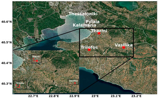
Figure 1.
Map of the greater study area and the measurement locations. The colored dots represent the location of stations installed at each site: the city center of Thermi (abbreviated as Thermi, with 6 stations), Trilofos (4 stations), and Vasilika (2 stations).
The Municipality of Thermi’s air-quality conditions are affected by local sources, mainly traffic and residential heating emissions, while the transboundary transport of pollutants due to air masses originating from central and eastern Europe may also provoke elevated PM2.5 levels [38]. Moreover, the municipality of Thermi is situated next to the metropolitan area of Thessaloniki (Figure 1), the second largest city in Greece. Thus, emissions from Thessaloniki’s urban, industrial, and port activities [39] may also have a negative contribution to the municipality of Thermi’s air-quality conditions. In general, domestic biomass burning has been identified as one of the major air-quality issues among southeastern European countries [40] and Thessaloniki [41,42,43]. This is the case also for the greater Thermi area where prolonged biomass burning activities from the residential heating sector comprise during the winter the most abundant PM source.
An Internet of Things (IoTs) monitoring system equipped with 28 low-cost PM sensors was deployed in 2018 in the greater Municipality of Thermi area, continuously monitoring and transferring information about PM concentrations (https://www.thermiair.gr/; accessed on 1 May 2024). To facilitate the analysis, the measurement sites were classified into 3 sub-regions considering their type and geographical location [44]. The three sub-regions examined in the Municipality of Thermi were: (1) the city center of Thermi (abbreviated as Thermi; 6 stations), Trilofos (4 stations), and Vasilika (2 stations).
- Thermi is in the municipality’s city center. In that area, vehicular circulation density is high and characterized as an urban-traffic region.
- Trilofos is a suburban area situated approximately 11 km south of Thermi’s city center.
- Vasilika, located 13 km southeast of Thermi, is a suburban area mainly affected by residential heating emissions.
The geographical arrangement, the characteristics, and the PM2.5 levels of the measuring areas are presented in Figure 1 and Table 1. Moreover, the hourly and daily PM2.5 levels of each measuring station are presented in Figures S1 and S2, respectively, whereas the average PM2.5 concentrations per season in the examined sites in Figure 1 are presented in Table S1. Overall, the measuring locations showed an hourly data completeness higher than 92%.

Table 1.
Information about the examined areas in Thermi during the study period (2021–2023).
Even though the proposed methodology was applied to the three distinct sites in the greater Municipality of Thermi area, for brevity, only the results for Thermi are presented in the main text, whereas the results for the two additional sites, Trilofos and Vasilika, are presented in the Supplementary Materials. Across the area, historical records showed elevated PM2.5 mass concentrations, especially during winter, and emphasize the need for better air-quality management. The forthcoming analysis focused on the period from January 2021 to December 2023. Measurements before January 2021 were not considered to avoid effects of the restriction measures due to the COVID-19 outbreak in Greece.
2.2. Data
2.2.1. PM2.5 from LCSs and CAMS
For the purpose of this study, PurpleAir (PAir) LCSs were utilized, providing continuous PM2.5 measurements. Their operation is based on the principles of light scattering and conversion of the signal to mass concentration values. An integrated fan drew ambient air through the measurement chamber where a photodiode detected scattered light that was later converted to PM concentration though a proprietary algorithm.
The PM network provides measurements in about 2 min intervals averaged over 10 min and hourly periods for the forthcoming analysis. For data validity during the hourly mean calculations, we required more than 4 (out of the total of 6) 10 min measurements. The rest of the data was flagged as invalid and was excluded from the subsequent analysis.
Hourly PM2.5 measurements were used for the development and verification of the proposed forecasting model. Several studies have investigated and evaluated these sensors, and the results point out a satisfactory performance across various environments [45,46,47]. More specifically, for the forthcoming analysis, the raw (CF = 1) PAir measurements were corrected based on the equation derived by Kosmopoulos et al. [17] to assure the network’s accuracy:
The European Copernicus Atmosphere Monitoring Service (CAMS) provides hourly air-quality forecasts for Europe on a ~10 km spatial grid with a forecast horizon up to 96 h [48]. The CAMS air-quality dataset was generated by an ensemble of eleven distinct air-quality forecasting systems spanning across Europe. A median ensemble was derived from the individual outputs providing PM2.5 measurement forecasts, aiming to achieve a better performance than the individual model products. The PM2.5 forecasts were available daily every 00 UTC. The spatial collocation between the gridded forecasts and measurements was conducted by selecting the nearest neighbor pixel of the site location (Table 1).
2.2.2. Meteorology
Meteorological parameters were acquired from the Copernicus Atmosphere Data Store using the CAMS global atmospheric composition forecasts dataset [49]. The global atmospheric composition forecasts data run twice daily from 00 and 12 UTC at hourly temporal resolutions (for surface fields) and 0.4° spatial grids. In this study, the meteorological variables used were air temperature at 2 m (T in °C), wind speed (WS in m/s), wind direction (WD in degrees), total precipitation (TP in mm), and boundary layer height (BLH in m). To extract the gridded forecasted data for the three regions, firstly, the daily forecasts for 00 UTC were selected; secondly, the average lat–lon pair of the stations included in each region (Figure 1) was calculated (Table 1); and thirdly, a nearest neighbor interpolation was applied for each lat–lon pair.
3. PM2.5 Concentration Forecasting Based on the LSTM
3.1. LSTM
The LSTM [50] constitutes a type of recurrent neural network (RNN) [51]. RNNs are superior at processing time-series data for forecasting. This lies in their ability to remember information from past occurrences that can be used to predict future patterns, making them adequate for forecasting tasks. However, RNNs frequently suffer from vanishing gradient problems, leading to slow model learning (in terms of updating neural network weights) and, in the worst scenario, stopping the learning procedure [52]. LSTM models have been developed to overcome such problems and, internally, can learn long-term dependencies, thus being a promising solution for long-term time-series forecasting [53]. A reference LSTM architecture is depicted in Figure 2a.
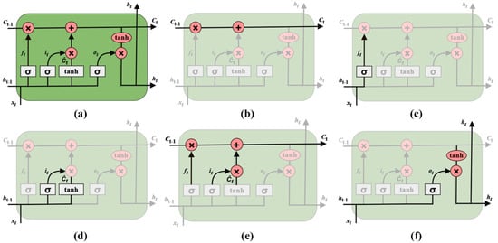
Figure 2.
(a) Long short-term memory (LSTM) neural network architecture. (b) The cell state, (c) the forget gate, (d) the first step of the input gate, (e) the second step of the input gate, and (f) the output gate of an LSTM architecture. The white rectangles correspond to a neural network layer, while the red elliptic shapes correspond to a pointwise operation.
The diagram in Figure 2a particularly describes a memory block, where the core idea is to transfer information through the cell state (Figure 2b; the horizontal line running through the top of the diagram), which is weighted based on its significance. The information added or removed from the cell state is regulated by the so-called gates. An LSTM includes three of these gates, namely the input, forget, and output gates. In the following paragraphs, the LSTM implementation will be thoroughly presented in steps.
The first step of the LSTM application involves the amount of information that is to be removed by the cell state (forget gate; Figure 2c). The latter is accomplished using Equation (2):
where σ is the sigmoid function (Equation (3)):
The next step is to choose which new information will advance through the new cell state (input gate; Figure 2d,e). This is performed in two steps: first, a sigmoid layer determines which values will be updated (Equation (4)), and second, a tanh layer creates a vector of new potential values (Equation (5)):
The following step is to update the cell state, Ct−1, with a new weighted cell state, Ct, based on Equation (6):
The first part of Equation (6) corresponds to the amount of information that will be forgotten by the old cell state, Ct−1, whilst the second part of Equation (6) refers to the amount of information that will be updated.
The last step is to decide the output values (output gate; Figure 2f). This is conducted in two steps: first, a sigmoid layer is applied, which decides what parts of the cell state will be the output (Equation (7)), and second, the tanh function is applied to the cell state, scaling the values between −1 and 1, and then multiplying it by the output of the sigmoid gate (Equation (8)), so that the only output is the parts that are decided.
3.2. Methodology
The proposed methodology for PM2.5 forecasting is illustrated in Figure 3. To achieve the “best” LSTM network architecture, various tests were applied, seeking an optimal configuration of hyperparameters, such as the number of (1) hidden layers, (2) nodes in each hidden layer, (3) epoch, (4) batch size, and (5) length of the time input sequence. In addition, the most suitable optimizer, loss, and activation functions were investigated. The optimal configuration for these hyperparameters for each region was determined through a group of various range values, resulting in the “best” LSTM network architecture (see Section 3.3).
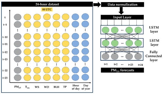
Figure 3.
Methodology of PM2.5 LSTM forecasting. The 24 h sliding-window dataset consists of the closest meteorological forecasted data at 00 UTC.
3.2.1. Input Parameters
The applied methodology consisted of three main categories of input parameters, (1) PM2.5, (2) meteorological variables, and (3) time variables, all related to air pollution. The major auxiliary predictor parameters (except LCSs PM2.5) in the applied methodology were the meteorological forecasts from CAMS.
In polluted areas, temperature has a negative relationship to PM2.5 concentrations for low temperatures and a positive relationship for high temperatures [54]. Temperature affects fuel usage and chemical reactions in the atmosphere [36]. Wind speed presents a negative correlation with PM2.5 due to its ability to carry air pollutants away from their source, causing ambient particle dispersion, provoking lower PM2.5 concentrations for higher wind-speed values [55]. Wind direction is an important meteorological variable for detecting the location of the air pollution source. Boundary-layer height controls the volume available for pollution dispersion and movement in the lower atmosphere [56]. Low values and weak turbulence enhance the accumulation of air pollutants. Precipitation reveals a negative correlation with PM2.5 concentrations due to wet deposition mechanisms.
Two additional variables were included to describe the intra-day and yearly emissions variability. The day of the year was applied to reproduce the seasonal variations in emissions, and the hour of the day was used to capture the variability of city activities within the day that affected air pollution.
3.2.2. Data Preprocessing
Data were adequately preprocessed for the optimal training of the model. In particular, the input variables, as described in Section 3.2.1, were applied as 24 h data sequences. The time lag of 24 was selected because a continuous and repeated pattern was revealed for the PM2.5 autocorrelation for every 24 h (Figure S3). The latter means that the PM2.5 observations were highly correlated for this period, and the value of 24 was suitable as a time-lag value. As was mentioned in Section 2.2.2, the forecasted meteorological data were available daily at 00 and 12 UTC at a 1 h temporal resolution. In this study, the 24 h meteorological data sequences were constructed using the closet forecasted data at 00 UTC. For model training, the 24 h data sequences were generated in sliding windows of 1 h, aiming to forecast PM2.5 concentrations 24 h in advance. WD was classified into sixteen sectors and was used as categorical data. Prior to model training, the non-categorical feature parameters underwent normalization between 0 and 1 using the Min–Max normalization method.
3.2.3. Methodology Configuration
The dataset was split into two parts before the development of the LSTM model: the training and testing datasets. The 2021–2022 period was allocated for the training dataset, while 2023 for testing. The training set during the training of the model was again divided into two datasets: 90% of the training dataset was used for training the model and the other 10% for model validation. The model used has two LSTM layers (Figure 2), each with 64 nodes activated through the tanh function, and a fully connected linear output layer (Figure 3). The Adam optimizer was applied, encompassing the minimum error with the least number of epochs (50). Regarding validation loss, the mean absolute error was preferred for the tuning of the LSTM.
The same model’s hyperparameter tuning revealed the same configuration for each of the three regions. The outputs (1–24 h ahead, as mentioned in Section 3.2.2) of each model forecast were daily averaged for examining the presence of daily PM2.5 exceedances. The detailed methodology configuration, including all the LSTM’s parameters, is presented in Table S2.
3.3. Model Evaluation
The assessment of PM2.5 forecasts was performed using the mean absolute error (MAE), root mean square error (RMSE), and Pearson correlation coefficient (R) that are defined by:
Additionally, the qualitative performance of the forecasted PM2.5 exceedances was assessed using the following metrics:
The above metrics (Equations (12)–(14)) can easily be understood by using the following confusion matrix (Figure 4).
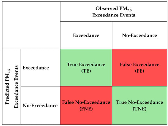
Figure 4.
Confusion matrix of possible cases of forecasted PM2.5 exceedance events.
The diagonal elements of the confusion matrix (Figure 4) represent the correctly detected exceedance/no-exceedance events (true exceedance, TE, and true no-exceedance, TNE). The off-diagonal values indicate erroneous predictions for the presence or absence of TE (false exceedance, FE, and false no-exceedance, FNE) using the daily average PM2.5 forecast.
4. Results
4.1. PM2.5 Concentrations and Meteorology
The average monthly PM2.5 concentrations in Thermi in 2021–2023 are presented separately for each year in Figure 4. During the warm season (April to October), PM2.5 levels in Thermi remain stable, with monthly average concentrations remaining lower than 10 μg m−3 (Figure 4). Impaired air-quality conditions were reported during the colder period (November to March). Especially during January and December, PM2.5 levels remain higher than 12 μg m−3, reaching up to approximately 22 μg m−3 (January 2022). Transportation and residential heating emissions (biomass burning) are the primary local PM2.5 sources during these months. A common seasonal pattern was also identified across other regions (Trilofos and Vasilika). For clarity, the results of the analysis from these two regions are shown in the Supplementary Materials (Figures S4a and S5a).
The diurnal variability of PM2.5 concentrations in Thermi is depicted in Figure 5. The PM2.5 cycle exhibited a modest peak around 05:00–07:00 (UTC), due to the morning rush hour, and then a nighttime peak at 17:00–21:00 (UTC) that is highly associated with local biomass burning emissions, due to the increased heating needs during the colder period (November to March). Higher hourly values were revealed for the training years (2021 and 2022) than the testing period (2023). The discrepancy between the periods is more apparent for the nighttime peak. The corresponding diurnal variabilities for Trilofos and Vasilika are shown in Figures S4b and S5b.
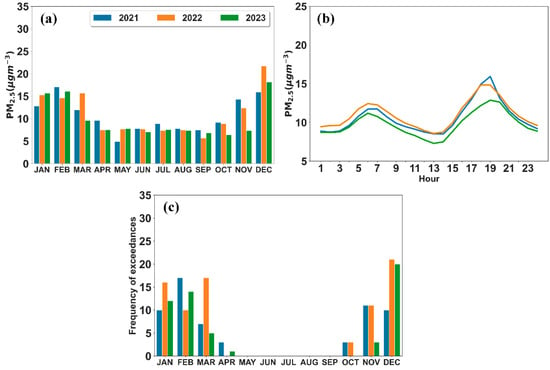
Figure 5.
(a) Monthly and (b) diurnal variabilities of PM2.5 concentrations, and (c) frequency of daily WHO exceedances in Thermi per year in the 2021–2023 study period.
In 2021–2023, several exceedances of the WHO-regulated daily limits (15 μg m−3) were reported in all areas during both seasons (Figure 5c, Figures S4c and S5c). The number of exceedance days in Thermi was higher during the wintertime (December to February), as it was expected due to the lower temperatures and the increased heating needs. During that period, the observed exceedance episodes were more than 10, for each month, and reached up to 21 in January 2022. These elevated PM2.5 pollution episodes underline the importance of local emissions and the need for better air-quality management mechanisms that should be put into place.
Figure 6 shows the mean monthly temperature values as well as the diurnal variability of the boundary-layer height and the wind speed and direction during the study period in the study area, separated into warm and cold periods. A strong monthly temperature variability was documented, including records that varied from 2 °C to 27 °C from January (winter) to July (summer). Throughout the colder period, the predominant wind direction was northwest, favoring long-range PM2.5 transportation from other European cities and, specifically, Thessaloniki (located in the northwest of the Municipality of Thermi) to the study region. During the warm period, northwest (less intense than the colder period) and south-southeast winds were identified as the prevailing winds. Consequently, the examined area could also be affected by long-range transport from southern European source regions. In addition, notable differences in the boundary-layer height are presented between the two periods (Figure 6). The diurnal cycle of boundary-layer height was stronger during the warm period, increasing the dispersion and movement of atmospheric pollution into the lower atmosphere. On the contrary, a confined range of BLH was documented in the cold period, revealing values between 200 m during the sunless hours and 800 m at noon.
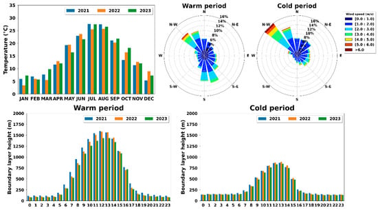
Figure 6.
Monthly variations in temperature (top left), wind in warm period (top middle) and cold period (top right), and boundary-layer height in warm period (bottom left) and cold period (bottom right).
4.2. Forecasting PM2.5 Performance
The hour-by-hour forecasting performance of the applied methodology is presented in Figure 7. The analysis was conducted for 2023 (Figure 7) as well as separately for the warm (Figure 7b) and cold (Figure 7c) periods. The following performance indicators, RMSE, MAE, and R, were calculated and used as the error evaluation indices of the LSTM’s performance for various forecasting periods (from 1 h ahead up to 24 h).
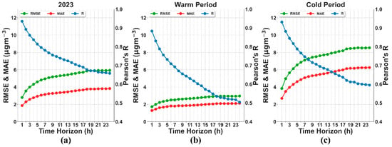
Figure 7.
LSTM evaluation metrics, MAE, RMSE (μg m−3), and R, in Thermi, during (a) 2023, (b) the warm period (April–October), and (c) cold period (November–March).
Based on Figure 7, the forecast horizon clearly affected the model’s performance, especially at short time horizons (up to 5 h). Taking into account the whole testing period (2023), the correlation between the measured PM2.5 values and the LSTM forecast data ranges between 0.67 and 0.94 for all time horizons, revealing a decreasing trend as the time horizon increases (Figure 7a). As expected, the LSTM revealed a better forecasting performance at short time horizons (R > 0.8 up to 5 h). The cold period yielded similar results, while the warm period revealed lower R values at higher forecast horizons. For the Trilofos and Vasilika regions, similar results were reported, with the only differences being the slightly lower R values at short time horizons presented in Vasilika (Figures S6 and S7).
After the first hour, the MAE and RMSE evaluation metrics increased gradually with time, indicating the highest bias of the estimations compared to the actual observations generated by the proposed LSTM model. A sharp reduction in the model’s performance (MAE and RMSE) was observed during the subsequent hours, from 1 to 9 h (from 1.9 to 3.5 and from 3.2 to 5.9 μg m−3). After these breakpoints, the MAE and RMSE curves were more flat, denoting a less-pronounced performance deterioration. In general, the RMSE and MAE recorded ~2 μg m−3-higher values in Vasilika than in Thermi and Trilofos due to the higher observed PM2.5 levels (Figure S5). Despite the increment in evaluation indices and the slightly lower accuracy, we can observe that the model’s efficiency remains quite reasonable in all the examined areas.
The accuracy of the proposed methodology was also evaluated against the PM2.5 forecasts from CAMS (Figure S8). To compare the two different forecasting products, the metrics were calculated by using the hourly LSTM PM2.5 concentrations with a starting forecast time of 00 UTC to match the temporal resolution of CAMS, which was provided at that time. The two products revealed the same metrics pattern as the time horizon increased, reflecting the diurnal variability of air quality across the study regions. The LSTM forecasts included lower RMSE, MAE, and higher R metrics than CAMS, especially across the morning and nighttime rush hours, where the PM2.5 concentrations were highly variable. For instance, LSTM R values in Thermi ranged from 0.55 to 0.92 (average = 0.72), while CAMS revealed a poorly R range between 0.52 and 0.65 (average = 0.57).
The performance of the applied methodology in reproducing the diurnal cycle of PM2.5 mass concentration was investigated by calculating the mean hourly PM2.5 forecasts and measurements, including their deviations, as depicted in Figure 8. The diurnal fluctuations in PM2.5 concentrations were calculated using the forecasts with a starting forecast time of 00 UTC. The proposed model PM2.5 forecasts demonstrate a remarkable performance in capturing the diurnal cycle of air pollution, particularly during nighttime hours when Thermi experiences the highest concentration levels. The LSTM seems to slightly overestimate the measurements by ~2 μg m−3 during the cold period at morning rush hour.
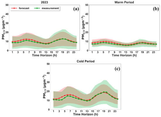
Figure 8.
Comparison of the diurnal variability between LSTM PM2.5 forecasts and PM2.5 measurements in Thermi during (a) 2023, (b) the warm period (April–October), and (c) cold period (November–March).
4.3. Forecasting Air Pollution Exceedances
The WHO-regulated daily PM2.5 threshold was assessed to evaluate the forecasting system’s efficiency more thoroughly in pollution-level estimations. Several WHO daily limit exceedances were reported in the examined areas during the study period (2021–2023), as shown in Figure 5c, Figures S4 and S5c. To investigate the LSTM exceedance forecast performance, daily PM2.5 concentrations were calculated using the forecasts with a starting forecast time of 00 UTC. If the daily averaged forecasted PM2.5 value exceeds the WHO predefined threshold limit (15 μg m−3), then an air pollution exceedance event occurs. The purpose and utility of the proposed PM2.5 forecasting lie in the implementation of better and improved air-quality management techniques. Thus, it is crucial to evaluate the LSTM’s daily exceedance prediction skills.
The overall performance of the applied methodology to capture the daily air pollution exceedances in Thermi is depicted in Figure 9. The results for the two additional sites are presented in Figures S9 and S10. The proposed LSTM forecasting system reported a high percentage of correctly forecasted exceedances and no exceedances during the whole year. The proposed methodology’s total accuracy during the test period (2023) was approximately 92%. More specifically, the LSTM forecasting system correctly captured 83.3% of the air pollution exceedance events in Thermi. This portion corresponds to the accurate identification of 45 daily limit exceedance incidents. The analysis also denotes the feasibility and response of the proposed algorithm to capture day to day PM2.5 level variations.
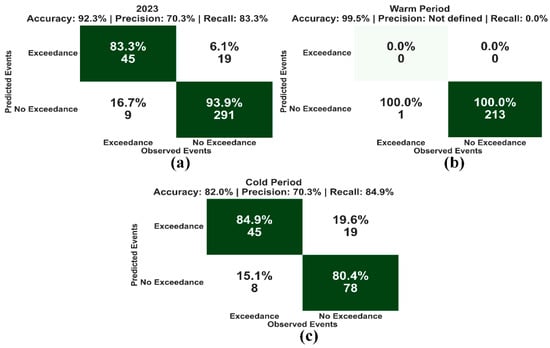
Figure 9.
Confusion matrix for all possible cases in Figure 4. Table S3 in Thermi during (a) 2023, (b) the warm period (April–October), and (c) cold period (November–March). The percentages of each quadrant are calculated based on the true measured cases (either for exceedance or no-exceedance events) and refer only to the forecasts starting at 00 UTC, including 24 h days in 2023 (testing period).
As has already been discussed in previous sections, degraded air-quality conditions in Thermi were reported during the colder months (November to March). Thus, it would be useful to characterize the systems’ forecasted exceedance and no-exceedance accuracies separately for each season. During the warmer months (April to October) in 2023, there was only one daily exceedance reported by the monitoring network (Figure 9b). That event, though, was not captured by the LSTM algorithm. The low PM2.5 concentrations reported during the previous hours may have led to that inability. Eventually, the system’s accuracy in forecasting no-exceedance events was expected since the hourly and daily fluctuations were minimized during that period.
On the contrary, the model’s performance was ameliorated during the colder period (November to March), when a significant increase in exceedances was exhibited. As denoted in Figure 9c, the proposed algorithm accurately reports 45 out of the total 64 daily exceedances of the WHO-regulated thresholds (~85% of the exceedances). Moreover, during these months, almost 81% of the no-exceedance events (78 out of the 85) were also correctly identified, leading to a total accuracy of 82%. Since degraded air-quality conditions in the examined Thermi region occur almost exclusively during the winter months, it is important to highlight the better performance of the proposed LSTM forecasting algorithm during that period.
The latter findings underlie the model’s capabilities to correctly detect possible WHO threshold exceedances and provide valid information concerning the local air quality in real-time conditions.
The false-alarm probabilities, during the whole year, remained low (6.1%) in Thermi. In cases where the model fails to correctly predict exceedances or non-exceedances, the model tends to overestimate the PM2.5 concentrations by 4.2 μg m−3. The quality of the reported results highlights the utility of the proposed forecasting system within the context of the dissemination of early warnings to the public and stakeholders and tackling or even eliminating PM air pollution-related problems.
The monthly variability of the correctly captured exceedances using the LSTM (Figure 10a) and CAMS (Figure 10b) forecasts was further investigated in Thermi as well as for the other two sites in Figures S11 (Trilofos) and S12 (Vasilika). During the winter months (December to February), the LSTM forecasting performance was adequately good, ranging between 84.2% and 100.0%, capturing, in total, 40 out of 45 exceedances. At the same time, the CAMS can correctly capture 32 out of 45 exceedances, documenting a range between 63.1% and 85.7%, lower than the proposed methodology. Both forecasting methodologies failed to capture the one exceedance case in April. In Trilofos, the results were similar to those in Thermi (Figure S11). Nevertheless, at the Vasilika site, the CAMS failed to capture the majority of the exceedance cases, while the LSTM revealed a superior performance, capturing 59 out of 63 cases (>84.0%) during the winter months (Figure S12).

Figure 10.
Monthly variability of the true predicted exceedances from (a) the LSTM and (b) CAMS PM2.5 forecasts in Thermi.
Figure 11 presents the daily PM2.5 concentrations as derived by the forecasting system (black bars) and the monitoring network (purple bars). The diagram also visualizes the European AQI as provided by the European Environment Agency (EEA) and the European Commission. The use of this index facilitates the evaluation of the LSTM’s overall forecasting performance for different PM2.5 levels. For clarity, we present the results during the 4 months of the testing period (2023) representative of each season, namely January for winter, April for spring, July for summer, and October for autumn. These months accurately represent the seasonal magnitude of and daily variations in PM2.5 concentrations during the year.
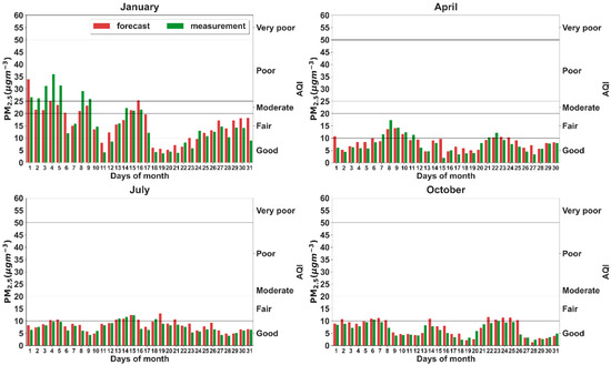
Figure 11.
Daily average forecasted (LSTM, red bars) and observed (LCSs, green bars) PM2.5 concentrations during January, April, July, and October 2023 in Thermi. The second axis along with the horizontal, black, solid lines categorize the AQI.
The daily time series indicate that, regardless of the month or the season, the forecasting system’s performance is adequately good. It is apparent that the estimated PM2.5 concentrations are in good agreement with the measured ones. The LSTM captures the daily PM2.5 cycle of the actual values without a clear underestimation or overestimation trend. Moreover, the model captured the daily variability of the observed data.
In January, when elevated PM2.5 levels were recorded due to biomass burning emissions in Thermi and a shallower nocturnal boundary layer, the model produced accurate forecasts with small discrepancies against the measured values. During the days with PM2.5 concentrations higher than 15 μg m−3, the LSTM tended to slightly overestimate the peak values in Thermi (MBE = 1.02 μg m−3), but for the majority of the days (~70% of the days), the forecasting system predicted the AQI correctly. This finding underlines the forecasting capabilities of such RNNs compared to the statistical models that traditionally tend to systematically underpredict extreme pollution events [57].
During the non-winter months, PM2.5 remained lower than 20 μg m−3 in all cases, suggesting common daily fluctuations. The system can operate robustly during summer (July), when all days correspond to low PM2.5 concentrations (<12 μg m−3) and the weather conditions are rather stable. A comparison between the predicted values and the measured ones indicates a good predictive capability and, in general, a better forecasting skill during periods without abrupt PM2.5 changes. Finally, in October, the developed model’s performance was similar and capable of properly forecasting air-quality values.
Regarding the system’s capability to identify the WHO daily limit exceedances, Figure 12 presents the predicted exceedances for each day of the month in 2023.

Figure 12.
Calendar plot for all possible cases in Figure 4 in Thermi. Missing data are presented in black.
As has already been discussed, the examined area experienced higher PM2.5 concentrations during the colder months; thus, the occurrence of the exceedances was reported during that time of the year. Figure 12 shows the seasonal variability of the PM2.5 exceedance frequency reported by the LSTM system against the measurements. The system performance exhibits high similarity and a common temporal pattern. The increased number of exceedances accumulated during December, January, and February, when more than 50 daily exceedances were reported in all areas. During that period, the forecast algorithm reported a success rate higher than 75% of daily exceedances.
5. Discussion
Since PM air pollution poses one of the most important environmental issues affecting global health and ecosystems, effective policies are necessary to lower the burden of PM-related adverse effects. The development of numerous, commercial, low-cost PM sensors during the last decade has facilitated the continuous real-time monitoring of particles’ ambient concentrations and the identification of their spatiotemporal variations and source identification. Despite the comprehensive insights provided by such dense networks, there is still a lack of awareness among citizens regarding the association between the poor air quality we breathe and the potential health effects.
An effective method to bridge this gap and implement more effective policies could be the adoption of early warning PM forecasting systems as an aid in decision making. Knowing, in advance, the probability of exceedances of the regulated PM limits could be a valuable tool for sensitive groups of people (e.g., kids, the elderly, and those with asthma), allowing them to plan their activities and reduce their exposure. Minimizing people’s exposure to elevated PM levels could reduce health risks and could help them increase their environmental consciousness.
The proposed PM2.5 forecasting algorithm could be integrated into already existing monitoring networks as a valuable air-quality early warning system. It could be a valuable and effective tool to stakeholders and air-quality management experts to implement countermeasures to safeguard public health. The application of such a forecasting algorithm would allow citizens, and especially vulnerable groups, i.e., children, elderly, and people with asthma or allergies, to reduce or tailor their outdoor activities based on intra-hour or daily PM2.5 level forecasts. The synergy of continuous monitoring and early warning could be the basis for better mitigation strategies toward achieving more effective environmental and public health protection techniques.
6. Conclusions
Reliable air pollution forecasting has gained more attention recently to offer accurate information on air-quality levels because of the critical implications high PM2.5 concentrations have on the environment and human health. To improve the decision-making process for required mitigation and to warn the public early on, accurate and practical air-quality forecasting is also essential. In this study, an LSTM-based model was proposed to forecast 1 h PM2.5 concentrations across urban and suburban environments (Municipality of Thermi, Greece). The proposed LSTM approach uses, except for PM2.5 measurements, two groups of auxiliary data, such as meteorological data, like the temperature, wind speed and direction, precipitation, and boundary-layer height, and time variables, like the hour of the day and the day of the year, to enhance forecasting accuracy.
The forecasting performance of PM2.5 concentrations in terms of correlation was between 0.67 and 0.94 at all-time horizons, revealing a decreasing trend as the time horizon increased. PM2.5 concentration forecasts were further used to detect possible WHO threshold exceedances and provide valid information concerning the local air quality. The LSTM forecasting system can correctly capture more than 71.0% of the air pollution exceedance events in the urban area. Despite the good accuracy of the LSTM model to capture air pollution exceedance events, it can also avoid false-alarm probabilities, with cases lower than 8% in the broader area. The findings of this work anticipate that hourly PM2.5 concentration forecasting as well as the accurate detection of possible WHO threshold exceedances will be of great significance for the citizens in the larger area as they can provide vital information about heavy air pollution days.
Supplementary Materials
The following supporting information can be downloaded at: https://www.mdpi.com/article/10.3390/atmos15050594/s1, Figure S1: Hourly time series of PM2.5 concentrations at the stations in Thermi, Trilofos, and Vasilika; Figure S2: Daily time series of PM2.5 concentrations at the stations in Thermi, Trilofos, and Vasilika; Figure S3: Autocorrelation coefficient of PM2.5 observations of different delay times; Figure S4: Same as Figure 5 for Trilofos; Figure S5: Same as Figure 5 for Vasilika; Figure S6: Same as Figure 7 for Trilofos; Figure S7: Same as Figure 7 for Vasilika; Figure S8: LSTM and CAMS evaluation metrics, MAE, RMSE (μg m−3), and R for Thermi in 2023, taking into account the 24 h forecasts at 00 UTC; Figure S9: Same as Figure 9 for Trilofos; Figure S10: Same as Figure 9 for Vasilika; Figure S11: Same as Figure 10 for Trilofos; Figure S12: Same as Figure 10 for Vasilika; Figure S13: Same as Figure 11 for Trilofos; Figure S14: Same as Figure 11 for Vasilika; Table S1. Average PM2.5 concentrations (±standard deviation) during winter, spring, summer, and autumn in the 14 examined sites in Thermi. The averaged values have been calculated from the daily data; Table S2: LSTM configuration.
Author Contributions
Conceptualization, S.-A.L., G.K., O.P. and V.S.; methodology S.-A.L. and G.K.; software, S.-A.L.; validation, S.-A.L., G.K. and V.S.; formal analysis, S.-A.L.; investigation, V.S and A.K.; resources, G.K. and A.K.; data curation, S.-A.L. and G.K.; writing—original draft preparation, S.-A.L. and G.K.; writing—review and editing, S.-A.L., G.K., O.P., V.S. and A.K.; visualization, S.-A.L.; supervision, A.K. and V.S.; project administration, A.K.; funding acquisition, A.K. All authors have read and agreed to the published version of the manuscript.
Funding
This research received no external funding.
Institutional Review Board Statement
Not applicable.
Informed Consent Statement
Not applicable.
Data Availability Statement
Simulation dataset can be provided upon request. The CAMS meteorological and air pollution forecast data used in this study were derived from the following resources available in the public domain: https://ads.atmosphere.copernicus.eu/ (accessed on 12 May 2024).
Acknowledgments
We acknowledge the support of this work by the “Thermi-Air: Investigation of spatial and temporal variability in concentrations of airborne particulate matter in the Municipality of Thermi with emphasis on the potential impact on citizens’ health” project, supported by the Municipality of Thermi.
Conflicts of Interest
The authors declare no conflicts of interest.
References
- Manisalidis, I.; Stavropoulou, E.; Stavropoulos, A.; Bezirtzoglou, E. Environmental and Health Impacts of Air Pollution: A Review. Front. Public Health 2020, 20, 14. [Google Scholar] [CrossRef] [PubMed]
- Johnston, F.H.; Borchers-Arriagada, N.; Morgan, G.G.; Jajaludin, B.; Palmer, A.J.; Williamson, G.K.; Bowman, D.M.J.S. Unprecedented health costs of smoke-related PM2.5 from the 2019–2020 Australian megafires. Nat Sustain. 2021, 4, 42–47. [Google Scholar] [CrossRef]
- Lee, Y.G.; Lee, P.H.; Choi, S.M.; An, M.H.; Jang, A.S. Effects of Air Pollutants on Airway Diseases. Int. J. Environ. Res. Public Health 2021, 18, 9905. [Google Scholar] [CrossRef] [PubMed]
- World Health Organization (WHO). Fact Sheet: Ambient (Outdoor) Air Pollution. 2022. Available online: https://www.who.int/news-room/fact-sheets/detail/ambient-(outdoor)-air-quality-and-health/ (accessed on 15 January 2024).
- Masson-Delmotte, V.; Zhai, P.; Connors, S.L.; Péan, C.; Berger, S. IPCC, 2021: Climate change 2021: The physical science basis. In Contribution of Working Group I to the Sixth Assessment Report of the Intergovernmental Panel on Climate Change; Cambridge University Press: Cambridge, UK; New York, NY, USA, 2021; pp. 3–32. [Google Scholar] [CrossRef]
- Nada Osseiran, Christian Lindmeier: 9 out of 10 People Worldwide Breathe Polluted Air, but More Countries Are Taking Action. 2018. Available online: https://www.who.int/news/item/02-05-2018-9-out-of-10-people-worldwide-breathe-polluted-air-but-more-countries-are-taking-action (accessed on 12 May 2023).
- World Health Organization. WHO Global Air Quality Guidelines: Particulate Matter (PM2.5 and PM10), Ozone, Nitrogen Dioxide, Sulfur Dioxide and Carbon Monoxide World Health Organization. 2021. Available online: https://apps.who.int/iris/handle/10665/345329 (accessed on 12 May 2023).
- European Environment Agency. Exceedance of Air Quality Standards in Europe. 2022. Available online: https://www.eea.europa.eu/ims/exceedance-of-air-quality-standards (accessed on 20 December 2022).
- Kumar, P.; Morawska, L.; Martani, C.; Biskos, G.; Neophytou, M.; Di Sabatino, S.; Bell, M.; Norford, L.; Britter, R. The Rise of Low-Cost Sensing for Managing Air Pollution in Cities. Environ. Int. 2015, 75, 199–205. [Google Scholar] [CrossRef] [PubMed]
- Morawska, L.; Thai, P.K.; Liu, X.; Asumadu-Sakyi, A.; Ayoko, G.; Bartonova, A.; Bedini, A.; Chai, F.; Christensen, B.; Dunbabin, M.; et al. Applications of Low-Cost Sensing Technologies for Air Quality Monitoring and Exposure Assessment: How Far Have They Gone? Environ. Int. 2018, 116, 286–299. [Google Scholar] [CrossRef]
- Giordano, M.R.; Malings, C.; Pandis, S.N.; Presto, A.A.; McNeill, V.F.; Westervelt, D.M.; Beekmann, M.; Subramanian, R. From low-cost sensors to high-quality data: A summary of challenges and best practices for effectively calibrating low-cost particulate matter sensors. J. Aerosol Sci. 2021, 158, 105833. [Google Scholar] [CrossRef]
- Zimmerman, N. Tutorial: Guidelines for implementing low-cost sensor networks for aerosol monitoring. J. Aerosol Sci. 2022, 159, 105872, ISSN 0021-8502. [Google Scholar] [CrossRef]
- Zheng, T.; Bergin, M.H.; Johnson, K.K.; Tripathi, S.N.; Shirodkar, S.; Landis, M.S.; Sutaria, R.; Carlson, D.E. Field evaluation of low-cost particulate matter sensors in high- and low-concentration environments. Atmos. Meas. Tech. 2018, 11, 4823–4846. [Google Scholar] [CrossRef]
- Bulot, F.M.J.; Johnston, S.J.; Basford, P.J.; Easton, N.H.C.; Apetroaie-Cristea, M.; Foster, G.L.; Morris, A.K.R.; Cox, S.J.; Loxham, M. Long-term field comparison of multiple low-cost particulate matter sensors in an outdoor urban environment. Sci. Rep. 2019, 9, 7497. [Google Scholar] [CrossRef]
- Kang, Y.; Aye, L.; Ngo, T.D.; Zhou, J. Performance Evaluation of Low-Cost Air Quality Sensors: A Review. Sci. Total Environ. 2022, 818, 151769. [Google Scholar] [CrossRef]
- DeSouza, P.; Kahn, R.; Stockman, T.; Obermann, W.; Crawford, B.; Wang, A.; Crooks, J.; Li, J.; Kinney, P. Calibrating networks of low-cost air quality sensors. Atmos. Meas. Tech. 2022, 15, 6309–6328. [Google Scholar] [CrossRef]
- Kosmopoulos, G.; Salamalikis, V.; Pandis, S.N.; Yannopoulos, P.; Bloutsos, A.A.; Kazantzidis, A. Low-cost sensors for measuring airborne particulate matter: Field evaluation and calibration at a South-Eastern European site. Sci. Total Environ. 2020, 748, 141396. [Google Scholar] [CrossRef] [PubMed]
- Considine, E.M.; Reid, C.E.; Ogletree, M.R.; Dye, T. Improving accuracy of air pollution exposure measurements: Statistical correction of a municipal low-cost airborne particulate matter sensor network. Environ. Pollut. 2021, 268, 115833. [Google Scholar] [CrossRef] [PubMed]
- Rose Eilenberg, S.; Subramanian, R.; Malings, C.; Hauryliuk, A.; Presto, A.A.; Robinson, A.L. Using a network of lower-cost monitors to identify the influence of modifiable factors driving spatial patterns in fine particulate matter concentrations in an urban environment. J. Expo. Sci. Environ. Epidemiol. 2020, 30, 949–961. [Google Scholar] [CrossRef] [PubMed]
- Lu, Y.; Giuliano, G.; Habre, R. Estimating hourly PM2.5 concentrations at the neighborhood scale using a low-cost air sensor network: A Los Angeles case study. Environ. Res. 2021, 195, 110653. [Google Scholar] [CrossRef] [PubMed]
- Frederickson, L.B.; Sidaraviciute, R.; Schmidt, J.A.; Hertel, O.; Johnson, M.S. Are dense networks of low-cost nodes really useful for monitoring air pollution? A case study in Staffordshire. Atmos. Chem. Phys. 2022, 22, 13949–13965. [Google Scholar] [CrossRef]
- Keller, C.A.; Knowland, K.E.; Duncan, B.N.; Liu, J.; Anderson, D.C.; Das, S.; Lucchesi, R.A.; Lundgren, E.W.; Nicely, J.M.; Nielsen, E.; et al. Description of the NASA GEOS Composition Forecast Modeling System GEOS-CF v1.0. J. Adv. Model. Earth Syst. 2021, 13, e2020MS002413. [Google Scholar] [CrossRef]
- Copernicus Atmosphere Monitoring Service (CAMS) PM2.5 Global Forecasts. Available online: https://atmosphere.copernicus.eu/data (accessed on 22 March 2024).
- Marécal, V.; Peuch, V.; Andersson, C.; Andersson, S.; Arteta, J.; Beekmann, M.; Benedictow, A.; Bergström, R.; Bessagnet, B.; Cansado, A.; et al. A regional air quality forecasting system over Europe: The MACC-II daily ensemble production. Geosci. Model Dev. 2015, 8, 2777–2813. [Google Scholar] [CrossRef]
- Siouti, E.; Skyllakou, K.; Kioutsioukis, I.; Patoulias, D.; Apostolopoulos, I.D.; Fouskas, G.; Pandis, S.N. Prediction of the Concentration and Source Contributions of PM2.5 and Gas-Phase Pollutants in an Urban Area with the SmartAQ Forecasting System. Atmosphere 2024, 15, 8. [Google Scholar] [CrossRef]
- Bertrand, J.M.; Meleux, F.; Ung, A.; Descombes, G.; Colette, A. Technical note: Improving the European air quality forecast of the Copernicus Atmosphere Monitoring Service using machine learning techniques. Atmos. Chem. Phys. 2023, 23, 5317–5333. [Google Scholar] [CrossRef]
- Huang, Y.; Zhang, X.; Li, Y. A Novel Hybrid Model for PM2.5 Concentration Forecasting Based on Secondary Decomposition Ensemble and Weight Combination Optimization. IEEE 2023, 11, 119748–119765. [Google Scholar] [CrossRef]
- Murillo-Escobar, J.; Sepulveda-Suescun, J.P.; Correa, M.A.D. Orrego-Metaute, M.A. Forecasting concentrations of air pollutants using support vector regression improved with particle swarm optimization: Case study in Aburrá Valley, Colombia. Urban Clim. 2019, 29, 100473, ISSN 2212-0955. [Google Scholar] [CrossRef]
- Yang, J.; Yan, R.; Nong, M.; Liao, J.; Li, F.; Sun, W. PM2.5 concentrations forecasting in Beijing through deep learning with different inputs, model structures and forecast time. Atmos. Pollut. Res. 2021, 12, 101168, ISSN 1309-1042. [Google Scholar] [CrossRef]
- Sun, W.; Zhang, H.; Palazoglu, A.; Singh, A.; Zhang, W.; Liu, S. Prediction of 24-h-average PM2.5 concentrations using a hidden Markov model with different emission distributions in Northern California. Sci. Total Environ. 2013, 443, 93–103. [Google Scholar] [CrossRef]
- Perez, P.; Gramsch, E. Forecasting hourly PM2.5 in Santiago de Chile with emphasis on night episodes. Atmos. Environ. 2016, 124, 22–27. [Google Scholar] [CrossRef]
- Li, X.; Peng, L.; Yao, X.; Cui, S.; Hu, Y.; You, C.; Chi, T. Long Short-Term Memory Neural Network for Air Pollutant Concentration Predictions: Method Development and Evaluation. Environ. Pollut. 2017, 231, 997–1004. [Google Scholar] [CrossRef]
- Chiou-Jye, H.; Ping-Huan, K. A Deep CNN-LSTM Model for Particulate Matter (PM2.5) Forecasting in Smart Cities. Sensors 2018, 18, 2220. [Google Scholar] [CrossRef]
- Zhao, J.; Deng, F.; Cai, Y.; Chen, J. Long short-term memory—Fully connected (LSTM-FC) neural network for PM2.5 concentration prediction. Chemosphere 2019, 220, 486–492. [Google Scholar] [CrossRef]
- Zhang, Z.; Johansson, C.; Engardt, M.; Stafoggia, M.; Ma, X. Improving 3-day deterministic air pollution forecasts using machine learning algorithms. Atmos. Chem. Phys. 2024, 24, 807–851. [Google Scholar] [CrossRef]
- Pappa, A.; Kioutsioukis, I. Forecasting Particulate Pollution in an Urban Area: From Copernicus to Sub-Km Scale. Atmosphere 2021, 12, 881. [Google Scholar] [CrossRef]
- Giannaros, T.M.; Melas, D. Study of the urban heat island in a coastal Mediterranean City: The case study of Thessaloniki, Greece. Atmos. Res. 2012, 118, 103–120. [Google Scholar] [CrossRef]
- Kazadzis, S.; Bais, A.; Amiridis, V.; Balis, D.; Meleti, C.; Kouremeti, N.; Zerefos, C.S.; Rapsomanikis, S.; Petrakakis, M.; Kelesis, A.; et al. Nine years of UV aerosol optical depth measurements at Thessaloniki, Greece. Atmos. Chem. Phys. 2009, 7, 2091–2101. [Google Scholar] [CrossRef]
- Saraga, D.E.; Tolis, E.I.; Maggos, T.; Vasilakos, C.; Bartzis, J.G. PM2.5 source apportionment for the port city of Thessaloniki, Greece. Sci. Total Environ. 2019, 650, 2337–2354. [Google Scholar] [CrossRef] [PubMed]
- European Environment Agency. Emissions from Road Traffic and Domestic Heating behind Breaches of EU Air Quality Standards across Europe. 2022. Available online: https://www.eea.europa.eu/highlights/emissions-from-road-traffic-and (accessed on 20 January 2024).
- Vouitsis, I.; Amanatidis, S.; Ntziachristos, L.; Kelessis, A.; Petrakakis, M.; Stamos, I.; Mitsakis, E.; Samaras, Z. Daily and seasonal variation of traffic related aerosol pollution in Thessaloniki, Greece, during the financial crisis. Atmos. Environ. 2015, 122, 577–587. [Google Scholar] [CrossRef]
- Liora, N.; Kontos, S.; Parliari, D.; Akritidis, D.; Poupkou, A.; Papanastasiou, D.K.; Melas, D. “On-Line” Heating Emissions Based on WRF Meteorology—Application and Evaluation of a Modeling System over Greece. Atmosphere 2022, 13, 568. [Google Scholar] [CrossRef]
- Tsiaousidis, D.T.; Liora, N.; Kontos, S.; Poupkou, A.; Akritidis, D.; Melas, D. Evaluation of PM Chemical Composition in Thessaloniki, Greece Based on Air Quality Simulations. Sustainability 2023, 15, 10034. [Google Scholar] [CrossRef]
- Dimitriou, K.; Stavroulas, I.; Grivas, G.; Chatzidiakos, C.; Kosmopoulos, G.; Kazantzidis, A.; Kourtidis, K.; Karagioras, A.; Hatzianastassiou, N.; Pandis, S.N.; et al. Intra-and inter-city variability of PM2.5 concentrations in Greece as determined with a low-cost sensor network. Atmos. Environ. 2023, 301, 119713. [Google Scholar] [CrossRef]
- Stavroulas, I.; Grivas, G.; Michalopoulos, P.; Liakakou, E.; Bougiatioti, A.; Kalkavouras, P.; Fameli, K.M.; Hatzianastassiou, N.; Mihalopoulos, N.; Gerasopoulos, E. Field evaluation of low-cost PM Sensors (Purple Air PA-II) under variable urban air quality conditions, in Greece. Atmosphere 2020, 11, 926. [Google Scholar] [CrossRef]
- Barkjohn, K.K.; Gantt, B.; Clements, A.L. Development and application of a United States-wide correction for PM2.5 data collected with the PurpleAir sensor. Atmos. Meas. Tech. 2021, 14, 4617–4637. [Google Scholar] [CrossRef]
- Kosmopoulos, G.; Salamalikis, V.; Wilbert, S.; Zarzalejo, L.F.; Hanrieder, N.; Karatzas, S.; Kazantzidis, A. Investigating the Sensitivity of Low-Cost Sensors in Measuring Particle Number Concentrations across Diverse Atmospheric Conditions in Greece and Spain. Sensors 2023, 23, 6541. [Google Scholar] [CrossRef]
- European Copernicus Atmosphere Monitoring Service (CAMS) Hourly Air Quality Forecasts for EUROPE on a ~10 km Spatial Grid with a Forecast Horizon up to 96 h. Available online: https://ads.atmosphere.copernicus.eu/cdsapp#!/dataset/cams-europe-air-quality-forecasts?tab=overview (accessed on 26 March 2024).
- Copernicus Atmosphere Data Store Using the CAMS Global Atmospheric Composition Forecasts Dataset. Available online: https://ads.atmosphere.copernicus.eu/cdsapp#!/dataset/cams-global-atmospheric-composition-forecasts?tab=overview. (accessed on 22 March 2024).
- Hochreiter, S.; Schmidhuber, J. Long short-term memory. Neural Comput. 1997, 9, 1735–1780. [Google Scholar] [CrossRef]
- Werbos, P.J. Generalization of backpropagation with application to a recurrent gas market model. Neural Netw. 1988, 1, 339–356. [Google Scholar] [CrossRef]
- Basodi, S.; Ji, C.; Zhang, H.; Pan, Y. Gradient amplification: An efficient way to train deep neural networks. Big Data Min. Anal. 2020, 3, 196–207. [Google Scholar] [CrossRef]
- Kök, İ.; Şimşek, M.U.; Özdemir, S. A deep learning model for air quality prediction in smart cities. In Proceedings of the 2017 IEEE International Conference on Big Data (Big Data), Boston, MA, USA, 11–14 December 2017; pp. 1983–1990. [Google Scholar] [CrossRef]
- Barmpadimos, I.; Keller, J.; Oderbolz, D.; Hueglin, C.; Prévôt, A.S.H. One decade of parallel fine (PM2.5) and coarse (PM10–PM2.5) particulate matter measurements in Europe: Trends and variability. Atmos. Chem. Phys. 2012, 12, 3189–3203. [Google Scholar] [CrossRef]
- Liu, Y.; Zhou, Y.; Lu, J. Exploring the relationship between air pollution and meteorological conditions in China under environmental governance. Sci. Rep. 2020, 10, 14518. [Google Scholar] [CrossRef]
- Wang, C.; Jia, M.; Xia, H.; Wu, Y.; Wei, T.; Shang, X.; Yang, C.; Xue, X.; Dou, X. Relationship analysis of PM2.5 and boundary layer height using an aerosol and turbulence detection lidar. Atmos. Meas. Tech. 2019, 12, 3303–3315. [Google Scholar] [CrossRef]
- McKendry, I.G. Evaluation of artificial neural networks for fine particulate pollution (PM10 and PM2.5) forecasting. J. Air Waste Manag. Assoc. 2002, 52, 1096–1101. [Google Scholar] [CrossRef]
Disclaimer/Publisher’s Note: The statements, opinions and data contained in all publications are solely those of the individual author(s) and contributor(s) and not of MDPI and/or the editor(s). MDPI and/or the editor(s) disclaim responsibility for any injury to people or property resulting from any ideas, methods, instructions or products referred to in the content. |
© 2024 by the authors. Licensee MDPI, Basel, Switzerland. This article is an open access article distributed under the terms and conditions of the Creative Commons Attribution (CC BY) license (https://creativecommons.org/licenses/by/4.0/).