Abstract
In order to figure out the associated underlying dynamical processes of the 2014–2015 warming event, we used the ECCO (Estimating the Circulation and Climate of the Ocean) reanalysis from 1993 to 2016 and two combined scatterometers, QuikSCAT and ASCAT, to analysis hydrodynamic condition and ocean heat budget balance process in the equatorial tropical pacific. The spatiotemporal characteristics of that warming event were revealed by comparing the results with a composite El Niño. The results showed that the significant differences between the 2014 and 2015 warming periods were the magnitudes and positions of the equatorial easterly wind anomalies during the summer months. The abruptly easterly wind anomalies of 2014 that spread across the entire equatorial Pacific triggered the upwelling of the equatorial Kelvin waves and pushed the eastern edge of the warm pool back westward. These combined effects caused abrupt decreases in the sea surface temperatures (SST) and upper ocean heat content (OHC) and damped the 2014 warming process into an El Niño. In addition, the ocean budget of the upper 300 m of the El Niño 3.4 region showed that different dynamical processes were responsible for different warming phases. For example, at the beginning of 2014 and 2015, the U advection and subsurface processes played dominant roles in the positive ocean heat content tendency. During the easterly wind anomalies period of 2014, the U advection process mainly caused a negative tendency and halted the development of the warming phase. In regard to the easterly wind anomalies of 2015, the U advection and subsurface processes were weaker negatively when compared with that in 2014. However, the V advection processes were consistently positive, taking a leading role in the positive trends observed in the middle of 2015.
1. Introduction
The El Niño warming pattern in the equatorial tropical Pacific is one of the strongest and dominant natural climatic variabilities and change patterns. In the last few decades, El Niño events with differing features have occurred with increasing frequency, characterized by anomalous warming in the central-western tropical equatorial Pacific [1,2,3,4,5,6]. Corresponding to the definition of the traditional El Niño (Eastern Pacific (EP) El Niño), these new types of El Niño are referred to as Central Pacific (CP) El Niño [3], and are known by various definitions, such as Date Line El Niño [7], El Niño Modoki or Pseudo El Niño [6], and Warm Pool El Niño [5]. Since the two different types of El Niño have different spatiotemporal SST anomalies [8], they have non-negligible different effects on climate patterns [9,10,11,12,13,14,15]. The CP type of El Niño has shown increasing trends, either in the frequency of occurrence or in intensity, during the last two decades [16]. Some researchers have suggested that westerly wind anomaly bursts have fundamental influencing effects on the predictability and diversity of El Niño [17,18,19].
Although many international scientific experts have invested considerable research efforts in improving El Niño predictability and its potential theory [20,21,22,23,24,25,26,27,28,29,30,31], real-time El Niño pattern trends are difficult to solve completely. Therefore, large uncertainties still exist in the current ENSO prediction systems [32,33,34]. The accuracy of El Niño forecasting is strongly dependent on the season, with the greatest difficulties caused by the spring predictability barrier [35,36,37]. It has been argued that low stochastic wind forces (signal-to-noise ratios) make it harder to improve El Niño prediction accuracy during the so-called boreal spring barrier time frame [38]. The occurrence times and magnitudes of El Niño warming events also have a lot to do with wind forcing; anomaly west wind stress will cause advection and fluctuation changes, thus inhibiting the eastern upwelling and prone to El Nino [39]. For example, the unusual 2014–2015 warming event has caused major challenges for the scientific community in clearly understanding how complex El Niño dynamics can be. Concretely speaking, many researchers have not successfully determined how the 2014 warming event developed in the mid-later phase [40]. Using climate model prediction systems, what researchers expected to see was that the 2014 warming would develop into either a moderate-to-strong El Niño or an extreme El Niño event, where the initial atmospheric force conditions were the strong westerly wind anomalies at the beginning of 2014. In the onset phase of the 2014 warming development, the ocean-atmosphere interactions coincided with that of the 1997–1998 El Niño warming event [41].
However, the progression of the 2014 warming phase halted in the summer months and then continued weakly into the latter half of the year. Some studies have shown that the absence of westerly wind anomalies in the middle of 2014 led to the weak El Niño of 2014 [42]. The abruptly large easterly wind anomalies during the summer of 2014 were also an important factor that halted the development of the El Niño warming event [43,44]. Some studies reported that regional influences, such as strongly positive anomalies of sea level pressure in the northeast pacific ocean, had caused the 2014 warm anomaly in this region [45]. In addition, some research studies pointed out that the 2014 warming event was less obvious due to the disappearance of strong coupled ocean-atmosphere interaction dynamics at that time [40]. More importantly, some studies have shown that the 2014 warming event failed after starting but still exerted a very advantageous beginning of the equatorial OHC to assist the 2015–2016 El Niño developing into an extreme warming event [46], with an amplitude comparable to that of the 1982–1983 and 1997–1998 El Niño events [47,48,49,50].
Therefore, the upper OHC should be considered an important indicator of the natural climate variabilities associated with El Niño warming events [51,52,53,54] and can be used to provide ocean thermal trends for accurate El Niño predictions [55,56,57]. Furthermore, budget balance analysis of the upper OHC can advance a clearer understanding of El Niño dynamical development. This study aimed to describe the 2014–2015 warming event as an extended development process of the 2014–2016 extreme El Niño event and figure out what happened with the warming halting over this period. The dynamic processes responsible for the extended warming event were analyzed using a budget analysis of the OHC of the upper ocean at a level of 300 m.
The oceanic and atmospheric datasets used in this study, and the associated calculation formula for the upper OHC, are described in this study’s second section. The obtained results, including the time-evolving characteristics of the extended warming event and the underlying dynamical processes, are presented in the third section. The conclusions reached in this study are provided in the final section.
2. Data and Methods
This study introduced the following oceanic and atmospheric datasets and methods. The daily and monthly surface winds were derived by combining two scatterometers QuikSCAT (1 January 2000–31 December 2008) and ASCAT (1 January 2009–31 December 2016). The wind fields had spatial resolutions of 0.25° in the longitude and latitude. For the nearly global ocean reanalysis, Estimating the Circulation and Climate of the Ocean (referred to as ECCO) provided data for ten-day averaged temperatures, salinity and current levels, and monthly budget analysis items from an assimilation run (dr080) for the period ranging between 1993 and 2016. The results were consistent with the physical data. That is to say, the temporal evolution for the temperature field satisfied the given model’s physical equations [58,59,60]. The ECCO can directly provide all terms of the heat budget, including the vertical and lateral mixing terms [61,62], and thereby can use for heat budget analyses. For example, the latitudinal grid resolution is 1° globally, and the meridional grid resolution smoothly changes to 0.3° between 10° S and 10° N. There are 46 levels in the vertical direction, with the resolution unevenly increasing from 10 m to 400 m. The ECCO model was constructed using climatological salinity and temperature fields as the initial conditions and then continued for ten years to include climatological monthly heat flux and wind stress force data from a Comprehensive Ocean-Atmosphere Data Set (COADS). In order to derive ocean state estimates from its 1980 integration, the model has been running with atmospheric dynamics and thermal fields from the National Centers for Environmental Prediction (NCEP) reanalysis [63]. The model SST is relaxed to observations of Reynolds SST [64] with a spatially varying relaxation coefficient [65]. However, in order to obtain realistic simulations of near-surface mixing processes, the ECCO model employs a vertical mixing scheme referred to as K-profile parameterization (KPP) [66]. The anomaly fields are obtained by subtracting the climatological monthly means for the record period. In this study, three-point binomial smoothing was applied to the anomalies.
The upper OHC, as described in [15], was computed from the ECCO gridded ocean dataset using the following:
where denotes the upper ocean depth; is 3850 J/(kg·°C), denoting the specific heat of the seawater; is the ocean density obtained from the equation of the state; represents for sea water temperature; represents the locations of the horizontal grid; and is the monthly sequence within the period ranging from 1993 to 2016. For the selected region, the heat transport across section A was calculated in the following modified scheme [67]:
where is the volume averaging of temperature in the selected study domain, and is defined as the normal velocity component. In this study, a standard reference was established by using a time-dependent temperature averaging in above the modified scheme [68]. This study was interested in the large-scale heat balance over the El Niño 3.4 area (5° S–5° N, 120° W–170° W). Therefore, by integrating the temperature equation over the El Niño 3.4 region, the following heat balance of the upper 300 m was obtained using the above-modified heat transport scheme:
A simple description of the above formula symbols are as follows: is a heat tendency term; () denote the zonal (meridional) heat advection, equaling section west (north) of heat advection () plus the section east (south) of heat advection (), if the heat advected from west (south) to east (north), it is positive (negative); refers to ocean net surface heating; is the ocean heat advection across the bottom section; represents the effects of mixing, including vertical diffusion, GM mixing [69], and nonlocal vertical mixing KPP [66]; (subsurface processes) is split into two parts: vertical advection and mixing effects, respectively.
In this paper, we first employed the ECCO reanalysis from 1993 to 2016 and two combined data (QuikSCAT and ASCAT) by comparing the zonal wind, ECCO SST, OHC, and D20 Anomaly to analyze hydrodynamic condition in identifying time-evolving characteristics. Then to reveal the dynamic processes responsible for different warming phases from 2014–2015, we performed the ocean heat budget analysis in the upper 300 m over the El Niño 3.4 region.
3. Results
3.1. Time-Evolving Characteristics of the Extended 2014–2015 Warming Event
The El Niño 3 index, measured through monthly SST anomalies of the tropical Pacific area (5° S–5° N, 150° W–90° W), is the optimum monitoring index of the canonical El Niño. However, the El Niño 4 index (5° S–5° N, 160° E–150° W) better describes the CP El Niño which has a peak warming anomaly along the central equatorial Pacific. Researchers who investigated the 2015–2016 El Niño determined that it was not a simple EP El Niño but was actually a mixture of both EP and CP El Niño characteristics [16]. Therefore, based on [40], the El Niño 3.4 index (5° S–5° N, 170° W–120° W) was employed in this study to decide whether an El Niño had occurred or not. With the El Niño 3.4 index, a 0.5 °C threshold for five consecutive month running averages or longer was achieved, and the 1994–1995, 1997–1998, 2002–2003, 2004–2005, 2006–2007, 2009–2010, and 2015–2016 El Niño data were obtained, or the period ranging from 1993 to 2016. Those seven El Niño events were analyzed to determine the different spatial or temporal patterns of the extended 2014–2015 warming event. In this study, notation (0) refers to the first year of the El Niño event, and notation (1) represents the subsequent year.
This study examined the time longitude diagrams of the surface zonal wind anomalies (Figure 1a), SST anomalies (Figure 1b), OHC anomalies (Figure 1c), and the 20 °C isotherm depth (D20) anomalies (Figure 1d) averaged over the equatorial bands (5° S–5° N) from 2014 to 2015. The D20 denoted the thermocline depth of the equatorial Pacific. Before mid-January of 2014, the equatorial Pacific was mainly controlled by easterly wind anomalies (Figure 1a) that cooled the SST in the central-eastern equatorial Pacific (roughly from 180° E to 100° W) by strengthening the equatorial upwelling. Figure 1c details the OHC anomalies, and the D20 anomalies are shown in Figure 1d. Then, in mid-January of 2014, westerly wind anomalies were located in the western region of the equatorial Pacific. In late February and early March, another stronger westerly wind anomaly occurred, with a maximum exceeding 8 m/s. In March and April of that year, two more westerly anomalies occurred in the western-central equatorial Pacific (Figure 1a). The strong westerly anomalies induced eastward surface currents that expanded the warm pool toward the east (Figure 1b). The eastern edge of the western equatorial Pacific warm pool, represented by a 29 °C isotherm (solid black line in Figure 1b), was displaced further eastward when compared to that of the composite average based on the seven El Niño warming events and extended to the international dateline. Accordingly, the SST began to heat up in the central equatorial Pacific in the early spring of 2014 due to the latitudinal shifts of the western equatorial Pacific warm pool. At the same time, the westerly wind stress anomalies triggered equatorial downwelling Kelvin waves, which can be seen from the D20 positive anomaly that propagated eastward (Figure 1d). These equatorial downwelling Kelvin waves suppressed the normal upwelling, thereby producing a deepening thermocline and causing another warm anomaly center in the equatorial eastern Pacific region (Figure 1b).
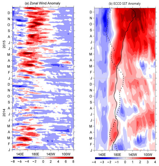
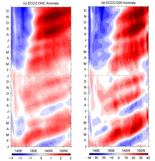
Figure 1.
Time-longitude plots of (a) Zonal surface wind anomalies (m/s); (b) ECCO SST anomalies (°C); (c) OHC anomalies (1 × 10⁻⁹ J/m2); and (d) 20 °C isotherm depth anomalies (m) averaged in the equatorial band (5° S–5° N) for the 2014–2015 warming event. Note: In the figure, the solid black line indicates the 29 °C isotherm of the 2014–2015 warming event; the Dotted black line shows that of the composite average; Plotted contour intervals were 2 m/s, 0.5 °C, 0.25 × 10⁻⁹ J/m2, and 5 m, respectively.
There were abruptly no more strong westerly wind anomalies observed during the following summer of 2014. However, three large easterly wind stress anomalies became strengthened from May to July. The easterly anomalies in May were confined to the equatorial western Pacific (Figure 1a), while the two in June and July spread across the entire equatorial Pacific region. This was possibly related to the colder SST anomalies of the subtropical southeastern Pacific [70]. The easterly wind anomalies strengthened the equatorial upwelling through Ekman transport and pushed the eastern edge of the warm pool back westward. The combined effects caused an abrupt decrease in the SST during the summer of 2014, as shown in Figure 1b.
In the following August to October period, several weak and short-duration westerly wind anomalies occurred again in the eastern-central Pacific region. These anomalies excited the eastward propagation of downwelling Kelvin waves but with weaker magnitudes. The eastern edge of the warm pool was not clearly further shifted eastward due to the weak westerly wind anomalies (Figure 1b). Furthermore, the weaker downwelling Kelvin waves resulted in a weak warm SST anomaly in the equatorial eastern-central Pacific by the year-end of 2014. This study found that the variability of the El Niño 3.4 index for the 1997–1998, 2015–2016 and Average show gradually increased for year 0 and declined in year 1. However, for 2014–2015, the index showed an upward trend, and it was much weaker compared to that of the composite El Niño in late 2014 (Figure 2a). The OHC anomaly also showed that the 2014–2015 event is very different from the other El Nino events (Figure 2b).
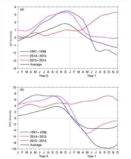
Figure 2.
(a) Time series analysis of the SST anomalies (°C) averaged over the El Niño 3.4 area; and (b) heat content anomalies (1 × 10⁻⁹ J/m2) in the equatorial Pacific band (5° S–5° N, 120° E–80° W) for each calendar month. Note: In the figure, the black line indicates the composite average El Niño; the Green line indicates the 1997–1998 El Niño; the Red line indicates the 2014–2015 warming event; and the cyan line indicates the 2015–2016 El Niño; The x-axis is marked with the calendar month from year 0 to the subsequent year 1.
In the period ranging from January to May of 2015, a series of westerly wind anomalies occurred. This once again pushed the western equatorial Pacific warm pool eastward, initiated the eastward propagation of equatorial downwelling Kelvin waves, and produced SST warming in the central-eastern Pacific. These dynamic characteristics were similar to those exhibited during early 2014. The major differences between the 2014 and 2015 atmospheric forces were the magnitude and position of the easterly wind anomalies in the equatorial Pacific in the month of June. The easterly wind anomalies in June of 2015 were much smaller in magnitude and shorter in duration. The weak maximum center was confined to the equatorial western Pacific and had almost disappeared in the central region when compared to that observed in June 2014 (Figure 1a). Consequently, the weaker easterly wind anomalies resulted in the upwelling Kelvin waves with smaller magnitudes that only slightly pushed the eastern edge of the western equatorial Pacific warm pool back westward. However, in the following winter months, another series of strong westerly anomalies were generated along the equator that maintained SST warming through similar dynamical impacts. Finally, a strong El Niño event occurred in the equatorial Pacific resulting in the development of extended and long-term warming trends at the end of 2015. Those trends were comparable in magnitude to the famed 1997–1998 El Niño event, as illustrated in Figure 2a.
3.2. Heat Budget of the Upper 300 m over the El Niño 3.4 Region
In order to analyze the different warming phases for the extended and long-term warming 2014–2015 event, time-longitude diagrams of the heat content tendency, averaged in the equatorial tropical Pacific band (5° S–5° N), was completed, as shown in Figure 3. It can be clearly seen in the figure that heat tendency was positive during the development phase of the 1997–1998 event and the composite average El Niño in the equatorial eastern Pacific (Figure 3b,c). Meanwhile, for the 2014–2015 warming event, the heat tendency was positive in the first three months (marked as the first phase warming) and then switched to negative values after the larger westerly anomalies burst in March (Figure 3d). The heat content tendency initially began to decrease and then increased after easterly anomalies occurred in June and July. Then, from July to the end of 2014, the heat content tendency of the band average was consistently positive, beginning the second warm-up phase with weaker magnitudes. Subsequently, from the beginning of 2015, the heat content tendency for the 2014–2015 event substantially increased. For the composite and the 1997–1998 El Niño events, the heat content tendency was characterized by negative values from autumn 0 to autumn 1, which became increasingly favorable conditions for La Nina to develop.
Figure 3.
Time-longitude plots of heat content tendency for (a) 2014–2015; (b) 1997–1998; (c) Composite tendency averaged in the equatorial tropical Pacific (5° S–5° N); (d) Variability of the averaged tendency (J/m2/s) given as a function of time.
In the present investigation, to identify the processes responsible for the different warming phases for the extended 2014–2015 warming event, a heat budget analysis was performed over the El Niño 3.4 area (Figure 4). The budget terms of the U and V (zonal and meridional) advection and subsurface processes of the 2014–2015 warming event were compared with those of the composite El Niño (Figure 5).
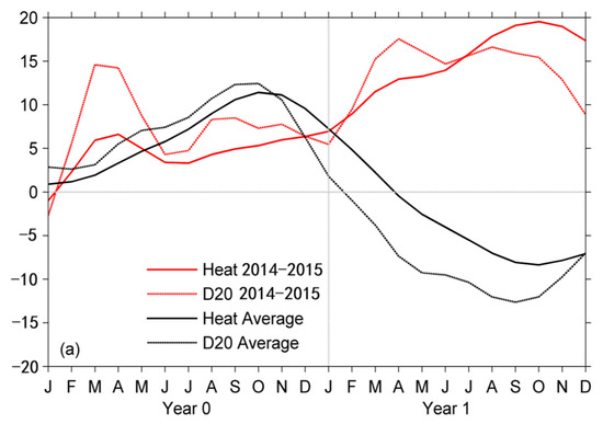
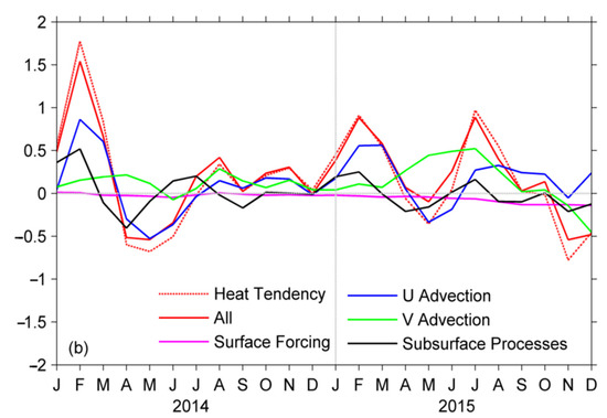
Figure 4.
(a) Time series of heat content anomalies (1 × 10⁸ J/m2); (b) Heat budget analysis (1 × 10¹⁵ J/s) in the El Niño 3.4 area. Note: In the figure, All = Surface forcing + U Advection + V Advection + Subsurface processes.
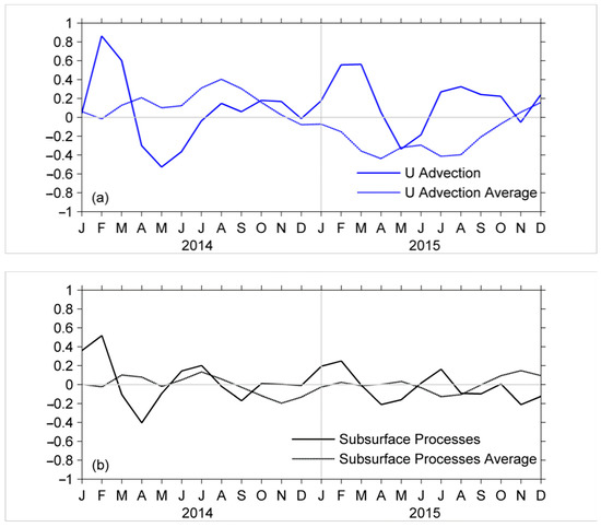
Figure 5.
Heat budget terms (1 × 10¹⁵ J/s) for (a) U Advection; (b) Subsurface processes; and (c) V Advection and comparison between the 2014–2015 warming and composite average El Niño.
Based on the time series analysis results of the heat content anomalies averaged over the El Niño 3.4 area (Figure 4a), it was determined that the heat content anomalies were significantly related to the 20 °C isotherm depth anomalies (D20) that had been revealed in the results of prior studies [71,72,73,74]. The results shown in Figure 4b suggested that the heat content tendency in the El Niño 3.4 area was largely dominated by U advection, subsurface processes, and V advection, while the impact of surface force was negligible. However, all four together explained nearly all of the OHC tendency, with a correlation coefficient (CC) above 0.985. The variations in the U advection were in phase with the OHC tendency, with their CC equal to 0.796.
At the beginning of the year 2014, the westerly wind anomalies in the equator region (Figure 1a) caused changes in the anomalous eastward velocity (Figure 6a). The surface currents expanded the warm pool eastward and increased the OHC in the central-western equatorial Pacific. Therefore, the U advection played a dominant role at the beginning of the warming phase. The largest amplitude reached 0.86 × 10¹⁵ J/s in February of that year (Figure 4b and Table 1) and accounted for 55.8% of the total OHC tendency. On the other hand, the downwelling equatorial Kelvin waves that had been triggered by the westerly wind anomalies deepened the thermocline and suppressed the normal cold water upwelling. Therefore, the subsurface processes were another important factor (33.8%) for the increased OHC. As a result of those two physical dynamical processes in the spring of 2014, the heat tendency was clearly positive in the first three months (Figure 4b). After larger westerly anomalies burst in March, no more westerly wind anomalies were observed, and easterly wind anomalies abruptly occurred in the following months of May, June, and July. Those easterly wind anomalies induced anomalous westward velocity and were favorable for equatorial Kelvin wave upwelling (Figure 6c). The OHC tendency then switched to negative values, reaching the strongest negative level (−0.54 × 10¹⁵ J/s) in May.
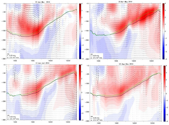
Figure 6.
Temperature anomalies with contour intervals of 0.2 °C; ocean zonal velocity anomalies; and vertical velocity (vectors), averaged within the equator band (5° N to 5° S) for the first year of the 2014–2015 warming event, results showed every three months. Note: In the figure, the black and green curves indicate the D20 and the climatology of the D20 averaged during the corresponding month, respectively.

Table 1.
OHC budget terms for the 2014–2015 warming event and the composite El Niño unit is 1 × 10¹⁵ J/s.
The analysis results indicated that those easterly wind anomalies played a major role in halting the development of the 2014–2015 warming event, which was found to be in agreement with the results of previous research [43,44]. For the composite average and the 1997–1998 El Niño, the OHC tendency was always positive in the equatorial western Pacific during the development process (Figure 3b,c). This was attributed to the contributions of the U advection, V advection, and subsurface processes, which were positive for the composite average El Niño (Figure 5).
After the halting of the summer warming phase, the OHC tendency began to increase. Then, the OHC turned to positive values from July to the end of 2014 due to the weaker westerly wind anomalies (Figure 1a). As is shown in Figure 4b, the U advection and V advection processes were positive and in the same order of magnitude. However, the subsurface processes were negligible (Figure 5b), and there were much weaker eastward propagating downwelling Kelvin waves (Figure 6d). Therefore, the wind anomalies were weaker and of shorter duration compared to those in the first three months of 2014 (Figure 1a). For the composite average El Niño, the U advection, V advection, and subsurface processes were negative, which tended to slow down the warming development speed in the winter of year 0 (Figure 5).
At the beginning of 2015, the U advection processes contributed to the ocean heat increasing to the highest degree. The most significant increase in the U advection processes was from to (Figure 5a) due to the gradual enhancement of the westerly wind anomalies (Figure 1a). These eastward propagation of the downwelling Kelvin waves also became stronger compared to that at the end of 2014 (Figure 7a,b). As a result, the subsurface processes gradually increased from approximately zero to (Figure 5b). The weaker easterly wind anomalies with shorter durations that occurred in the middle of 2015 resulted in negative U advection processes, with the least value reaching (compared to in the middle of 2014). Although the negative U advection and subsurface processes damped the development of the warming phase, it should be noted that the V advection processes were always positive during the 2014–2015 warming period, rapidly increasing from approximately at the beginning of 2015 to a maximum value of approximately in July of that year (Figure 5c). A leading role in the positive heat tendency was played by the V advection processes in the middle of 2015, after which another series of strong westerly anomalies occurred, and the U advection processes contributed to the extended 2014–2015 warming event.
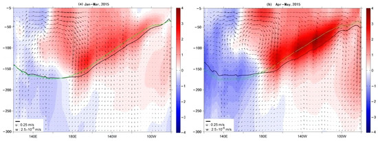
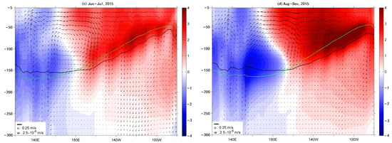
Figure 7.
Same as Figure 6, but for the second year of the 2014–2015 warming event, results showed every three months. Note: In the figure, the black and green curves indicate the D20 and the climatology of the D20 averaged during the corresponding month, respectively.
From August 2014 to October 2015, the OHC tendency was almost consistently positive, with the exception of a small negative value of in May 2015. The obvious increase in the OHC with time can be seen in Figure 4. It should be noted that the OHC anomalies reached more than at the beginning of 2015, exceeding the ordinary value (<) for composite average El Niño, as detailed in Figure 4a. This indicated that the stored OHC of 2014 gave the 2015–2016 El Niño warming event an important start and pushed El Niño to the level of an extreme warming event. Similar conclusions have also been suggested in previous studies [45,46].
4. Conclusions
In this study, results from the ECCO ocean datasets provided all of the terms of the heat budgets required to analyze the dynamic processes responsible for the extended 2014–2015 warming event. A budget analysis of the upper OHC over the upper 300 m was completed. The El Niño 3.4 SST anomalies index was employed as the indicator of El Niño in the present study. The data of seven El Niño events were obtained for the period ranging from 1993 to 2016. Then, a composite analysis was carried out to analyze the spatiotemporal characteristics, and the results were compared with the extended 2014–2015 warming event. Two scatterometers, QuikSCAT and ASCAT, were utilized to describe and analyze the zonal surface wind anomalies. The significant differences observed between the year 2014 and the year 2015 were the magnitudes and positions of the easterly wind anomalies in the equatorial Pacific during the month of June. The abrupt easterly wind anomalies of 2014 that spread over the entire equatorial Pacific triggered the upwelling of the equatorial Kelvin waves and pushed the eastern edge of the western equatorial Pacific warm pool back westward. This resulted in an abrupt decrease in the SST in the summer of 2014. In comparison, the easterly wind anomalies in 2015 were characterized by weaker magnitudes and shorter durations. These were limited to the western equatorial Pacific and had only minorly damped the increasing SST. After some westerly anomalies occurred in the winter of 2015, the SST continued its warming trend, and an extreme El Niño event developed.
Due to the differences in the SST warming characteristics in 2014 and 2015, a heat budget of the upper 300 m over the El Niño 3.4 region was performed to investigate the dynamical processes responsible for the different warming phases. It was determined that the heat content tendency was mainly controlled by the U advection processes, subsurface processes, and V advection processes. At the beginning of the warming phase in 2014, the U advection processes played a dominant role, accounting for more than half of the total ocean heat content tendency. The subsurface processes accounted for approximately one-third of the heat tendency. The western anomalous zonal advection processes largely caused a negative tendency due to the abrupt easterly wind anomalies that halted the development of the 2014–2015 warming phase. It was found that after the development of the summer warming trend had stopped, both the U advection and V advection processes contributed to the positive tendency in the latter half of 2014, with approximately the same weaker order of magnitude. For the warming phase of 2015, the heat tendency was controlled by similar dynamical processes when compared to that of 2014. The main difference was the occurrence of weaker easterly wind anomalies in the middle of 2015. The U advection and subsurface processes were negative during that period. However, the V advection processes played a leading role in the positive heat tendency, which indicated that there were different dynamical processes at play during the 2014 and 2015 easterly wind anomaly periods.
Author Contributions
Conceptualization, Y.Q.; Methodology, L.W. and H.M.; Software, Y.W.; Validation, Y.Q., H.M., Y.L. and Q.Y.; Writing—original draft preparation, Y.Q.; Writing—review and editing, X.W.; Project administration, L.W. All authors have read and agreed to the published version of the manuscript.
Funding
This research was funded by the National Basic Research Program of China (Grant number 2021YFC3101504), the National Natural Science Foundation of China (Grant numbers 42176030 and 41406042), and the China Scholarship Council (Grant number 201604180005).
Institutional Review Board Statement
Not applicable.
Informed Consent Statement
Not applicable.
Data Availability Statement
The ECCO ocean reanalysis, accessed on 15 March 2018, is available free of charge from http://ecco.jpl.nasa.gov/external/.
Acknowledgments
I would like to thank the China Scholarship Council for providing me with an opportunity to carry out research at the University of California, Los Angeles (UCLA) as a visiting scholar. We also would like to thank UCLA for providing the workspace to conduct our research. A special thanks to the research fellows of UCLA for valuable discussions.
Conflicts of Interest
The authors declare no conflict of interest.
References
- Ermakova, T.S.; Koval, A.V.; Smyshlyaev, S.P.; Didenko, K.A.; Aniskina, O.G.; Savenkova, E.N.; Vinokurova, E.V. Manifestations of different El Niño types in the dynamics of the extratropical stratosphere. Atmosphere 2022, 13, 2111. [Google Scholar] [CrossRef]
- Lee, T.; McPhaden, M.J. Increasing intensity of El Niño in the central equatorial Pacific. Geophys. Res. Lett. 2010, 37, L14603. [Google Scholar] [CrossRef]
- Kao, H.Y.; Yu, J.Y. Contrasting eastern-Pacific and central-Pacific types of ENSO. J. Clim. 2009, 22, 615–632. [Google Scholar] [CrossRef]
- Yeh, S.W.; Kug, J.S.; Dewitte, B.; Kwon, M.H.; Kirtman, B.P.; Jin, F.F. El Niño in a changing climate. Nature 2009, 461, 511–514. [Google Scholar] [CrossRef]
- Kug, J.S.; Jin, F.F.; An, S.I. Two types of El Niño events: Cold tongue El Niño and warm pool El Niño. J. Clim. 2009, 22, 1499–1515. [Google Scholar] [CrossRef]
- Ashok, K.; Behera, S.K.; Rao, S.A.; Weng, H.; Yamagata, T. El Niño Modoki and its possible teleconnection. J. Geophys. Res. 2007, 112, C11007. [Google Scholar] [CrossRef]
- Larkin, N.K.; Harrison, D.E. On the definition of El Niño and associated seasonal average U.S. weather anomalies. Geophys. Res. Lett. 2005, 32, L13705. [Google Scholar] [CrossRef]
- Wang, D.X.; Qin, Y.H.; Xiao, X.J.; Zhang, Z.Q.; Wu, X.Y. El Niño and El Niño Modoki variability based on a new ocean reanalysis. Ocean Dyn. 2012, 62, 1311–1322. [Google Scholar] [CrossRef]
- Yin, H.; Wu, Z.; Fowler, H.J.; Blenkinsop, S.; He, H.; Li, Y. The combined impacts of ENSO and IOD on global seasonal droughts. Atmosphere 2022, 13, 1673. [Google Scholar] [CrossRef]
- Pacheco, J.; Solera, A.; Avilés, A.; Tonón, M.D. Influence of ENSO on droughts and vegetation in a high mountain equatorial climate basin. Atmosphere 2023, 13, 2123. [Google Scholar] [CrossRef]
- Lv, A.; Fan, L.; Zhang, W. Impact of ENSO events on droughts in China. Atmosphere 2022, 13, 1764. [Google Scholar] [CrossRef]
- Ashok, K.; Yamagata, T. The El Niño with a difference. Nature 2009, 461, 481–484. [Google Scholar] [CrossRef] [PubMed]
- Kim, H.M.; Webster, P.J.; Curry, J.A. Impact of shifting patterns of Pacific Ocean warming on north Atlantic tropical cyclones. Science 2009, 325, 77–80. [Google Scholar] [CrossRef]
- Chang, C.W.J.; Hsu, H.H.; Wu, C.R.; Sheu, W.J. Interannual mode of sea level in the South China Sea and the roles of El Niño and El Niño Modoki. Geophys. Res. Lett. 2008, 35, L03601. [Google Scholar] [CrossRef]
- Chu, P.C. Global upper ocean heat content and climate variability. Ocean Dynam. 2011, 61, 1189–1204. [Google Scholar] [CrossRef]
- Paek, H.; Yu, J.Y.; Qian, C. Why were the 2015/2016 and 1997/1998 extreme El Niños different? Geophys. Res. Lett. 2017, 44, 1848–1856. [Google Scholar] [CrossRef]
- Fedorov, A.V.; Hu, S.; Lengaigne, M.; Guilyardi, E. The impact of westerly wind bursts and ocean initial state on the development, and diversity of El Niño events. Clim. Dyn. 2014, 44, 1381–1401. [Google Scholar] [CrossRef]
- Hu, S.; Fedorov, A.V.; Lengaigne, M.; Guilyardi, E. The impact of westerly wind bursts on the diversity and predictability of El Niño events: An ocean energetics perspective. Geophys. Res. Lett. 2014, 41, 4654–4663. [Google Scholar] [CrossRef]
- Chen, D.; Lian, T.; Fu, C.; Cane, M.A.; Tang, Y.; Murtugudde, R.; Song, X.S.; Wu, Q.Y.; Zhou, L. Strong influence of westerly wind bursts on El Niño diversity. Nat. Geosci. 2015, 8, 339–345. [Google Scholar] [CrossRef]
- Bjerknes, J. 1969. Atmospheric teleconnections from the equatorial Pacific. Mon. Weather Rev. 1969, 97, 163–172. [Google Scholar] [CrossRef]
- Cane, M.A.; Zebiak, S.E. A theory for El Niño and the Southern Oscillation. Science 1985, 228, 1085–1087. [Google Scholar] [CrossRef]
- Suarez, M.J.; Schopf, P.S. A delayed oscillator for ENSO. J. Atmos. Sci. 1988, 45, 3283–3287. [Google Scholar] [CrossRef]
- Picaut, J.; Ioualalen, M.; Menkes, C.; Delcroix, T.; McPhaden, M.J. Mechanism of zonal displacements of the Pacific Warm Pool: Implications of ENSO. Science 1996, 274, 1486–1489. [Google Scholar] [CrossRef] [PubMed]
- Jin, F.F. An equatorial ocean recharge paradigm for ENSO. Part I: Conceptual mdel. J. Atmos. Sci. 1997, 54, 811–829. [Google Scholar] [CrossRef]
- Jin, F.F. An equatorial ocean recharge paradigm for ENSO. Part II: A Stripped-down coupled model. J. Atmos. Sci. 1997, 54, 830–847. [Google Scholar] [CrossRef]
- Weisberg, R.H.; Wang, C. A western Pacific oscillator paradigm for the El Niño-Southern Oscillation. Geophys. Res. Lett. 1997, 24, 779–782. [Google Scholar] [CrossRef]
- Battisti, D.S.; Hirst, A.C. Interannual variability in a tropical atmosphere-ocean model: Influence of the basic state, ocean geometry and nonlinearity. J. Atmos. Sci. 1989, 46, 1687–1712. [Google Scholar] [CrossRef]
- Anderson, D.L.T.; Satachik, E.S.; Webster, P.B. The TOGA decade—Reviewing the progress of El Niño research and predictions. J. Geophys. Res. 1998, 103, 015602. [Google Scholar]
- McPhaden, M.J. Genesis and Evolution of the 1997-98 El Niño. Science 1999, 283, 950–954. [Google Scholar] [CrossRef]
- Chen, D.; Cane, M.A.; Kaplan, A.; Zebiak, S.E.; Huang, D. Predictability of El Niño over the past 148 years. Nature 2004, 428, 733–736. [Google Scholar] [CrossRef]
- Qu, T.; Yu, J.Y. ENSO Indices from Sea Surface Salinity Observed by Aquarius and Argo. J. Oceanogr. 2014, 70, 367–375. [Google Scholar] [CrossRef]
- Jin, E.K.; Kinter, J.L.; Wang, B.; Park, C.K.; Kang, I.S.; Kirtman, B.P.; Kug, J.S.; Kumar, A.; Luo, J.J.; Schemm, J.; et al. Current status of ENSO prediction skill in coupled ocean-atmosphere models. Clim. Dyn. 2008, 31, 647–664. [Google Scholar] [CrossRef]
- Moore, A.M.; Kleeman, R. Stochastic forcing of ENSO by the intraseasonal oscillation. J. Clim. 1999, 12, 1199–1220. [Google Scholar] [CrossRef]
- Wu, X.; Han, G.; Zhang, S.; Liu, Z. A study of the impact of parameter optimization on enso predictability with an intermediate coupled model. Clim. Dyn. 2016, 46, 711–727. [Google Scholar] [CrossRef]
- Latif, M.; Barnett, T.P.; Cane, M.A.; Flügel, M.; Graham, N.E.; Von Storch, H.; Xu, J.S.; Zebiak, S.E. A review of ENSO prediction studies. Clim. Dyn. 1994, 9, 167–179. [Google Scholar] [CrossRef]
- Webster, P.J. The annual cycle and the predictability of the tropical coupled ocean-athomosphere system. Meteorol. Atmos. Phys. 1995, 56, 33–55. [Google Scholar] [CrossRef]
- Goddard, L.; Mason, S.J.; Zebiak, S.E.; Ropelewski, C.F.; Basher, R.; Cane, M.A. Current approaches to seasonal-to-interannual climate predictions. Int. J. Climatol. 2001, 21, 1111–1152. [Google Scholar] [CrossRef]
- Ludescher, J.; Gozolchiani, A.; Bogachev, M.I.; Bunde, A.; Havlin, S.; Schellnhuber, H.J. Improved El Niño forecasting by cooperativity detection. Proc. Natl. Acad. Sci. USA 2013, 110, 11742–11745. [Google Scholar] [CrossRef]
- Penland, C.; Sardeshmukh, P.D. The optimal growth of tropical sea surface temperature anomalies. J. Clim. 1995, 8, 1999–2024. [Google Scholar] [CrossRef]
- Mcphaden, M.J. Playing hide and seek with El Niño. Nat. Clim. Chang. 2015, 5, 791–795. [Google Scholar] [CrossRef]
- Chen, S.; Wu, R.; Chen, W.; Yu, B.; Cao, X. Genesis of westerly wind bursts over the equatorial western pacific during the onset of the strong 2015–2016 El Niño. Atmos. Sci. Lett. 2016, 17, 384–391. [Google Scholar] [CrossRef]
- Li, J.; Liu, B.; Li, J.; Mao, J. A comparative study on the dominant factors responsible for the weaker-than-expected El Niño event in 2014. Adv. Atmos. Sci. 2015, 32, 1381–1390. [Google Scholar] [CrossRef]
- Min, Q.; Su, J.; Zhang, R.; Rong, X. What hindered the El Niño pattern in 2014? Geophys. Res. Lett. 2015, 42, 6762–6770. [Google Scholar] [CrossRef]
- Hu, S.; Fedorov, A.V. Exceptionally strong easterly wind burst stalling El Niño of 2014. Proc. Natl. Acad. Sci. USA 2016, 113, 2005–2010. [Google Scholar] [CrossRef] [PubMed]
- Bond, N.A.; Cronin, M.F.; Freeland, H.; Mantua, N. Causes and impacts of the 2014 warm anomaly in the NE Pacific. Geophys. Res. Lett. 2015, 42, 3414–3420. [Google Scholar] [CrossRef]
- Levine, A.F.Z.; McPhaden, M.J. How the July 2014 easterly wind burst gave the 2015–2016 El Niño a head start. Geophys. Res. Lett. 2016, 43, 6503–6510. [Google Scholar] [CrossRef]
- Hu, S.; Fedorov, A.V. The extreme El Niño of 2015–2016: The role of westerly and easterly wind bursts, and preconditioning by the failed 2014 event. Clim. Dyn. 2019, 52, 7339–7357. [Google Scholar] [CrossRef]
- Xue, Y.; Kumar, A. Evolution of the 2015/16 El Niño and historical perspective since 1979. Sci. China Earth Sci. 2017, 60, 1572–1588. [Google Scholar] [CrossRef]
- Hu, S.; Fedorov, A.V. The extreme El Niño of 2015–2016 and the end of global warming hiatus. Geophys. Res. Lett. 2017, 44, 3816–3824. [Google Scholar] [CrossRef]
- Santoso, A.; Mcphaden, M.J.; Cai, W. The defining characteristics of ENSO extremes and the strong 2015/2016 El Niño. Rev. Geophys. 2017, 55, 1079–1129. [Google Scholar] [CrossRef]
- Wyrtki, K. Water displacements in the Pacific and the genesis of El Niño cycles. J. Geophys. Res. 1985, 90, 7129–7132. [Google Scholar] [CrossRef]
- Cane, M.A.; Zebiak, S.E.; Dolan, S.C. Experimental forecasts of El Niño. Nature 1986, 321, 827–832. [Google Scholar] [CrossRef]
- Meinen, C.S.; McPhaden, M.J. Observations of warm water volume changes in the equatorial Pacific and their relationship to El Niño and La Nina. J. Clim. 2000, 13, 3551–3559. [Google Scholar] [CrossRef]
- Mcphaden, M.J. A 21st century shift in the relationship between ENSO SST and warm water volume anomalies. Geophys. Res. Lett. 2012, 39, L09706. [Google Scholar] [CrossRef]
- Ji, M.; Behringer, D.W.; Leetmaa, A. An improved coupled model for ENSO prediction and implications for ocean initialization. Part II: The coupled model. Mon. Wea. Rev. 1998, 126, 1022–1034. [Google Scholar] [CrossRef]
- Clarke, A.J.; Van Gorder, S. Improving El Niño prediction using a space-time integration of Indo-Pacific winds and equatorial Pacific upper ocean heat content. Geophys. Res. Lett. 2003, 30, 1399. [Google Scholar] [CrossRef]
- Xue, Y.; Balmaseda, M.A.; Boyer, T.; Ferry, T.N.; Good, S.; Ishikawa, I.; Kumar, A.; Rienecker, M.; Rosati, T.; Yin, Y. A Comparative Analysis of Upper-Ocean Heat Content Variability from an Ensemble of Operational Ocean Reanalyses. J. Clim. 2012, 25, 6905–6929. [Google Scholar] [CrossRef]
- Gao, S.; Qu, T.; Nie, X. Mixed layer salinity budget in the tropical Pacific Ocean estimated by a global GCM. J. Geophys. Res. Oceans 2014, 119, 8255–8270. [Google Scholar] [CrossRef]
- Fukumori, I. A partitioned Kalman filter and smoother. Mon. Weather Rev. 2002, 130, 1370–1383. [Google Scholar] [CrossRef]
- Qu, T.; Gao, S.; Fukumori, I. What governs the sea surface salinity maximum in the North Atlantic? Geophys. Res. Lett. 2011, 38, L07602. [Google Scholar] [CrossRef]
- Kim, S.B.; Fukumori, I.; Lee, T. The closure of the ocean mixed layer temperature budget using level-coordinate model fields. J. Atmos. Ocean. Technol. 2006, 23, 840–853. [Google Scholar] [CrossRef]
- Kim, S.B.; Lee, T.; Fukumori, I. Mechanisms controlling the interannual variation of mixed layer temperature averaged over the Nino-3 region. J. Clim. 2007, 20, 3822–3843. [Google Scholar] [CrossRef]
- Kalnay, E.; Kanamitsu, M.; Kistler, R.; Collins, W.; Deaven, D.; Gandin, L.; Iredell, M.; Saha, S.; White, G.; Woollen, J.; et al. The NCEP/NCAR 40-year reanalysis project. Bull. Am. Meteor. Soc. 1996, 77, 437–472. [Google Scholar] [CrossRef]
- Reynolds, R.W.; Smith, T.M. Improved global sea-surface temperature analyses using optimum interpolation. J. Clim. 1994, 7, 929–948. [Google Scholar] [CrossRef]
- Barnier, B.; Siefridt, L.; Marchesiello, P. Thermal forcing for a global ocean circulation model using a three-year climatology of ECMWF analysis. J. Mar. Syst. 1995, 6, 363–380. [Google Scholar] [CrossRef]
- Large, W.G.; McWilliams, J.C.; Doney, S.C. Oceanic vertical mixing: A review and a model with a nonlocal boundary layer parameterization. Rev. Geophys. 1994, 32, 363–403. [Google Scholar] [CrossRef]
- Lee, T.; Fukumori, I.; Tang, B. Temperature advection: Internal versus external processes. J. Phys. Oceanogr. 2004, 34, 1936–1944. [Google Scholar] [CrossRef]
- Zhang, X.; Mcphaden, M.J. Surface layer heat balance in the eastern equatorial pacific ocean on interannual time scales: Influence of local versus remote wind forcing. J. Clim. 2010, 23, 4375–4394. [Google Scholar] [CrossRef]
- Gent, P.R.; McWilliams, J.C. Isopycnal mixing in ocean circulation models. J. Phys. Oceanogr. 1990, 20, 150–155. [Google Scholar] [CrossRef]
- Zhu, J.S.; Kumar, A.; Huang, B.H.; Balmaseda, M.A.; Hu, Z.Z.; Marx, L.; Kinter, J.L. The role of off-equatorial surface temperature anomalies in the 2014 El Niño prediction. Sci. Rep. 2016, 6, 19677. [Google Scholar] [CrossRef]
- Rebert, J.P.; Donguy, J.R.; Eldin, G.; Wyrtki, K. Relations between sea level, thermocline depth, heat content, and dynamic height in the tropical pacific ocean. J. Geophys. Res. 1985, 90, 11719. [Google Scholar] [CrossRef]
- Wen, C.; Kumar, A.; Xue, Y.; Mcphaden, M.J. Changes in tropical pacific thermocline depth and their relationship to enso after 1999. J. Clim. 2014, 27, 7230–7249. [Google Scholar] [CrossRef]
- Xu, K.; Huang, R.X.; Wang, W.; Zhu, C.; Lu, R. Thermocline fluctuations in the equatorial pacific related to the two types of El Niño events. J. Clim. 2017, 30, 6611–6627. [Google Scholar] [CrossRef]
- Zhu, J.; Kumar, A.; Huang, B. The relationship between thermocline depth and SST anomalies in the eastern equatorial Pacific: Seasonality and decadal variations. Geophys. Res. Lett. 2015, 42, 4507–4515. [Google Scholar] [CrossRef]
Disclaimer/Publisher’s Note: The statements, opinions and data contained in all publications are solely those of the individual author(s) and contributor(s) and not of MDPI and/or the editor(s). MDPI and/or the editor(s) disclaim responsibility for any injury to people or property resulting from any ideas, methods, instructions or products referred to in the content. |
© 2023 by the authors. Licensee MDPI, Basel, Switzerland. This article is an open access article distributed under the terms and conditions of the Creative Commons Attribution (CC BY) license (https://creativecommons.org/licenses/by/4.0/).