The Impacts of the Application of the Ensemble Optimal Interpolation Method in Global Ocean Wave Data Assimilation

Abstract

The ensemble optimal interpolation method was used in this study to conduct an examination of the assimilations of significant wave height (SWH) data from HY-2A satellite altimeter based on the WAVEWATCH III global ocean wave model. The results suggested that the ensemble optimal interpolation method using HY-2A SWH data played a positive role in enhancing the accuracy of the global ocean wave simulations and could effectively improve the deviations of SWH in the simulation processes. The root mean square errors of the NDBC buoy inspections were improved by 7 to 44% after the assimilation, and those of China’s offshore buoy inspections were improved by 3 to 11% after the assimilation. It was observed that the farther the buoys were from the shore, the better the effects of the assimilation improvements. The root mean square errors of the Jason-2 satellite data validations were improved by 17% after the assimilation, with monthly improvements of 8–25%. The improvements occurred in most of the global oceans, particularly in the Southern Ocean, the Eastern Pacific Ocean and the Indian Ocean. The results obtained in this research can be used as a reference for the operational applications of China’s ocean satellite data in ocean wave data assimilation and prediction.

1. Introduction

Ocean waves are sea surface fluctuation phenomena caused by winds and are major dynamic processes in the upper ocean layers that are considered to play an important role in regulating the upper ocean turbulent mixing [1]. Ocean waves are also key elements of the global climate system, and wave modeling on global scales is of much importance in ocean climate studies [2]. The damages caused by ocean waves are important components of marine disasters. Ocean waves are the most important disaster-causing factors leading to human death or disappearance among various marine disasters, and they seriously affect the safety of marine development and production. The development of offshore structures requires attention to ocean wave information, and significant wave loads become crucial design factors [3]. In recent years, numerical predictions of ocean waves have received close attention due to the scarcity of observational data and the importance of ocean waves. In short-term ocean wave numerical predictions, the accuracy of the initial fields cannot be ignored. It has been found that data assimilation technology is a relatively cost-effective method for the improvement of initial field predictions and the analysis of historical data.

With the vast improvement in temporal and spatial coverage of the ocean provided by satellite observations, ocean phenomena can be observed and understood more comprehensively [4]. Large quantities of near real-time ocean wave observation data have been obtained in recent years due to the rapid development of ocean satellite remote sensing technology. Guaranteed reliable data have been made available for conducting research using ocean wave assimilation technology. The international community began studies of the applications of ocean wave data assimilations in the 1980s. In the 1990s, altimeter significant wave height (SWH) data assimilation technology was successfully applied to operational applications. The methods used in ocean wave assimilations included the gradual correction method [5,6]; optimal interpolation (OI) method [7,8,9,10,11,12,13]; variational method [14,15,16,17,18]; and the Kalman filter method [19,20], among which the most commonly used were OI and the variational method. The background error covariance of OI was derived from empirical formulae, which was not sufficient to describe the true status of the background errors. Evensen [21] proposed the ensemble Kalman filter (EnKF) method, which combined ensemble predictions with the Kalman filter using the Monte Carlo principle. The operations of the models were driven by disturbance initial fields, and the background errors were estimated by forming multiple sets of ensemble samples through multiple sets of disturbance experiments. Since the background errors could be adjusted along with the integrating processes, it was possible to better characterize the variations of the errors over time and space. However, the computational complexity was enormous. Based on the OI method, Evensen [22] also proposed ensemble optimal interpolation (EnOI) as a suboptimal method of the EnKF. Similarly to the EnKF method, the EnOI method also uses ensemble samples to estimate the covariance of the model background errors. However, EnKF evaluates the model errors based on the ensemble prediction fields, and its errors change in real time with the integration of the model. EnOI replaces the sampled ensemble required by EnKF with static historical samples. Therefore, when compared with EnKF, the EnOI method only requires analysis of a specific sample, which has the advantages of requiring only small amounts of computing resources and low system maintenance costs. As a reliable and efficient assimilation method, EnOI has been widely used in ocean model assimilations, but there has been less research conducted for ocean wave assimilations. Cao et al. [23] applied the EnOI method to the assimilation of satellite altimeter SWH data in the South China Sea. It was found that the EnOI method could effectively improve the accuracy of the ocean wave simulations, indicating that the method had promising prospects in operational applications.

Currently, the satellite altimeter data commonly used in ocean wave assimilation research were mainly obtained from the ERS-1/2, Envisat series satellites [24,25,26]; Geosat satellite [8]; TOPEX, Jason-1/2/3 series satellites [11,23,27,28]; and the SARAL satellite [12,29]. In recent years, China independently launched the HY-2 series of satellites, which has changed the long-term dependence on foreign countries for satellite ocean wave data and provided large amounts of near real-time data for operational forecasting and verification processes. However, there has been relatively little research regarding the application of HY-2 satellite data to ocean wave assimilations. Wang et al. [30] carried out application studies using HY-2 satellite altimeter wave data to SWAN model data assimilation of typhoon “Lipee”. They found that the assimilation using HY-2 satellite altimeter wave data could improve the accuracy of the initial field and forecasting field.

In summary, as a reliable and efficient assimilation method, EnOI has not yet been attempted in global ocean wave assimilation, and there is also very little research on the application of China’s HY-2 satellite data in ocean wave data assimilation. The National Marine Environmental Forecasting Center of China established a global ocean wave operational prediction system based on the WAVEWATCH III Model. In this study, based on the WAVEWATCH III global ocean wave model, an assimilation study of SWH data from the HY-2A satellite altimeter was conducted using the EnOI method. The applicability of the assimilation method in global ocean wave simulations was quantitatively evaluated. The results obtained in this study also provide references for the operational applications of Chinese ocean satellite data in ocean wave assimilation and prediction processes.

This paper is organized as follows: Section 1 includes the introduction; Section 2 describes the wave model and data; Section 3 describes the EnOI assimilation method; Section 4 presents the analysis of the assimilation results; Section 5 includes the discussions; and Section 6 provides the conclusions.

2. Wave Model and Data

The operational wave numerical prediction model WAVEWATCH III of the National Marine Environmental Forecasting Center of China was used in this study. The WAVEWATCH III ocean wave model is a third-generation numerical ocean wave model developed by the National Centers for Environmental Prediction (NCEP) of the National Oceanic and Atmospheric Administration (NOAA) of the United States [31]. The WAVEWATCH III model adopts a physical process different from that used by other third-generation ocean wave models. It utilizes a highly accurate third-order difference scheme in its numerical predictions and has developed a spatial averaging method to solve GSE effects. WAVEWATCH III uses the wave action density spectrum in the control equation, that is, $N(k,\theta )\equiv F(k,\theta )/\sigma$, where $k$ is the wave number, $\theta$ is the direction of wave propagation, and $\sigma =2\pi f$ is the natural frequency. Wave propagation is then described by $\frac{dN}{dt}=\frac{S}{\sigma }$, where $S$ represents the net source term. In deep water, the net source term $S$ is generally considered to consist of a wind–wave interaction term $S_{in}$, a nonlinear wave-wave interaction term $S_{nl}$ and a dissipation (“whitecapping”) term $S_{ds}$. In shallow water, it is also necessary to consider wave–bottom interactions $S_{bot}$ [31]. Currently, WAVEWATCH III is being used in multiple operational centers, such as the United States NCEP, British Weather Service, and the Korean Weather Service.

The calculation area of the model was located at 78° S–78° N, 0–360°. The southern and northern boundary conditions were zero, and the east–west periodic boundary conditions were used. The spatial resolution of the model was 1/3° × 1/3°. In the two-dimensional spectral space of frequency and direction, the initial frequency of the spectrum was 0.04118 Hz, which was divided into 25 frequency bands. The relationship between each frequency band was fⁿ⁺¹ =1.1 × fⁿ (n = 0, 1,…, 24). The wave directions were divided into uniform grids, with a total of 24 directions and a resolution of 15°. The maximum global time step and maximum CFL time step for x-y and k-theta were all 450 s, and the minimum source term time step was 300 s. The general bathymetric chart of the oceans (GEBCO) 30″ grid data were applied as the terrain data. The NCEP reanalysis wind field was used as the forced wind field with spatial and temporal resolutions of 0.5° × 0.5° and six hours, respectively.

This study used the orbital SWH data of the HY-2A satellite altimeter as the assimilation data. The HY-2A satellite is the first marine dynamic environment satellite independently launched by China. It integrates active and passive microwave remote sensors and is capable of high-precision orbital measurements and determinations, as well as 24/7 all-weather global detection. Its main mission is to monitor and investigate marine environments and obtain various marine dynamic environment parameters, including sea surface wind fields, wave heights, ocean currents, and sea surface temperatures. Remote sensing loads include microwave scatterometers, radar altimeters, and microwave radiometers. The HY-2A satellite orbit is a solar synchronous orbit with an orbital height of 971 km, an inclination angle of 99.34° and a repetition period of 14 days. Some scholars have conducted studies on error comparison and correction of the SWH data between HY-2A satellites and other satellites. Chen et al. [32] evaluated HY-2A SWH data in the South China Sea using NDBC buoy data and Jason-1/2 altimeter data and corrected HY-2A data using the linear regression method. It was found that the root mean square error (RMSE) of HY-2A SWH data compared with NDBC buoy was 0.36 m, which was close to Jason-1/2 (0.35 m and 0.37 m, respectively). After calibration, the RMSE of the HY-2A data was 0.27 m, while that of Jason-1/2 was 0.27 m and 0.23 m, respectively. Xu et al. [33] also used NDBC buoy data and Jason-1/2 altimeter data to evaluate the SWH data of HY-2A and calibrate the HY-2A data following the method used by Queffeulou [34]. They found that there was a significant linear relationship between HY-2A SWH data and Jason-1/2 altimeter data, with correlation coefficients generally greater than 0.95. It indicated that HY-2A SWH data can accurately reflect the state of the ocean.

The orbital SWH data from the Jason-2 satellite altimeter and the NDBC buoy data, as well as China’s offshore buoy data, were used in this study for validation purposes. The Jason-2 satellite was jointly developed by the Centre National d’Études Spatiales (CNES), the National Aeronautics and Space Administration (NASA), the European Organization for the Exploration of Meteorological Satellites (EUMETSAT) and the National Oceanic and Atmospheric Administration (NOAA) of the United States. The orbit altitude of the Jason-2 satellite was 1336 km, the inclination angle was 66.039°, and the repetition period was 9.9156 days. The NDBC buoy data were derived from the National Data Buoy Center (NDBC) of the NOAA (http://www.ndbc.noaa.gov/, accessed on 19 September 2022). It can provide standard meteorological output data, continuous wind data, one-dimensional spectral data of ocean waves, and so on. The data on China’s offshore buoys were obtained from the Marine Early Warning and Monitoring Department of the Ministry of Natural Resources of China. The elements observed included wind speeds, wind directions, temperature levels, atmospheric pressure levels, relative humidity, water temperatures, average wave heights, average wave periods, significant wave heights, significant wave periods, one-tenth wave heights, one-tenth wave periods, maximum wave heights, maximum wave periods, and so on. The buoy position accuracy was 0.01′, and the accuracy of the SWH data was 0.1 m. The positions of the NDBC buoys and China’s offshore buoys are shown in Figure 1.

3. Assimilation Method

EnOI is based on OI, with the latter determining the background errors through empirical formulae, and the former using ensemble samples to estimate the background error covariance of the model. During the integration process of the model, only a static sample that does not change over time needs to be analyzed. The analytical equations for the EnOI assimilation method are as follows [22]:

$$X_a=X_b+W(d-H{X}_b)$$

(1)

$$W={P{H}^T(HP{H}^T+R)}^{-1},P=\frac{\mathsf{\alpha }{A}^{\prime }{A^{\prime }}^T}{N-1}$$

(2)

where Xa is the SWH analysis field; X_b is the SWH background field; W denotes the gain matrix; d indicates the observation field; H is the observation operator; P represents the background error covariance matrix; R is the observation error covariance matrix; and α represents the weight assigned to the background error covariance field. In the EnOI assimilation experiment conducted in this study, α was set to 1; A indicates an ensemble sample; N denotes the number of ensemble sample members; $\overline{A}$ indicates the ensemble average and ensemble perturbation $A^{\prime }=A-\overline{A}$; and T denotes transposition.

The final analysis equation of the EnOI method was obtained as follows [22]:

$$X_a=X_b+\alpha A^{\prime }{A^{\prime }}^T{H}^T{(\alpha H{A}^{\prime }{A^{\prime }}^T{H}^T+\left(N-1\right)R)}^{-1}(\mathrm{d}-\mathrm{H}{X}_b)$$

(3)

In this study, the assimilation data were extracted from the HY-2A SWH data. Therefore, the observation errors of the altimeter had to be considered during the assimilations. It was believed that the observation errors of the HY-2A SWH data conformed to a Gaussian distribution with a mean value of 0, and there was no significant correlation between the observation errors at different positions. The observation error covariance matrix R was represented by the diagonal matrix $R_{ij}={\sigma }_o^2{\delta }_{ij}$, where ${\sigma }_o$ is the observation error; and ${\delta }_{ij}$ is the function of $i$ and $j$, when $i=j$ and ${\delta }_{ij}=1$ and when $i\ne j$ and ${\delta }_{ij}=0$, respectively. In accordance with the estimations of previous related research regarding the observation errors of SWH in the HY-2A data, the accuracy of the HY-2A SWH data has greatly improved since April 2013 (with an error of 0.3 m), making the accuracy level similar to that of the Jason-2 satellite’s SWH data [35]. Moreover, quality control was completed prior to the assimilation of the HY-2A data, including removing invalid data and SWH data that significantly exceed a reasonable range (>32 m). Multiple data retrieved from the satellite altimeter were mutually corrected. A horizontal consistency test was performed where a datum was removed if that datum was significantly different from the neighboring data. Finally, the outlier data were removed, and a linear regression correction was performed. The observation error ${\sigma }_o$ after quality control was set to 0.25 m. The assimilation time window was one hour (±30 min).

For the selection process of the ensemble samples, 100 samples were randomly selected from the same month within three years of the models’ integration as the ensemble samples for that month. To avoid any computational problems caused by a large number of observations, the sample covariance matrix of the model state vector was localized. The maximum distance from the observation point to the grid point (influence radius) was determined (taken as 1500 km in the EnOI assimilation experiment in this study), and it was assumed that only observations within the influence radius would affect the analysis of that grid point. Then, the observational data impacting that point were filtered out, and each grid point was analyzed and calculated.

The observation update (d$-$H$X_b)$ was weighted during the actual numerical implementation process to avoid significant discontinuity emerging after assimilations at the boundary between the assimilated and non-assimilated regions. This was expected to reflect that the closer the grid points were to the observation points, the greater the update effects were on the grid points during the assimilation process. However, the effects were actually observed to become gradually less impactful until the grid points exceeded the influence radius and were not affected by the assimilations whatsoever.

WAVEWATCH III is a full-spectrum spatial wave model that predicts ocean waves by calculating their spectra. Since the object in the assimilation module was the SWH, it was necessary to reconstruct new ocean wave spectra using the SWH analysis fields. In this study, the method used by Cao [23] was referenced, and different reconstruction formulae were adopted for wind waves and swells. Firstly, it was assessed whether the wave propagation direction $\theta$ and phase velocity $C_p$ conformed to $\frac{28\left|u_{\mathrm{*}}\right|}{C_p}\cos (\theta -{\theta }_w)<1$, where $u_{\mathrm{*}}$ indicates friction velocity and ${\theta }_w$ indicates wind direction. If they did, it was a swell; otherwise, it was a wind wave. Then, the following formulae were used to reconstruct the wind waves and swells [23]:

Wind wave:

$$F_{aij}\left(f,\theta \right)=a{F}_{bij}\left(f,\theta \right),a={(\frac{H_{aij}}{H_{bij}})}^2$$

(4)

Swell:

$$F_{aij}\left(f,\theta \right)=a{F}_{bij}\left(f+△f,\theta \right), △f=f_b-(\frac{f_b}{a^{1/4}})$$

(5)

where $F_{bij}$ and $F_{aij}$ are the wave spectra before and after reconstruction on the grid points (i, j); $H_{bij}$ and $H_{aij}$ are the significant wave heights before and after assimilation on the grid points (i, j), namely, the background field and the analysis field; and $f$ and $\theta$ are the wave frequency and direction.

4. Results

Two groups of experiments were conducted in this study, including a control experiment without assimilation and an assimilation experiment using the EnOI method to assimilate the HY-2A SWH data. The experiments were conducted throughout the year 2015. The selection of the ensemble samples and the setting of assimilation-related parameters are described in Section 3. The ocean wave data used for the validations were selected from the SWH data observed by NDBC, China’s offshore buoys, and Jason-2 altimeter satellite. Although the reliability of the buoy data was higher, the buoys were mainly located in the Atlantic and Pacific Oceans and China’s offshore regions, resulting in significant limitations. Therefore, the systematic validation process required the use of satellite altimeter data with wide coverage for comparisons across the globe. The validation statistics included deviation (Bias), RMSE, correlation coefficient (Corr), relative error (RE) and scatter index (SI), as represented by the following formulae:

$$Bias=\frac{1}{N}{\sum }_{i=1}^N(P_i-O_i)$$

(6)

$$RMSE=\sqrt{\frac{1}{N}{\sum }_{i=1}^N{(P_i-O_i)}^2}$$

(7)

$$Corr=\frac{{\sum }_{i=1}^N(P_i-\overline{P})(O_i-\overline{O})}{[{\sum }_{i=1}^N(P_i-\overline{P}{)}^2{\sum }_{i=1}^N(O_i-\overline{O}{)}^2{]}^{\raisebox{1ex}{$1$}\!\left/ \!\raisebox{-1ex}{$2$}\right.}}$$

(8)

$$RE=\frac{1}{N}{\sum }_{i=1}^N\left|\frac{P_i-O_i}{O_i}\right|$$

(9)

$$SI=\frac{\sqrt{\frac{1}{N}{\sum }_{i=1}^N{\left[\left(P_i-\overline{P}\right)-\left(O_i-\overline{O}\right)\right]}^2}}{\overline{O}}$$

(10)

where $P_i$ is the simulation value, $O_i$ is the observed value and $N$ is the number of samples.

4.1. Validations with NDBC Buoy Data

The test results were validated using SWH data from six NDBC buoys in 2015, including the South Pacific buoy 32012; the North Pacific buoy 46066; the North Atlantic buoys 41041, 41047 and 41048; and the Hawaii buoy 51002. The time interval for the buoy data was one hour. The buoy position distribution is shown in Figure 1a. The validation results are detailed in Figure 2 and

Table 1. The statistical parameters of the NDBC buoy validations.

NDBC	DATA	Bias (m)	RMSE (m)	RE (%)	SI (%)	Corr	Number
46066	WW3	0.09	0.56	13.4	19.5	0.93	8709
	ENOI	0.00	0.46	11.2	16.0	0.95
51002	WW3	0.35	0.45	18.1	20.3	0.89	7812
	ENOI	0.16	0.29	10.4	12.9	0.92
32012	WW3	0.30	0.39	16.4	18.0	0.92	8728
	ENOI	0.05	0.22	8.0	10.1	0.94
41041	WW3	0.07	0.20	7.6	10.0	0.94	8270
	ENOI	0.06	0.18	7.1	9.2	0.95
41047	WW3	−0.06	0.30	10.7	18.2	0.94	8718
	ENOI	−0.03	0.28	11.2	17.2	0.94
41048	WW3	−0.11	0.45	11.7	24.2	0.89	8708
	ENOI	−0.07	0.42	11.5	23.0	0.90

Abbreviations: Bias, deviation; RMSE, root mean square error; RE, relative error; SI, scatter index; Corr, correlation coefficient.

. It was found that the EnOI assimilation scheme used in this study had significantly improved the simulations of the ocean waves at the six buoy positions. The average deviations were all closer to zero and the RMSEs were also significantly reduced after assimilation. The validated RMSE of buoy 32012 was improved by 44% after assimilation. The ocean waves at that buoy were mainly swells propagated from the westerlies of the southern hemisphere. The RMSEs of the other buoy validations were improved by 7–36% after assimilation. Therefore, the results indicated that the adoption of the EnOI method to assimilate HY-2A SWH data had played a positive role in improving the accuracy of the ocean wave simulations.

4.2. Validations with the Chinese Offshore Buoy Data

The SWH data from five offshore buoys in China were gathered in this study to analyze the test results. The position distributions of the buoys are shown in Figure 1b, and the validation results are shown in Figure 3. It was found that although the selected buoy positions were relatively close to the shore, the assimilations still played a positive role in improving the accuracy of the ocean wave simulations. Various statistical indicators were improved, and the simulations of some larger waves after assimilation were closer to the observations.

Table 2. The statistical parameters of China’s offshore buoy validations.

BUOY	DATA	Bias (m)	RMSE (m)	RE (%)	SI (%)	Corr	Number
1	WW3	0.15	0.31	16.68	22.28	0.92	6962
	ENOI	0.15	0.30	15.36	21.78	0.92
2	WW3	0.13	0.31	14.37	20.43	0.93	7885
	ENOI	0.12	0.29	13.33	19.73	0.93
3	WW3	0.02	0.35	16.77	26.68	0.87	7546
	ENOI	0.02	0.34	16.25	25.90	0.88
4	WW3	0.15	0.37	16.04	20.66	0.94	8277
	ENOI	0.14	0.36	15.29	20.21	0.94
5	WW3	0.26	0.44	19.20	22.98	0.93	6191
	ENOI	0.23	0.39	16.83	20.49	0.94

lists the statistical parameters for the five buoy validations, where the RMSEs were improved by 3–11% after assimilation. The improvement effects of the assimilations were not obvious near the shoreline. However, the farther away the buoys were from the shore, the better the effects of the assimilations. The main reason for this may lie in the fact that the accuracy of the HY-2A SWH data tends to be low in places with shallow water near shorelines.

4.3. Validations Using Altimeter

This study’s test results were evaluated using the orbital SWH data of the Jason-2 satellite altimeter in 2015. The overall reliability of the two groups of test results was quantitatively analyzed in comparison with the Jason-2 SWH data. Figure 4 shows the monthly error values calculated using the Jason-2 satellite SWH data. It was found that the positive deviation of the model simulations had improved after the assimilations, reducing the model’s overestimations of the significant wave heights. In addition, the RMSEs, relative errors, scatter indexes and correlation coefficients also showed varying degrees of improvement in each month after the assimilations. For example, the RMSEs had improved by 8 to 25% each month and 17% on average throughout the year. The relative errors had improved by 16 to 30%, with an average improvement of 24% throughout the year. Overall, the application of the EnOI method to ocean wave assimilations yielded satisfactory results.

The global deviation distributions of the model results are displayed in Figure 5. Figure 5a presents the deviation distributions of the control experiment results. We can observe that there was a significant negative deviation in the Northwest Atlantic Ocean and a strong positive deviation in most other sea areas, especially in the Southern Ocean and the Pacific Ocean. This was consistent with the inspection results of the NDBC buoys. As indicated above, the deviations of the WAVEWATCH III model could be effectively improved by assimilating HY-2A orbital SWH data. From Figure 5b, we can easily see that after EnOI assimilation, the global deviations were significantly decreased, and the improvements occurred in most of the global oceans, particularly in the ocean areas with relatively high deviations, such as the Southern Ocean and the Pacific Ocean.

Figure 6 shows the global RMSEs of the control run and EnOI assimilation run. As displayed in Figure 6a, relatively high RMSEs could be found in the Southern Ocean, the North Pacific and the North Atlantic. General improvements in RMSEs could be found globally in Figure 6b, particularly with significant reductions in the Southern Ocean and the Eastern Pacific Ocean, which prove the positive impact of data assimilation.

To quantitatively evaluate the global pattern of the RMSE improvements after assimilation, we calculated the differences between Figure 6a,b, as shown in Figure 7. The color red represents positive improvements, while the color blue represents negative improvements after assimilation. It could be seen that after EnOI assimilation by using the HY-2A SWH data, the RMSEs of SWH simulations in the vast majority of the global ocean decreased, especially in the Southern Ocean, the Eastern Pacific Ocean and the Indian Ocean. However, we could also observe a few cases of deterioration in the nearshore areas on the east coast of the mainland, such as the Bohai Sea in China and eastern Florida in the United States. Ocean waves in these areas were mainly offshore waves caused by local winds with poor response to assimilation, which could be the reason for this. There were also more cyclone activities in these areas. In addition, the accuracy of the satellite data tended to reduce when approaching the nearshore.

5. Discussions

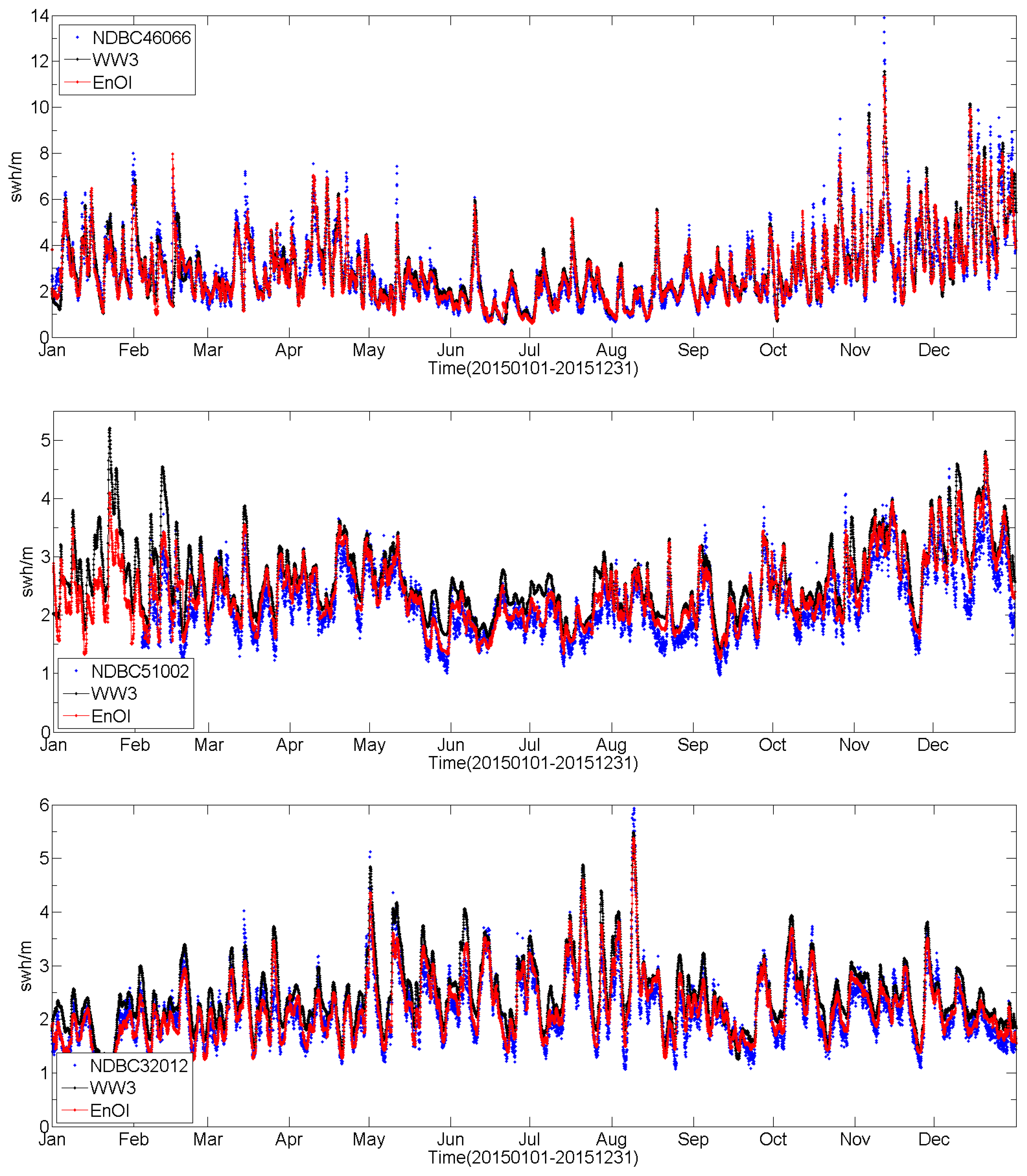
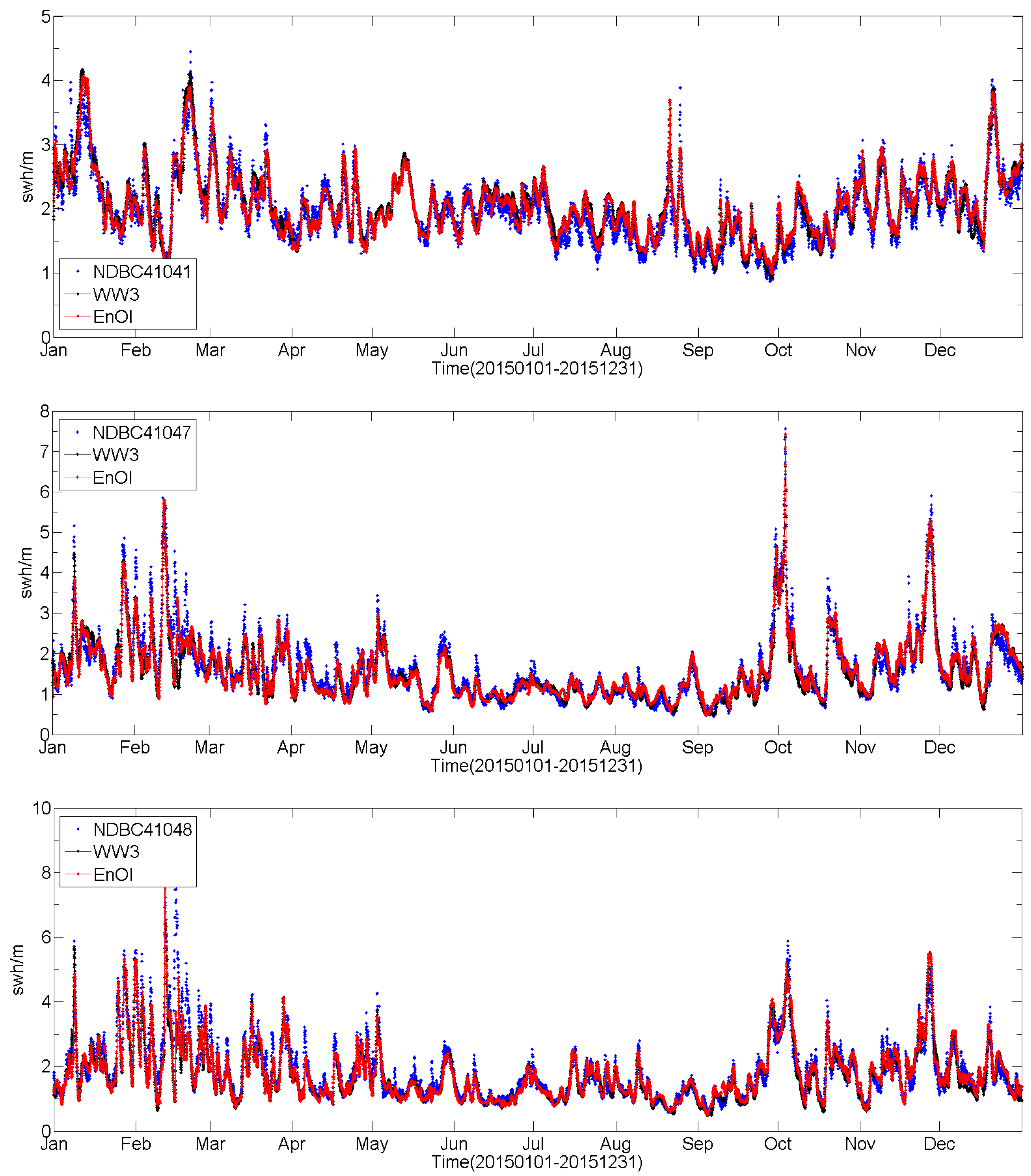
In this study, an EnOI global ocean wave assimilation system was constructed based on the WAVEWATCH III ocean wave model. An analysis of the assimilations of SWH data from the HY-2A satellite altimeter was conducted. The assimilation results were evaluated using the NDBC data, Chinese offshore buoy data and Jason-2 satellite data.

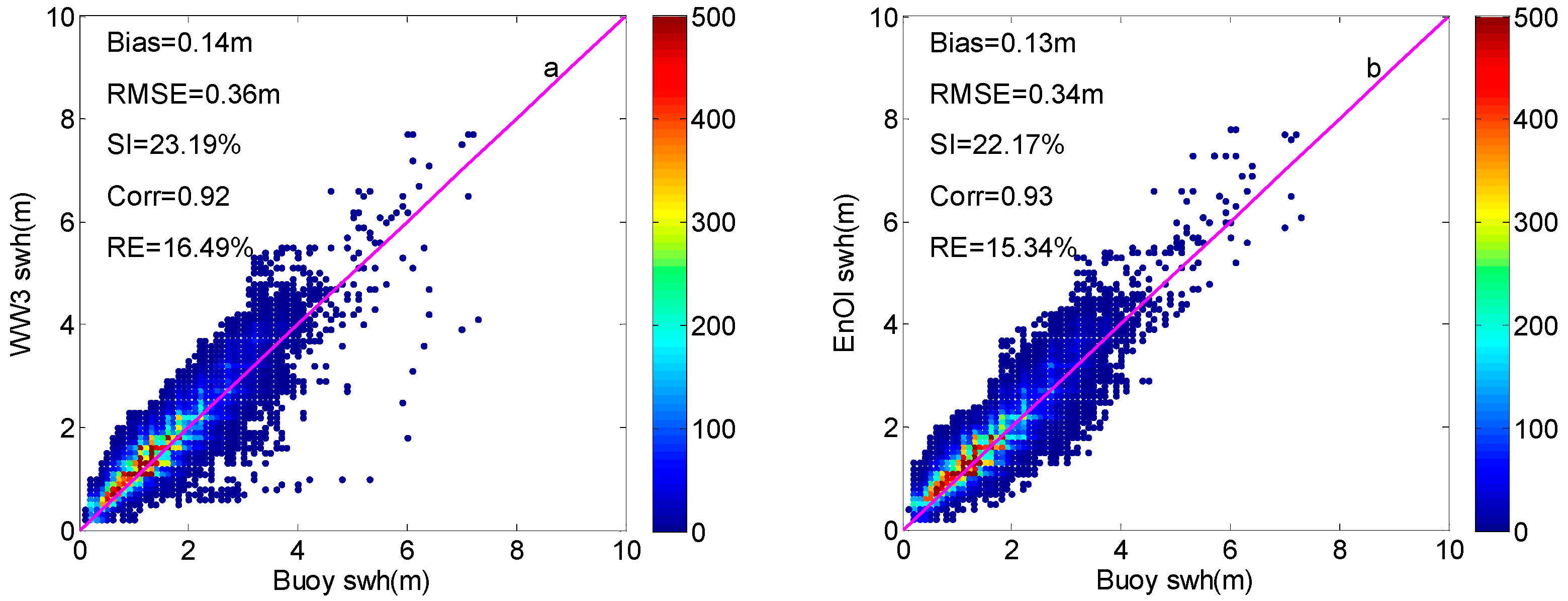
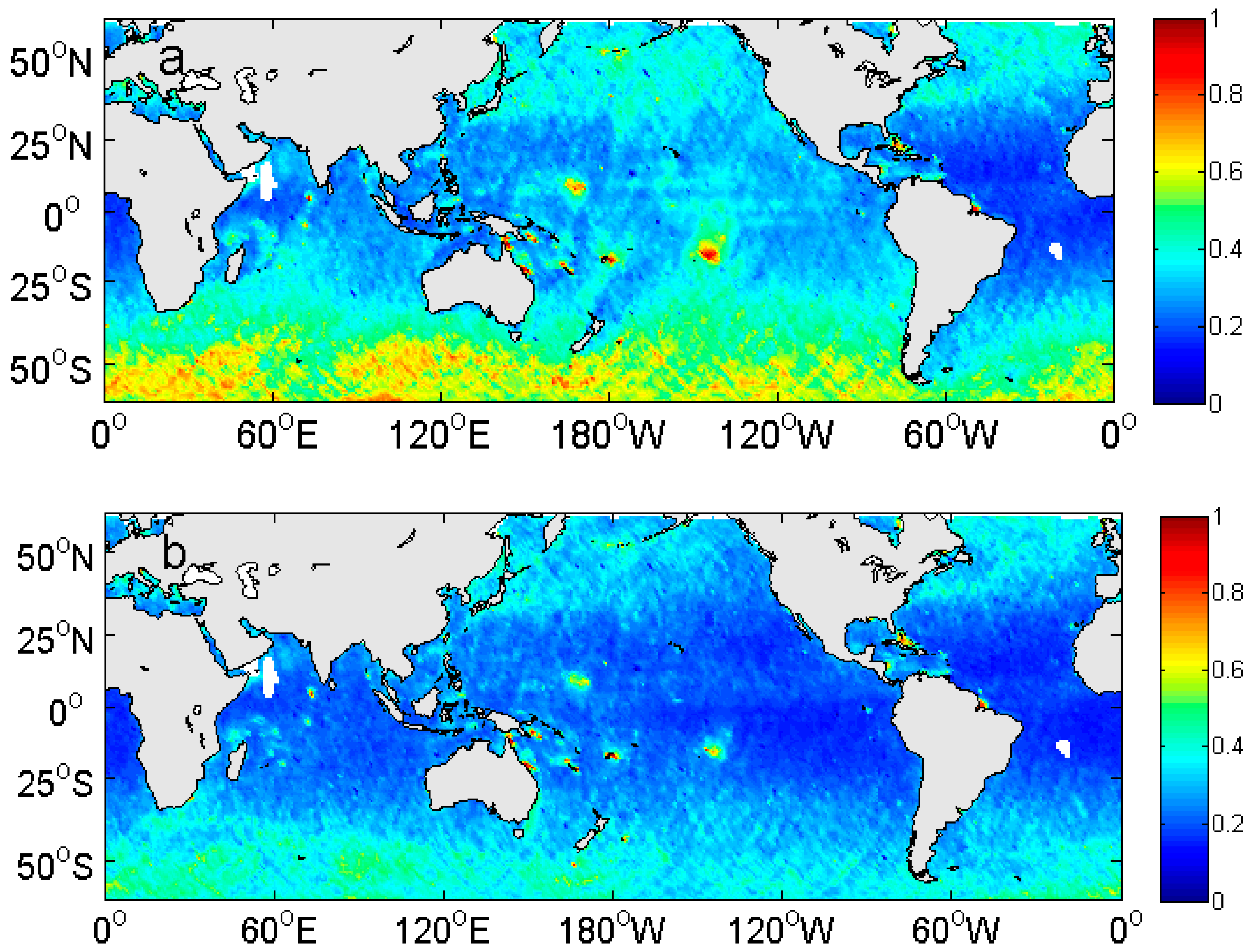
The assimilations of the HY-2A SWH data using the EnOI method played a positive role in improving the accuracy of the global ocean wave simulations and effectively improved the deviations in the SWH simulations. The RMSEs of the NDBC buoy validations were improved by 7 to 44% following the assimilations, and those of the Chinese offshore buoy validations were improved by 3 to 11%. The improvement effects of the assimilations were not obvious near the shoreline. However, the farther the distance the buoys were from the shoreline, the better the assimilation effects. The main reason for this may be that the accuracy of the HY-2A SWH data tends to be reduced in shallow-water shoreline regions. The RMSEs of the Jason-2 satellite data validations were improved by 17% after assimilation, with 8 to 25% improvements each month. The improvements had mainly occurred in the global oceans, particularly in the Southern Ocean, the Eastern Pacific Ocean and the Indian Ocean.

6. Conclusions

Based on the WAVEWATCH III global ocean wave model, the assimilation effect of the EnOI method using SWH data from HY-2A was analyzed and evaluated. It was found that the results obtained using the EnOI and HY-2A data for global ocean wave assimilation were encouraging, which effectively improved the positive deviations of the model simulations and alleviated the overestimations of SWH by the model. Various statistical indicators showed varying degrees of improvement. The EnOI method only needs to integrate a specific sample with a low computational cost. As a reliable and efficient assimilation method, EnOI can be considered for operational application in global wave assimilation. The results obtained in this study also provide references for the operational applications of Chinese ocean satellite data in ocean wave assimilation.

This study has not yet researched the impact of the EnOI assimilation method on the global ocean wave prediction stage. In the next step, the assimilation method used in this study will be applied to conduct assimilation research by using the HY-2B/2C and CFOSAT satellite data on the ocean wave analysis and prediction stages, with the goal of comprehensively mastering the applications of China’s ocean satellite data in global ocean wave simulations and predictions.

References

1. Zhang, W.; Li, R.; Zhu, D.; Zhao, D.; Guan, C. An investigation of impacts of surface waves-induced mixing on the upper ocean under typhoon Megi (2010). Remote Sens. 2023, 15, 1862. [Google Scholar] [CrossRef]
2. Tavekoli, S.; Khojasteh, D.; Haghani, M.; Hirdaris, S. A review on the progress and research direction of ocean engineering. Ocean Eng. 2023, 272, 113617. [Google Scholar] [CrossRef]
3. Amaechi, C.V.; Reda, A.; Butler, H.O.; Ja’e, I.A.; An, C. Review on fixed and floating offshore structures. Part II: Sustainable design approaches and project management. J. Mar. Sci. Eng 2022, 10, 973. [Google Scholar] [CrossRef]
4. Li, X.; Han, G.; Yang, J.; Wang, C. Remote sensing analysis of typhoon-induced storm surges and sea surface cooling in Chinese coastal waters. Remote Sens. 2023, 15, 1844. [Google Scholar] [CrossRef]
5. Breivik, L.A.; Reistad, M. Assimilation of ERS-1 altimeter wave heights in an operational numerical wave model. Weather Forecast. 1994, 9, 440–451. [Google Scholar] [CrossRef]
6. Breivik, L.A.; Reistad, M.; Schyberg, H.; Sunde, J.; Krogstad, H.E.; Johnsen, H. Assimilation of ERS SAR wave spectra in an operational wave model. J. Geophys. Res. 1998, 103, 7887–7900. [Google Scholar] [CrossRef]
7. Thomas, J.P. Retrieval of energy spectra from measured data for assimilation into a wave model. Q. J. R. Meteorol. Soc. 1988, 114, 781–800. [Google Scholar] [CrossRef]
8. Lionello, P.; Günther, H.; Janssen, P.A.E.M. Assimilation of altimeter data in a global third-generation wave model. J. Geophys. Res. 1992, 97, 14453–14474. [Google Scholar] [CrossRef]
9. Young, I.R.; Glowacki, T.J. Assimilation of altimeter wave height data into a spectral wave model using statistical interpolation. Ocean Eng. 1996, 23, 667–689. [Google Scholar] [CrossRef]
10. Greenslade, D.J.M. The assimilation of ERS-2 significant wave height data in the Australian region. J. Mar. Syst. 2001, 28, 141–160. [Google Scholar] [CrossRef]
11. Wang, Y.; Yu, Z. Validation of impact of assimilation of altimeter satellite significant wave height on wave forecast in the northwest Pacific. Acta Oceanol. Sin. 2009, 31, 1–8. [Google Scholar] [CrossRef]
12. Aouf, L.; Lefèvre, J.M. On the impact of the assimilation of SARAL/AltiKa wave data in the operational wave model MFWAM. Mar. Geod. 2015, 38 (Suppl. S1), 381–395. [Google Scholar] [CrossRef]
13. Smit, P.B.; Houghton, I.A.; Jordanova, K.; Portwood, T.; Shapiro, E.; Clark, D.; Sosa, M.; Janssen, T.T. Assimilation of significant wave height from distributed ocean wave sensors. Ocean Model. 2021, 159, 101738. [Google Scholar] [CrossRef]
14. Heras, D.L.M.; Burgers, G.; Janssen, P.A.E.M. Variational wave data assimilation in a third generation wave model. J. Atmos. Ocean. Technol. 1994, 11, 1305–1369. [Google Scholar]
15. Heras, D.L.M.; Burgers, G.; Janssen, P.A.E.M. Wave data assimilation in the WAM wave model. J. Mar. Syst. 1995, 6, 77–85. [Google Scholar] [CrossRef]
16. Bauer, E.; Hasselmann, K.; Young, I.R. Assimilation of wave data into the wave model WAM using an impulse response function method. J. Geophys. Res. 1996, 101, 3801–3816. [Google Scholar] [CrossRef]
17. Song, Q.; Mayerle, R. A 4D variational assimilation scheme with partition method for nearshore wave models. Ocean Dyn. 2017, 67, 989–1002. [Google Scholar] [CrossRef]
18. Song, Q.; Mayerle, R.; Yu, Y.; Li, C. An application study on adjoint-based variational wave assimilation scheme in German Bight with low spatial observation coverage. J. Oceanogr. 2020, 76, 29–41. [Google Scholar] [CrossRef]
19. Voorrips, A.C.; Heemink, A.W.; Komen, G.J. Wave data assimilation with the Kalman filter. J. Mar. Syst. 1999, 19, 267–291. [Google Scholar] [CrossRef]
20. Sun, M.; Yin, X.; Yang, Y.; Wu, K. An effective method based on dynamic sampling for data assimilation in a global wave model. Ocean Dyn. 2017, 67, 433–449. [Google Scholar] [CrossRef]
21. Evensen, G. Sequential data assimilation with a nonlinear quasigeostrophic model using Monte Carlo methods to forecast error statistics. J. Geophys. Res. 1994, 99, 10143–10162. [Google Scholar] [CrossRef]
22. Evensen, G. The Ensemble Kalman Filter: Theoretical formulation and practical implementation. Ocean Dyn. 2003, 53, 343–367. [Google Scholar] [CrossRef]
23. Cao, L.; Hou, Y.; Qi, P. Altimeter significant wave height data assimilation in the South China Sea using Ensemble Optimal Interpolation. Chin. J. Oceanol. Limnol. 2015, 33, 1309–1319. [Google Scholar] [CrossRef]
24. Hasselmann, S.; Lionello, P.; Hasselmann, K. An optimal interpolation scheme for the assimilation of spectral wave data. J. Geophys. Res. 1997, 102, 15823–15836. [Google Scholar] [CrossRef]
25. Skandrani, C.; Lefevre, J.M.; Queffeulou, P. Impact of multi-satellite altimeter data assimilation on wave analysis and forecast. Mar. Geod. 2004, 27, 511–533. [Google Scholar] [CrossRef]
26. Ren, Q.; Zhang, J.; Yin, X.; Yang, Y. Optimal interpolation assimilation experiments based on Envisat ASAR ocean wave spectral data. J. Trop. Oceangr. 2010, 29, 17–23. [Google Scholar]
27. Zhang, Z.; Qi, Y.; Shi, P.; Li, Z.; Li, Y. Application of an optimal interpolation method in South China Sea. J. Trop. Oceangr. 2003, 22, 34–41. [Google Scholar]
28. Sun, M.; Du, J.; Yang, Y.; Yin, X. Evaluation of Assimilation in the MASNUM Wave Model Based on Jason-3 and CFOSAT. Remote Sens. 2021, 13, 3833. [Google Scholar] [CrossRef]
29. Seemanth, M.; Remya, P.G.; Bhowmick, S.A.; Sharma, R.; Balakrishnan Nair, T.M.; Kumar, R.; Chakraborty, A. Implementation of altimeter data assimilation on a regional wave forecasting system and its impact on wave and swell surge forecast in the Indian Ocean. Ocean Eng. 2021, 237, 109585.1–109585.12. [Google Scholar] [CrossRef]
30. Wang, T.; Qi, L.; Zhu, J.; Wang, J.; Song, P.; Wang, X. Application studies of using HY-2 satellite altimeter wave data in ensemble optimal interpolation method-“Lipee” for instance. Acta Oceanol. Sin. 2017, 39, 29–38. [Google Scholar] [CrossRef]
31. Tolman, H.L. User manual and system documentation of WAVEWATCH IIITM version 3.14. Tech. Note NOAA/NWS/NCEP/MMAB 2009, 276, 194. [Google Scholar]
32. Chen, C.; Zhu, J.; Lin, M.; Zhao, Y.; Huang, X.; Wang, H.; Zhang, Y.; Peng, H. The validation of the significant wave height product of HY-2 altimeter–primary results. Acta Oceanol. Sin. 2013, 32, 82–86. [Google Scholar] [CrossRef]
33. Xu, G.; Yang, J.; Xu, Y.; Pan, Y.; Chen, X. Validation and calibration of significant wave height from HY-2 satellite altimeter. J. Remote Sens. 2014, 18, 206–214. [Google Scholar]
34. Queffeulou, P.; Croize, F.D. Global altimeter SWH data set. Biochem. Oral Biol. 2010, 100, 1–4. [Google Scholar]
35. Ye, X.; Lin, M.; Xu, Y. Validation of Chinese HY-2 satellite radar altimeter significant wave height. Acta Oceanol. Sin. 2015, 34, 60–67. [Google Scholar] [CrossRef]
Figure 1. Positions of the National Data Buoy Center (NDBC) buoys and China’s offshore buoys. (a) Positions of the NDBC buoys; (b) positions of China’s offshore buoys.
Atmosphere 14 00818 g001
Figure 2. Time series distributions of significant wave height (SWH) from model results and NDBC. The red dotted lines are the ensemble optimal interpolation (EnOI) assimilation test results; the black dotted lines are the control test results; the blue dots are buoy observations.
Atmosphere 14 00818 g002aAtmosphere 14 00818 g002b
Figure 3. The comparisons of SWH from model runs with China’s offshore buoy data. (a,b) The results of the control run and EnOI assimilation run. The magenta lines are the 1:1 lines, and the color bars indicate data volume.
Atmosphere 14 00818 g003
Figure 4. Statistical validations using the Jason-2 satellite’s SWH data.
Atmosphere 14 00818 g004
Figure 5. The deviation distributions of SWH from model runs in comparison with Jason-2. (a) Mapping of the control run; (b) mapping of the EnOI assimilation run.
Atmosphere 14 00818 g005
Figure 6. The distributions of the root mean square error of SWH from model runs in comparison with Jason-2. (a) Mapping of the control run; (b) mapping of the EnOI assimilation run.
Atmosphere 14 00818 g006
Figure 7. The distributions of the root mean square error improvements computed for the EnOI assimilation run in comparison with the control run.
Atmosphere 14 00818 g007