Article

Machine Learning for Fog-and-Low-Stratus Nowcasting from Meteosat SEVIRI Satellite Images

1
Direction Générale de la Météorologie, Direction des Systémes d’Observation/Centre National du Climat, Casablanca P.O. Box 8106, Morocco
2
Department of Hydraulics, Environment and Climate, Hassania School for Public Works, Casablanca P.O. Box 8108, Morocco
3
Institut Pierre-Simon Laplace, Institut de Recherche pour le Développement, 75252 Paris, France
*
Author to whom correspondence should be addressed.
Atmosphere 2023, 14(6), 953; https://doi.org/10.3390/atmos14060953
Submission received: 21 April 2023 / Revised: 17 May 2023 / Accepted: 28 May 2023 / Published: 30 May 2023
(This article belongs to the Special Issue Decision Support System for Fog)

Abstract

:
Fog and low stratus (FLS) are meteorological phenomena that have a significant impact on all ways of transportation and public safety. Due to their similarity, they are often grouped together as a single category when viewed from a satellite perspective. The early detection of these phenomena is crucial to reduce the negative effects that they can cause. This paper presents an image-based approach for the short-term nighttime forecasting of FLS during the next 5 h over Morocco, based on geostationary satellite observations (Meteosat SEVIRI). To achieve this, a dataset of hourly night microphysics RGB product was generated from native files covering the nighttime cold season (October to April) of the 5-year period (2016–2020). Two optical flow techniques (sparse and dense) and three deep learning techniques (CNN, Unet and ConvLSTM) were used, and the performance of the developed models was assessed using mean squared error (MSE) and structural similarity index measure (SSIM) metrics. Hourly observations from Meteorological Aviation Routine Weather Reports (METAR) over Morocco were used to qualitatively compare the FLS existence in METAR, where it is also shown by the RGB product. Results analysis show that deep learning techniques outperform the traditional optical flow method with SSIM and MSE of about 0.6 and 0.3, respectively. Deep learning techniques show promising results during the first three hours. However, their performance is highly dependent on the number of filters and the computing resources, while sparse optical flow is found to be very sensitive to mask definition on the target phenomenon.

1. Introduction

Poor visibility associated with fog and/or low stratus (FLS) affects many socio-economic sectors, such as aviation, marine, and road transportation [1,2,3,4,5,6,7]. This is why the monitoring of fog phenomenon has become a scientific topic of interest [8,9,10,11,12,13,14]. In recent years, with the rapid development of socio-economic sectors, fog detection and forecasting have become more and more important. Thus, the possibility of obtaining accurate hazardous weather warnings at least one or few hours in advance could help in the planning and mobilization of the responsible agencies and may contribute to reducing losses, mitigating damage and saving lives. Fog and low stratus are types of clouds consisting of water particles in liquid and/or solid forms that persist close to the earth’s surface. The main distinction between the two is their cloud base altitude, with fog touching the ground and low stratus forming above it. Despite this difference, they are often grouped together as a single category (FLS) when viewed from a satellite perspective [15]. On the other hand, FLS predictability is highly impacted by the lack of data in some regions, particularly on small-scale atmospheric features that affect FLS formation and dissipation. In some regions, such as rural areas or developing countries, these data may be limited or unavailable. In addition, the current weather observation network may not capture the variation in temperature and humidity in areas where FLS cover is lower and more prevalent, such as over urban areas [16,17] or mountainous regions [18]. This can make it difficult to produce accurate forecasts of FLS. In this framework, only remote-sensing systems can adequately provide high-resolution spatial coverage.
Different techniques have been proposed for short-term weather forecasting [19,20]. Traditional techniques used for nowcasting are highly parametric, hence complex, and these methods require long computation times when applied to large areas, which, added to the data reception time, often makes the first forecasts useless. Recently, there has been increasing interest towards the use of artificial intelligence techniques for weather nowcasting [21,22,23,24,25]. In weather forecasting, machine learning (ML) techniques are emerging as suitable tools that are expected to supplement major components of operational systems. In fact, the number of available machine learning tools continues to grow, particularly the open-source ones, due to the rising importance of artificial intelligence in today’s highly competitive business environment. Deep learning (DL) techniques continue to lead to breakthroughs in the fields of signal and image processing, especially for tasks such as image classification, object detection or image segmentation [26,27,28,29,30]. Thanks to their short execution times at inference, deep learning techniques are very attractive to nowcasting applications and thus are attracting the interest of operational meteorological centers.
In this work, we are interested in a particular family of deep neural networks that have been used extensively in satellite imagery studies, namely, convolutional neural networks (CNNs). Le Goff [31] compared CNN to other classical neural networks for cloud detection and terrain classification evaluated from a database of SPOT 6 album images, containing a large and representative variety of cloud coverage and landscapes. The performance is measured per pixel precision, and the results show that the performance of CNN is the best compared to that of other networks [31]. Zhang et al. [32] showed the good performance of CNN in fog detection and their capabilities in fully exploiting spatial and spectral information based on meteorological satellite data (Himawari-8 standard data, HSD8). In other subsequent works, the combination of the two architectures long short-term memory (LSTM) and CNN was made (ConvLSTM architecture), and it showed very satisfactory performance [33,34,35]. Tan et al. [36] proposed a model based on the ConvLSTM architecture to predict the future satellite clouds images using the infrared satellite images obtained by the FY-2F meteorological satellite of China. The developed model is designed to fuse multi-scale features in the hierarchical network structure to predict the pixel value and the morphological movement of the cloudage simultaneously. Guo et al. [37] proposed a deep learning model suitable for cloud detection, which is based on a U-Net network. This architecture uses a symmetric encoder–decoder structure, which is one of the most popular methods for semantic medical image segmentation. To train and test the proposed model, a dataset derived from the Landsat 8 satellite, which contains nine spectral bands is used. This model achieved good results in the cloud detection tasks, indicating that this symmetric network architecture has great potential for application in satellite image processing and deserves further research.
Cloud motion can be determined from sequential pictures obtained from sky cameras and satellite images [38] and one of the most prominent techniques for the tracking step is referred to as optical flow, which is a technique for deriving a velocity field from consecutive images. It is widely used in image analysis and has become increasingly popular in meteorological applications over the past 20 years [30,39,40]. This method was used in [41] as a technique for predicting cloud movement using ground-based sky imagery for use in short-term solar forecasting. It accurately tracked the movement of the clouds and predicted the trajectory using the Lucas–Kanade algorithm [42]. To forecast the movement, a linear regression through all the previous locations of each feature is applied. Results show that this algorithm is well suited to cloud tracking because the movement of clouds is small between images, and the longer the forecast, the larger the error present. Mondragon et al. [42] presented a model that predicts cloud advection displacement for different sky conditions and cloud types at the pixel level, using images obtained from a sky camera, as well as mathematical methods and the Lucas–Kanade method to measure optical flow. Zaher and Ghanem [43] also showed that optical flow algorithms have good accuracy for low motion, but this accuracy decreases significantly at high speeds. This is because moving objects do not preserve their intensity values from image to image in the case of high motions. For the majority of the analyzed events, models from the dense optical flow group outperform the operational baseline [44,45]. The sparse optical flow group of models showed significant skill, yet they generally performed more poorly than the dense optical flow group.
On a national scale, many studies have pointed out that the north-western part of Morocco is the most fog-prone area [8]. Concerning road traffic in this region, a fog event with minimum visibility below 200 m caused accidents in January 2011 that damaged about 50 vehicles and left a dozen injured [46]. With regard to air traffic, in January 2008, a fog event led to the diversion to other national airports of 21 aircraft that were supposed to land at the Mohammed V Airport, located in the target region [12]. These previous studies were conducted to better understand the physical mechanisms leading to FLS occurrence over the target area in each study. Other research studies have tried to improve the FLS forecasting, particularly at the main airports of Morocco. However, the operational NWP suffers from two main challenges: (1) taking advantage of the growing volume of data collected from satellites and other sources, and (2) satisfying the society’s increasing dependence on forecasts with ever-improving accuracy and reliability. Considered to be one of the suitable tools that will supplement major components of operational systems, many AI methods have been used in numerical modeling that aim to enhance the operational NWP model by replacing sub grid-scale parameterizations (e.g., [23]) or to build a full ML predictive model based on observation data and/or NWP forecasts (e.g., [19]). However, most of these research studies focused on a single site, often an airport. Recently, few AI-based studies have dealt with space and time dimensions in forecasting the reduced visibility phenomenon, such as fog and mist (e.g., [23]). Thus, more advanced studies are needed to push the frontiers of the FLS forecasting.
Hence, following the recent successes of DL techniques, we also leverage state-of-the-art image-to-image translation techniques in the field of remote sensing. To the best of our knowledge, the present paper is the first study to investigate the capability of deep learning approaches (classical CNNs, Unet, and convolutional LSTM networks (ConvLSTMs)) [47,48,49] for extracting spatial and temporal features from image sequences of Meteosat SEVIRI satellite data. This study also aims to obtain accurate and timely geostationary satellite image’s forecasts in the nowcasting framework over Morocco. From a geographical standpoint, FLS forecasting using deep learning algorithms over the North African regions has received little attention in the literature. In addition, this approach could be used in operation worldwide and would be of great benefit in areas where the observation stations are missing. The performance of these DL techniques will be assessed in comparison with a solid baseline consisting of the optical flow algorithm in its two flavors: dense and sparse.
This article is organized as follows. An overview on the FLS climatology over the study domain is detailed in Section 2.1. The used datasets (Meteosat SEVIRI satellite images data and synoptic stations observations) are described in Section 2.2. The principle of both versions (sparse and dense) of optical flow are introduced in Section 2.3. The DL techniques used in the modeling phase are briefly described in Section 2.4, where the formulation of the FLS nowcasting problem and the experimental design are also explained. The criteria of evaluation of the developed models are presented in Section 2.5. The main results are reported in Section 3. The discussion is contained in Section 4.

2. Materials and Methods

2.1. FLS Climatology over the Study Area

The study domain covers Morocco, which is located in the northwestern corner of Africa between latitudes 20.8° and 36° north and longitudes 1° and 17° west (Figure 1). Morocco is characterized by very different local climate types modulated by the orographic effects induced by the Atlas mountains [50,51]. Thus, we can find a large variety of climates ranging from moderate humid and sub-humid climates at the north of the High Atlas to semi-arid and arid climates in the south of the Atlas [52]). Many studies at the global, regional and national scales have pointed out that Morocco is one of the most vulnerable territories to climate change in the Mediterranean and North Africa (e.g., [53]). As a result, this could impact FLS occurrence over this region.
In Bari et al. [8], fog-type analysis shows that advection–radiation fog events are the most common fog type in the northwestern part of Morocco, followed by fog resulting from cloud-base lowering and radiation fog. Regarding the diurnal and seasonal distribution of the fog events, a maximum of their occurrence is classically observed during nighttime in winter. In addition, the synoptic analysis demonstrates that the advective processes associated with the sea-breeze circulation during daytime, followed by nocturnal radiational cooling early in the night, can often lead to fog formation over the northwestern part of Morocco. Morocco is generally characterized by a cold and moist northerly to northwesterly wind associated with the atmospheric perturbations coming from the American continent and also from the north of the Atlantic Ocean, resulting in the formation of stratiform low-level clouds over the ocean that extend inland over Morocco [54]. The low-level clouds also form near the upwelling zones due to the transportation of warm moist air from the seaward side of these zones. Cropper et al. [55] determined two zones that are interested by the upwelling occurrence: (a) 21–26 N with strong permanent annual upwelling zone; and (b) 26–35 N with weak permanent annual upwelling zone.
During the night (focus period of this study), Figure 2 shows the frequency distribution of the onset time of FLS events as a function of their duration over the 17 synoptic stations that are working 24 h/24 h from a total of 43 stations. This figure clearly points out that FLS event occurrences are frequent in the evening (18 UTC and 19 UTC) just after sunset and before sunrise (06 UTC). The local time is equal to the Greenwich mean time (GMT). In addition, we also note that the FLS events at the end of the night last longer. A noteworthy feature of the FLS climatology is that FLS events which do not last more than 3 h are the most frequent.

2.2. Datasets

The main goal of this research work is to elaborate a forecasted fog night microphysics RGB product that will be used by the forecaster for decision making regarding the FLS nowcasting. Indeed, the aim of using RGBs is to provide fast, easily understandable visual information. To achieve this goal, two datasets covering the cold season (October to April, the fog prone season) of 5 years (From 2016 to 2020), are used: (1) the hourly observations of visibility and low cloudiness, extracted from METARs of 43 synoptic meteorological stations (Figure 1), are used to compare qualitatively the FLS existence in METAR, where it is also shown by the satellite images, and (2) the High Rate SEVIRI Level 1.5 Image Data-MSG-0 degree from the Earth Observation Portal of EUMETSAT (https://eoportal.eumetsat.int/, accessed on 10 February 2021), extracted each hour in a native format that are used to develop the DL models. The MSG satellite’s main payload is the optical imaging radiometer, the so-called Spinning Enhanced Visible and Infrared Imager (SEVIRI) with its 12 spectral channels (4 visible/NIR and 8 IR channels). Its resolution is 1 km for the high-resolution visible channel and 3 km for the infra-red and the 3 other visible channels [15]. It should be noted that the designation Level 1.5 corresponds to image data that are corrected for all unwanted radiometric and geometric effects, are geolocated using a standardized projection, and are calibrated and radiance linearized. The Level 1.5 data are suitable for the derivation of meteorological products and further meteorological processing.
The maps used in the work have a size of 661 × 691 pixels and are centered around Morocco. Their extent encompasses longitudes between −20.0 and 0° W and latitudes between 20.0 and 36.5° N (Figure 1). The Satpy Python library was used to generate the RGB night microphysics product from the Meteosat SEVIRI native files [56]. Indeed, this RGB product allows to distinguish FLS from cloud-free areas at night.
The night microphysics RGB combines three channels of SEVIRI satellite data (IR3.9, IR10.8 and IR12.0) and used three components as input: (1) the (IR12.0-IR10.8) difference that helps to distinguish thick and thin clouds, (2) the (IR10.8-IR3.9) difference that helps to separate fog or low water clouds from the surrounding cloud free surface, and (3) the IR10.8 channel, which helps to separate the thick clouds according to their cloud top temperatures. Thus, the red color beam gives an indication on the cloud optical thickness, the green color beam gives an indication on the cloud phase and the blue beam refers to the 10.8 μ m infrared brightness temperature, which is a function of the surface and cloud top temperatures. In fact, using night microphysics RGB product images provides the best color contrast between water clouds and cloud-free surfaces at night as well as a full cloud analysis at night. In this Meteosat SEVIRI product, the warm, thick FLS with small droplets appears as shades of aqua or light blue color areas. The FLS appears very light green in colder climates because the 10.8 thermal channel used for the blue band contributes less. It should be noted that the night microphysics RGB product may not detect the FLS layer if it is extremely thin or if it is covered by higher-level clouds, such as thin/thick cirrus or mid-level clouds. In this RGB product, a thick ice cloud above a FLS layer appears reddish brown, while a thick mid-level cloud appears slightly brownish.

2.3. Optical Flow Techniques

Optical flow techniques [57,58] are mainly based on the combination of two major steps of the Lagrangian nowcasting framework, namely, tracking and extrapolation. The most basic assumption made in optical flow calculations is image brightness constancy. This means that from a short interval t 1 to t 2 , while an object may change position, the reflectivity and illumination I will remain constant. Therefore, we can write
I 1 ( x , y , t ) = I 2 ( x + δ x , y + δ y , t + δ t )
with the following:
  • I 1 and I 2 are the illumination at two timesteps t 1 and t 2 ;
  • x and y describe the location;
  • δ x and δ y are the small translations along x and y;
  • δ t is the difference between the two timesteps t 1 and t 2 .
It is assumed that small local translations constitute the basis of the movement restriction equation as long as δ x , δ y and δ t are not too large. Thus, the used optical flow equation is as follows:
I x V x + I y V y = I t
where I x = d I d x , I y = d I d y , and I t = d I d t are the image intensity differentials. The components of the velocity ( V x , V y ) of the image or optical flow are calculated using the Lucas–Kanade method [42], which solves the basic optical flow equations for all the pixels in the neighborhood using a least squares criterion. It assumes that the image content displacement between two close instants is small and approximately constant in the neighborhood of a considered point p. The optical flow methods can be divided into two main classes: sparse optical flow (SOF) and dense optical flow (DOF) and the rainymotion Python library is used to perform these techniques [39]. The main difference between the two algorithms is that sparse optical flow processes the flow vectors of only a few of the most interesting pixels from the entire image while in dense optical flow, the flow vectors of all pixels in the entire frame are processed [39]. The central idea of the sparse group is to identify distinct features in a RGB product image that are suitable for tracking. In this work, we focus on the sensitivity of this technique to the mask definition on the target phenomenon [39].

2.4. Deep Learning Techniques

One of the main challenges of applying DL to nowcasting is the question of incorporating both the spatial and temporal components present in the data. Most of the existing research in remote sensing is based on manually extracting points in a model representing a certain location, and training models with the resulting data [59]. The problem with this approach is that weather is a dynamic system, and analyzing individual points in isolation misses important information contained at the synoptic and meso-scales.
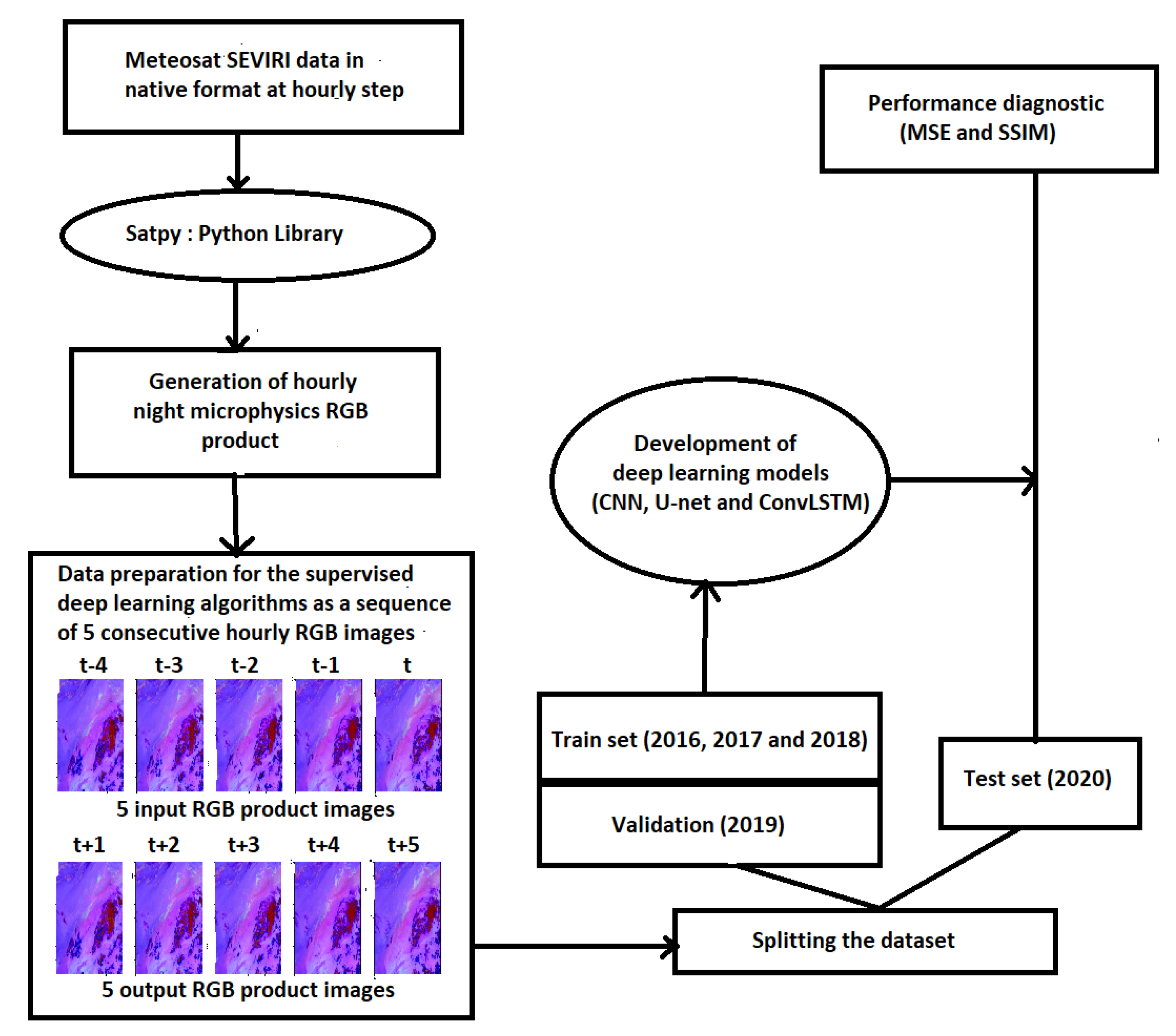
To address this issue, we propose to use several CNN-based architectures [49] that enable the analysis and extraction of the spatial and temporal information in images (Figure 3). A first architecture, that we call CNN, is based on a simple vanilla feedforward multi-layered CNN that takes into account the temporal dimension by concatenating consecutive images over the third axis. The second architecture we consider is based on U-Net [47], which is essentially an encoder–decoder architecture CNN supplemented with skip connections. U-nets are ubiquitous in several image-to-image tasks, especially in segmentation and super resolution. Finally, we use the ConvLSTM architecture [48] based on an image-based extension of the classical LSTM recurrent neural network, and where the data collected are characterized as a time series. In such an approach, the model passes the previous hidden state to the next step of the sequence. Thus, the ConvLSTM determines the future state of a certain cell in the grid by the inputs and past states of its local neighbors. This can easily be achieved by using a convolution operator. The use of such DL approaches for successful weather forecasting applications has been documented in recent years [47,48,49,60,61,62].

2.4.1. Formulation of Fog/Low-Stratus Nowcasting Problem

The goal of fog/low-stratus nowcasting is to use the previously observed satellite images sequence to forecast a fixed length of the future satellite images in a local region. From a machine learning perspective, this problem can be regarded as a spatio-temporal sequence forecasting problem for which an end-to-end DL model is developed, and where both the input and output are spatio-temporal sequences.
Let us suppose that we observe a dynamical system over a spatial region (here, over Morocco) represented by a 661 × 691 grid, which consists of 661 rows (latitudes) and 691 columns (longitudes). Inside each cell in the grid, there are P measurements which vary over time and represent pixel intensity. Thus, the observation at any time can be represented by a tensor X R P × 661 × 691 , where R denotes the domain of the observed features. If we record the observations periodically, we will obtain a sequence of tensors X ^ 1 , X ^ 2 , , X n ^ . Our spatio-temporal sequence forecasting problem is to predict the most likely length-5 sequence in the future given the previous five observations, which include the current one:
X ˜ t + 1 , , X ˜ t + 5 = arg max X t + 1 , , X t + 5 p X t + 1 , , X t + 5 X ^ t 4 , X ^ t 3 , , X ^ t
For fog/low-stratus nowcasting, the observation at every timestamp is a 2D satellite image. If we divide the image into tiled non-overlapping patches and view the pixels inside a patch as its measurements, the nowcasting problem naturally becomes a spatio-temporal sequence forecasting problem. We note that our spatio-temporal sequence forecasting problem is different from the one-step time series forecasting problem because the prediction target of our problem is a sequence which contains both spatial and temporal structures.

2.4.2. Design of Training, Validation and Testing Datasets

To build our ML models, we used 5 years of High Rate SEVIRI Level 1.5 Image Data—MSG—0 degree to create RGB products dataset, from 2016 to 2020 during the cold season (October–April) at an hourly step. For computational convenience, we first normalized the data to the range 0 to 1. Using disjoint subsets for training, testing and validation, we trained our models on RGB product data collected from 2016 to 2018, then they were validated on 2019 data tested on 2020 data.
The data instances are sliced from these blocks using a 5-frame-wide sliding window. Thus our satellite dataset contains 7644 training sequences, 2556 testing sequences and 2544 validation sequences, and all the sequences are 10 frames long (5 for the input X and 5 for the prediction Y). The input data of the model consisted of 5 satellite RGB images (spanning 5 h) and our goal was to forecast the cloud cover for the next 5 h.

2.4.3. Hyperparameter Tuning

The process of setting the hyperparameters requires expertise and extensive trial and error. Deep learning models are full of hyperparameters, and finding the best configuration for these parameters in such a high-dimensional space is not a trivial challenge [63]. In fact, there are some hyperparameters that determines the network structure, such as the kernel size, number of hidden layer, the type of activation functions, and other hyper-parameters that determine the optimal trained network, such as the learning rate and the batch size. While the hyperparameters’ values have a significant impact on the performance of deep neural networks, we performed many configurations and hyperparameter strategies to find the best combination between them. Due to our computing capacity constraints, we will present only the sensitivity of the developed models with regard to the number of filters [64].

2.5. Diagnostic Metrics

2.5.1. Mean Squared Error (MSE)

Once the models were trained with the data, we computed the mean squared error (MSE) of the models for each of the five output time steps. Define M i as the forecast of the model and O i as the corresponding real observational value, with i = 1, ⋯, N, and N as the number of samples.
M S E = 1 N i = 1 N M i O i 2

2.5.2. Structural Similarity Index Measure (SSIM)

In order to remedy some of the issues associated with MSE for image comparison that are explained below, we used the structural similarity index, developed in Ref. [65]:
SSIM ( x , y ) = 2 μ x μ y + c 1 2 σ x y + c 2 μ x 2 + μ y 2 + c 1 σ x 2 + σ y 2 + c 2
with the following:
  • μ x the average of x;
  • μ y the average of y;
  • σ x 2 the variance of x;
  • σ y 2 the variance of y;
  • σ x y the covariance of x and y;
  • c 1 = k 1 L 2 , c 2 = k 2 L 2 two variables to stabilize the division with weak denominator;
  • L the dynamic range of the pixel values (typically, this is 2 bits per pixel 1 ;
  • k 1 = 0.01 and k 2 = 0.03 by default.
In the SSIM formulation, the structural information is decomposed into three components: luminance, contrast and structure. The SSIM attempts to model the perceived change in the structural information of the image, whereas MSE is actually estimating the perceived errors. There is a subtle difference between the two metrics. Indeed, Equation (5) is used to compare two windows (i.e., small sub-samples) rather than the entire image as in MSE. Doing this leads to a more robust approach that is able to account for changes in the structure of the image, rather than just the perceived change. The parameters of Equation (5) include the (x, y) location of the N × N window in each image, the mean of the pixel intensities in the x and y direction, the variance of intensities in the x and y direction, along with the covariance. Unlike MSE, the SSIM value can vary between −1 and 1, where 1 indicates perfect similarity.
It is vital to create a baseline for any time-series prediction approach. As a reference, for comparing all developed models, this baseline can show how well a model makes predictions. The persistence model is one of the most commonly used in the literature for reduced visibility forecasting (e.g., [23]). In the persistence model, it is supposed that the RGB product image expected for the next 5 h is the same as that used as input at time t.

3. Results

Given the different theoretical background between the two categories of techniques adopted in this work, the analysis of the results will be carried out separately for the optical flow (sparse and dense) and the other deep learning techniques (traditional CNN, U-Net and ConvLSTM) on the same case study of 18–19 February 2020. This will allow better conclusions to be drawn on the performance of the used techniques by category. This case study is characterized by a persistent fog event that occurred over the northwestern part of Morocco from 18 UTC on 18 February 2020 (onset phase) to 06 UTC on 19 February 2020 (configuration with mid-/high-level clouds moving over FLS that is not visible anymore). Based on the observed visibilities and clouds at the synoptic stations, the METAR stations show FLS, where FLS is also shown by the RGB product generated from Meteosat SEVIRI satellite data.

3.1. Hyperparameter Tuning

As a preliminary phase, we conducted hyperparameter tuning of the deep learning models in order to determine the best configuration of each developed model. We focused on the number of filters. For the optical flow techniques, the focus is made on the sensitivity of the sparse group to the mask definition on the target phenomenon.

3.1.1. Sensitivity of Optical Flow Techniques to Mask Definition

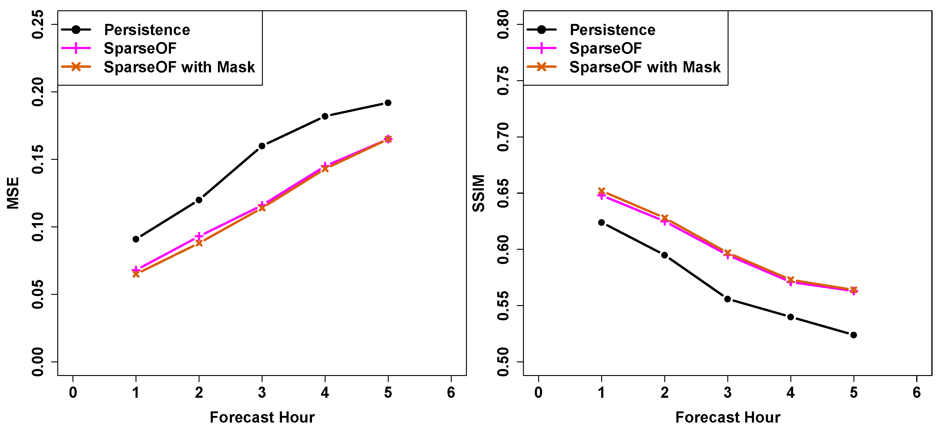
After running many experiments, over other case studies, we found that the sparse optical flow technique performance is highly dependent on the mask definition of the area impacted by the FLS event. To illustrate this, a comparison was performed between the predicted RGB product using this technique with and without mask definition over the area of interest for the case study of 21 November 2020. This event is characterized by the occurrence of FLS layers in the northwestern part of Morocco and another cloud close to this area that appears more intense than the FLS layer (not shown). As a result of the forecasting process, the sparse optical flow model did not capture the position of the fog layer well due to its low intensity. In fact, most of the selected pixels belong to the neighbor cloud area, which is dominant over the study domain (see Figure S1 in Supplementary Materials). Its performance depends also on the features of the input images used to run the model that should contain the FLS layer over the area of interest and must appear clearly with features easily identified by the sparse model using the Shi–Tomasi corner detector. Based on MSE and SSIM (Figure 4) distribution of sparse optical flow with and without mask definition as a function of the forecast hour for this case study, it is seen that sparse optical flow with mask definition slightly outperforms the other configuration and also the persistence, particularly during the two first forecast hours.

3.1.2. Tuning the Number of Filters for Deep Learning Models

Regarding deep learning techniques, one of the downsides of neural networks is their high number of hyperparameters, which requires practitioners to determine the exact model architecture or use automatic hyperparameter-tuning tools, which are time consuming. One important hyperparameter of the CNN is the number of filters. Based on three options for the number of filters (64, 128 and 192), we found that the best configurations for CNN, ConvLSTM and Unet are associated with 64, 128 and 64 filters, respectively. However, we cannot claim that these choices are optimal since the tuning was based on trial and error. To illustrate this, a comparison was performed between the predicted RGB product by DL models (CNN, Unet and ConvLSTM) for the case study of 18–19 February 2020 using the SSIM metric. We plot in Figure 5 the average SSIM over the study domain of each of the three models and the persistence as a function of the forecast hour, for all configurations of filters number (64, 128 and 192). It is seen clearly from this figure that each DL model performs better than the persistence and that the prediction becomes worse for later forecast hours. Based on SSIM, CNN with 64 filters, Unet with 64 filters and ConvLSTM with 128 filters outperform the other configurations slightly.

3.2. Case Study: Optical Flow Techniques Performance

The analysis of the sparse and dense optical flows performance aims to assess the ability of such techniques in tracking and predicting the spatio-temporal evolution of the whole FLS life cycle during the night with mid-/high-level clouds moving over it.
To achieve this, we run four configurations based on one-hour translation and using five RGB product images as input and obtaining five images as nowcasting outputs. Since the sparse and dense optical flow models calculation is based on the intensity to detect the features, we convert first the images to grayscale. The four configurations are summarized in Figure 6.
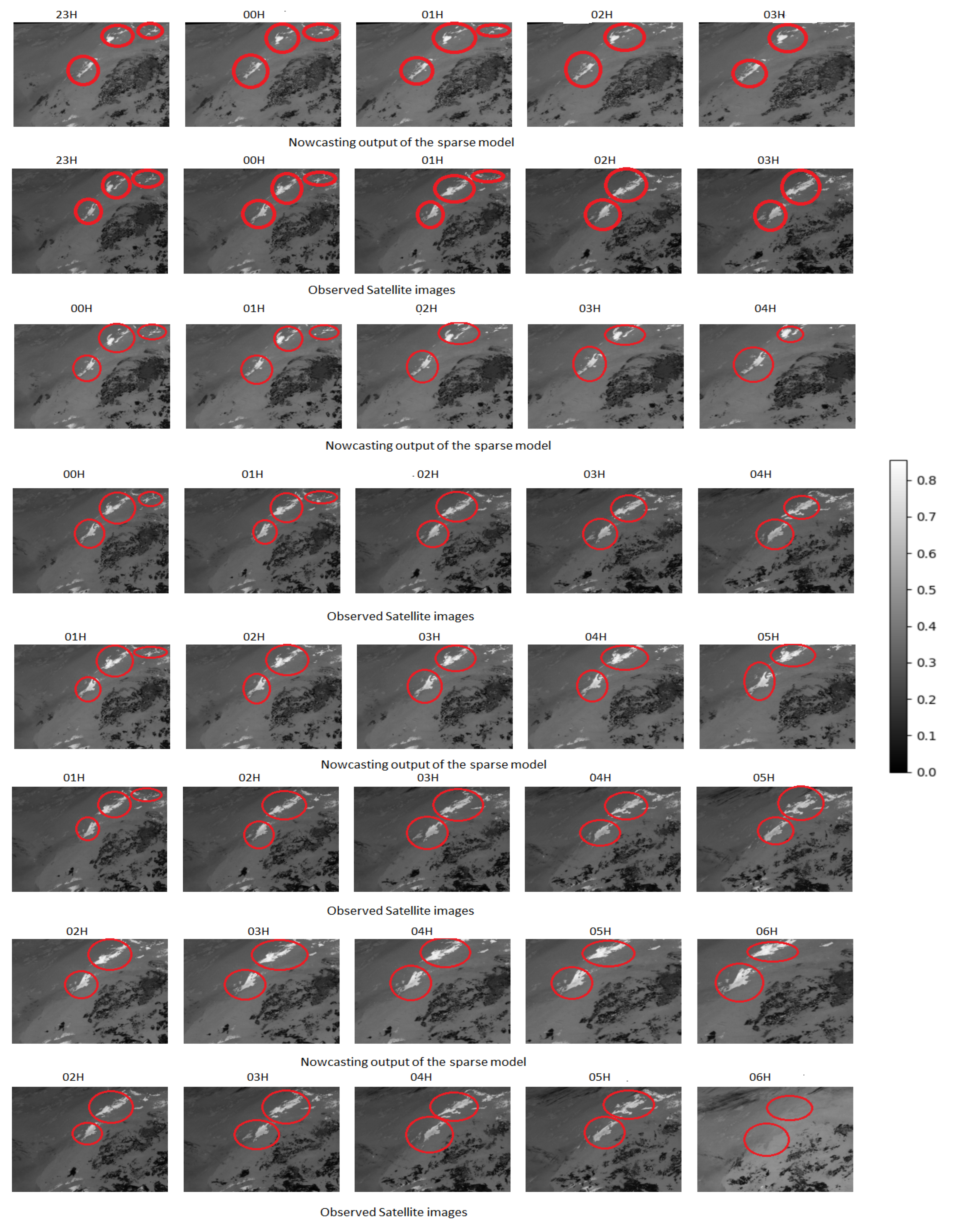
Results analysis from the output of the configuration 1, which represents the transition from the FLS onset to its mature phase, the FLS covers a wide area in the northwestern part of Morocco and the coastal cities on the Mediterranean Ocean side. The input data contain the images from the 18 UTC to 22 UTC of 18 February 2020. Once the features were detected from the input images by the Shi–Tomasi corner detector, the fog area was tracked by the Lucas–Kanade function (row 1 in Figure 7 for SOF and Figure 8 for DOF). Then, a linear regression model was built for every detected feature on images to calculate its new coordinates for every lead time. In comparison with the ground truth (row 2 in Figure 7 for SOF and Figure 8 for DOF), we can see that both optical flow techniques captured well the occurrence of the FLS during the next five hours (since it was present in the input images), but they highly underestimated the spatial coverage of the FLS layer as it develops during its mature phase. Indeed, new corners appeared in relation with the increasing spatial coverage of the fog layer during this phase. These new corners were not taken into account during the corners detection by Shi–Tomasi function and velocity calculation.
Results analysis from the output of configuration 2 and 3 (rows 3 and 5 in Figure 7 for SOF and Figure 8 for DOF) points out that these two configurations show a clear delineation of the spatial coverage of FLS in the mature phase. Thus, the Shi–Tomasi function detects most of the corners related to the area of interest. Therefore, the forecasting process reproduces well the spatio-temporal evolution of the studied fog layer from 00 UTC to 05 UTC on 19 February 2020. The fourth configuration covers from FLS mature phase to its dissimulation by mid-level clouds (row 7 in Figure 7 for SOF and Figure 8 for DOF). As expected, the output of this configuration shows clearly that both techniques miss this coverage by the mid-level cloud and predict a well-developed FLS layer since the principle of the optical flow is tracking and extrapolation.
From each studied configuration, the sparse and dense optical-flow-based models used to forecast future satellite images showed significant skill for the two first lead times. Yet, from the third forecast hour, a decrease in model skill is observed for most of the configurations. This loss of information could be attributed to the errors introduced in corner tracking since this model is based on identifying distinct features in the satellite images. From the last configuration, we found that it is pretty difficult for sparse and dense optical flow models to well predict a sudden dissimulation of the fog by a large mid-level cloud and not even the development of new areas of FLS.

3.3. Case Study: Deep Learning Techniques Performance

This section is dedicated to the quantitative and qualitative assessments of the deep learning techniques (CNN, U-net and ConvLSTM) performance in nowcasting the whole life cycle of the same FLS event used for the assessment of the optical flow techniques. To achieve this, we run four configurations based on one-hour translation, as for the optical flow techniques, with 5 RGB images as input and obtaining 5 RGB images as output.
To assess quantitatively the performance of the ML-developed models (CNN, Unet and ConvLSTM) for this case study, we plotted on Figure 9 the distribution of the average MSE and SSIM over the study domain of each of the three DL models, the two optical flow models and the persistence as function of the forecast hour. For the interpretation of the SSIM score, the maximum value of 1 indicates that the two signals are perfectly structurally similar while a value of 0 indicates no structural similarity. On the other hand, the best performance of a machine learning based model using MSE is associated with the one that has the minimum value of this error and which tends to zero.
It is seen clearly from Figure 9 that each DL model performs better than the persistence and the optical flow algorithms, and that the prediction becomes worse for later forecast hours. Figure 9 reveals that the MSE of all techniques increases as a function of the lead time. This indicates the best performance for the two forecast hours and points out the usefulness of the DL techniques for RGB product images nowcasting. It is als found from these figures that CNN outperforms clearly the persistence and the other DL techniques for this use case.
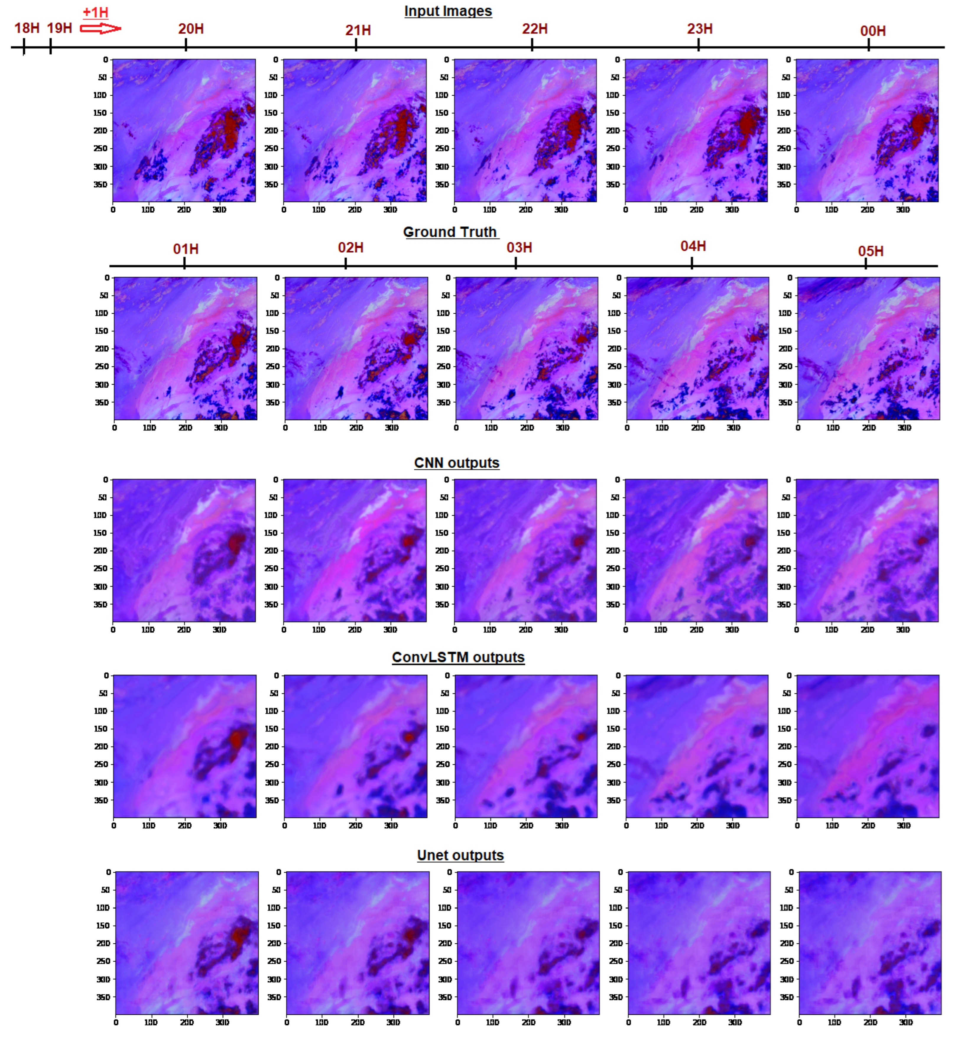
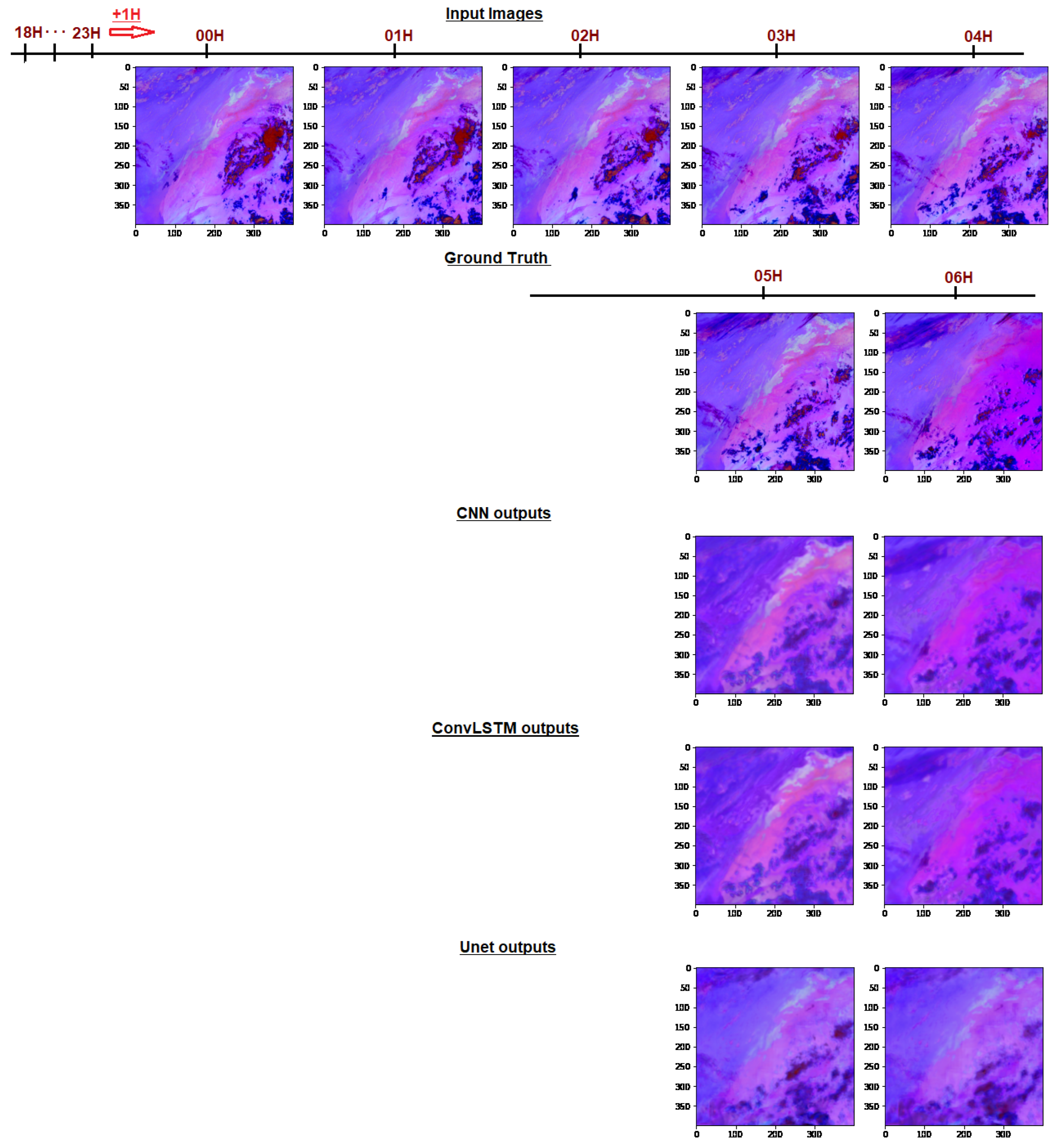
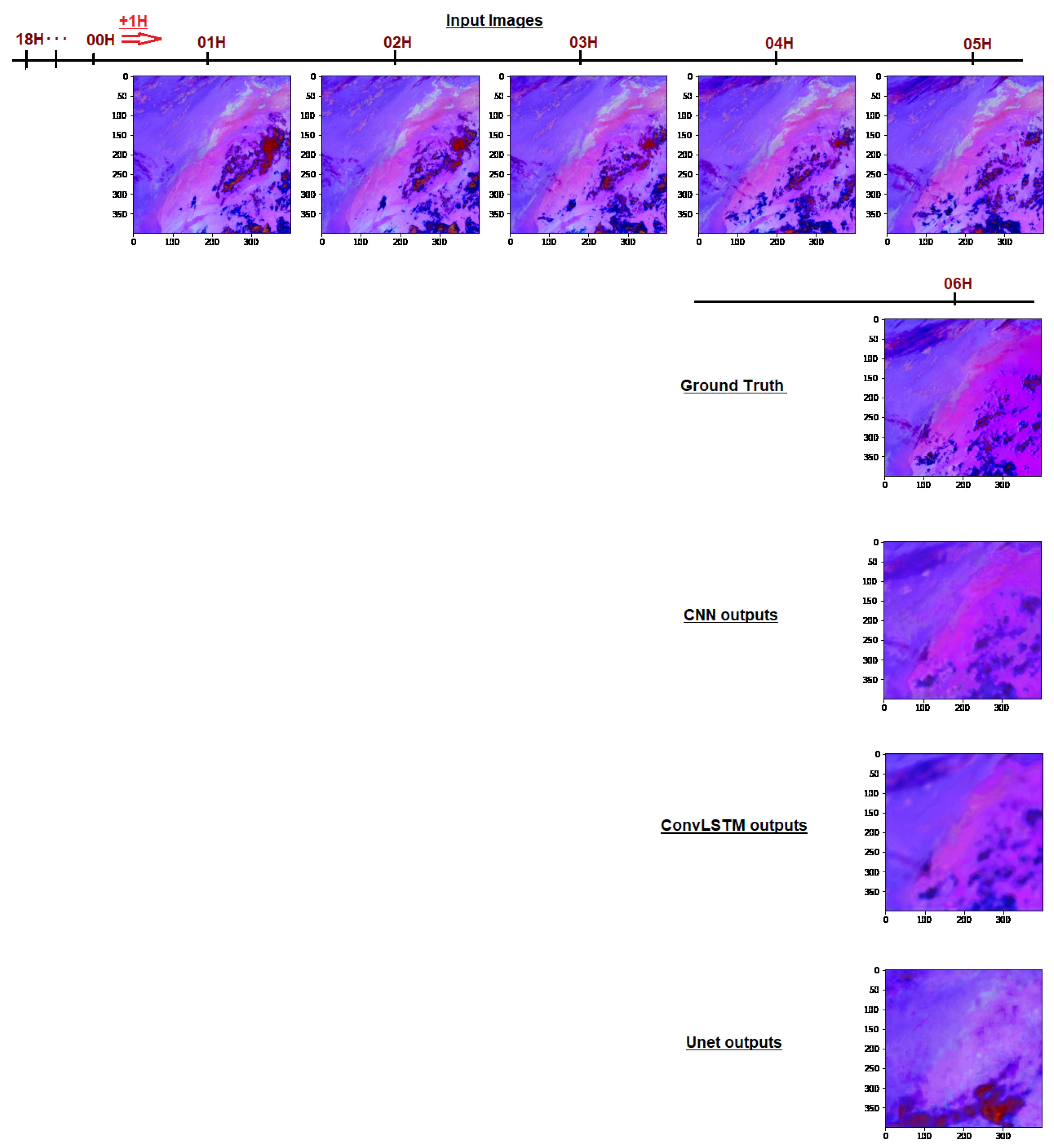
To assess qualitatively the performance of the ML-developed models (CNN, Unet and ConvLSTM) for this case study, Figure 10 and Figure 11 show the transition from the FLS onset to its mature phase, while Figure 12 and Figure 13 represent the phase when the mid-/high-level cloud moves over FLS and the FLS is not visible anymore. In addition, the first row in these figures represents the input hourly images for the three DL models (CNN, Unet and ConvLSTM). The ground truth (observation) and predicted images (from CNN, ConvLSTM and Unet) representing the meteorological situation for the next 5 h, are plotted respectively in rows 2 to 5 on the same figures. It should be noted that the night microphysics RGB product is useful only during the night from 1800 UTC day (d) until 0600 UTC day (d + 1).
It is seen clearly from these figures, supported by Figure 9, that the closer the input images are to the predicted time, the higher the quality of the forecast for the different DL models. The CNN model proved to be the most accurate in tracking and nowcasting the development of fog and low clouds, as well as anticipating their dissimulation by mid-level clouds (Figure 9). On the other hand, while not as well trained as the other two models, due to the large number of parameters it has to adjust, the ConvLSTM model succeeds in predicting the location and shape of fog and low clouds, with the exception that their intensity is less than in reality, which can be corrected with extra training. For the Unet model, it manages to follow the development of the studied FLS events better than ConvLSTM.
By comparing the models based on their SSIM values, ConvLSTM produced a comparable outcome to CNN and Unet overall lead times. This could be explained by the temporal component that is integrated in ConvLSTM architecture. In fact, the ConvLSTM has a large number of parameters, which makes its training difficult using our available computing capacity (Google Colab has been used in this study as a free GPU runtime environment). Despite the fact that we could not train the ConvLSTM until complete convergence, its performance is still acceptable, and it is expected that ConvLSTM might outperform the other models with better computing resources than those used in this work.
Based on the qualitative and quantitative assessment of the developed models on this case study, one can conclude that CNN and Unet models were successful in predicting the evolution of the studied FLS position and coverage, particularly during the first three forecast hours. This proves that some of the complex spatio-temporal patterns in the dataset can be learned by the nonlinear and convolutional structure of the network.

3.4. Global Performance Assessment over the Test Data Set

Table 1 summarizes the quantitative assessment of both optical flow and deep learning techniques in terms of MSE and SSIM over the test dataset (cold season of 2020). It is seen clearly that ConvLSTM achieves the best performance on both metrics. To be specific, ConvLSTM achieves a performance gain by 3.2% (6.2%), 7.5% (11.8%), 22.2% (22.9%), 29.4% (26.2%) and 49% (36%) on SSIM (respectively, MSE) in comparison with Unet, CNN, DOF, SOF and persistence, respectively.
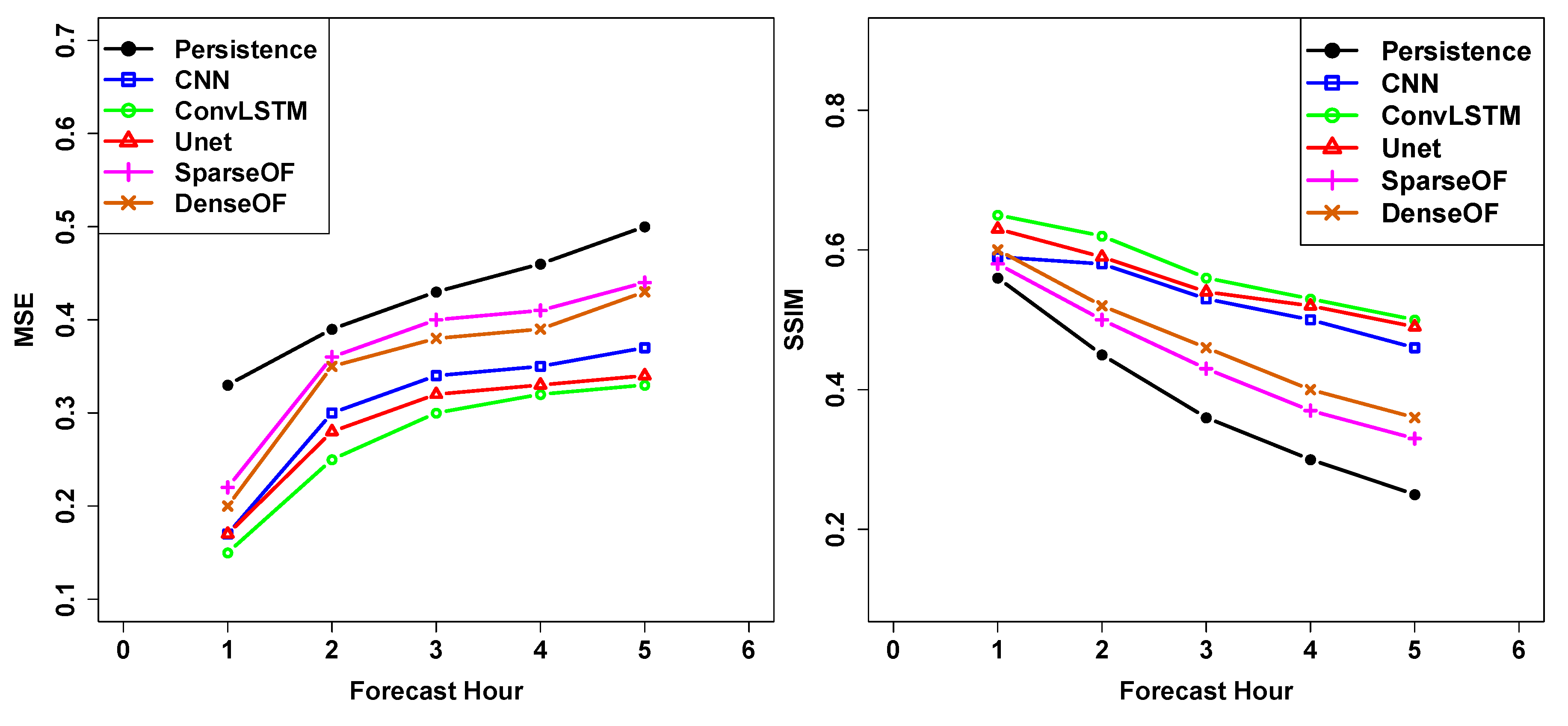
Figure 14 represents the MSE and SSIM metrics distribution as function of forecast hour for CNN, ConvLSTM, Unet, SparseOF and DenseOF over the test data set. Persistence scores are also drawn as benchmarks. A common result between the different DL models is that the closer the input images are to predicted time, the higher the quality of the forecast. As the forecast time progresses, the quality of the prediction decreases, particularly from the third time step. This demonstrates the usefulness of these techniques in the nowcasting purpose.

4. Discussion

In this study, the used DL models provide a predicted night microphysics RGB product image, and it is up to the forecaster to identify the areas of interest for the FLS events based on their apparent color. The climatology of FLS over the study domain in the year 2020 is found to be similar to that over the training period 2016–2019. Indeed, most of the observed FLS over the synoptic stations occurred in the evening and at the end of night. The FLS events often last no longer than 3 h. Consequently, deep learning techniques are expected to learn this global aspect from the training sample and reflect it in the forecast process. This was verified in a subjective way, where some cases were checked visually. In such cases, the FLS was observed in the northwestern part of Morocco (the FLS prone region as demonstrated by Bari et al. [8]). However, due to the lack of labeled data, it was pretty difficult to assess quantitatively the performance of the DL models regarding the FLS prediction. Indeed, while the used supervised deep learning techniques require a great amount of labeled data to train a model in the classification framework [66], the availability of labeled training data is extremely limited owing to the nature of the FLS phenomenon (e.g., spatial coverage, occurrence time and duration).
Based on a visual comparison of the output RGB product related to FLS occurrence only with the truth images, we found that all DL models successfully predicted in many cases the FLS area with large coverage over the northwestern part of Morocco that already exist in the input images, while it is still challenging for these techniques to predict the emergence of new FLS areas. This is in line with the findings of [67], which indicated that these same models and all other extrapolation techniques are incapable of forecasting the emergence of new clouds. This could be due to the lack of sufficient training data that cover such configuration. The scarcity of labeled satellite images with ground truth information about the exact timing and location of cloud formation hampers the model’s ability to learn the complex dynamics associated with cloud emergence. While deep learning models can learn intricate patterns from data, their predictive capability can be limited if they lack explicit knowledge about these underlying processes. Another possible explanation for this limitation is the fact that when applied to satellite image forecasting, models may become too specific to the training dataset, failing to generalize well to new or unseen cloud patterns. The lack of diversity and representativeness in the training data can contribute to this issue. It should be noted that while ConvLSTM predicted well the location and the shape of the FLS areas in many use cases, it did not correctly assign the FLS color (RGB value), where their intensity is less than in reality. This could be explained by the mean square error metric, which tends to smooth the results because of the L2 norm.In fact, ConvLSTMs are designed to model sequential data and retain long-term dependencies. However, if the temporal dynamics involved in FLS formation are highly complex or exhibit nonlinear patterns, even ConvLSTMs may struggle to capture the precise timing and location of FLS emergence. One way to improve the performance of deep learning techniques for predicting the emergence of new clouds is exploring approaches such as incorporating physical models, integrating additional meteorological data, using more sophisticated network architectures, using transfer learning (VGG [68] and ResNet [69]), and collecting larger and more diverse datasets that accurately represent the range of cloud formation processes.
In the big data era, the download and storage costs are two aspects that make data availability difficult due to the fact that Earth observation images are complex and very large [70]. The data preparation step before DL models development (creation of RGB product, generation of sequences that contain five consecutive hourly images, etc.) requires a significant amount of time and the intervention of an expert in the remote sensing field who knows the specific information to extract depending on the problem that needs solving. To overcome this shortcoming, some workflows and libraries are emerging as open-source tools to facilitate the data preparation step of satellite images (Satpy Python library [56] was used in this work to generate RGB products from native files).
Regarding the application of optical flow techniques for FLS nowcasting, it is found that the sparse group is very sensitive to the feature detection in the input images. In fact, establishing an automatic and dynamic function to define a mask over the area interested by the target phenomenon is still a challenge. Some recent research studies [71] tried to deal with this issue. The authors of [71] developed a new method that integrates mask region-based convolutional neural network and k-means with the Lucas–Kanade algorithm. One other possible solution consists of keeping only the areas covered by the target phenomenon and trying to follow its movement. Incorporating additional contextual information, such as meteorological parameters, topographical data, or atmospheric models, into the optical flow calculations can also provide valuable insights and constraints that enhance the accuracy and relevance of the optical flow estimation.
The dense group managed well to predict a significant area covered by FLS over the study domain, particularly during the two first hours. However, the forecasting performance decreases for the later forecast hours. Overall, while optical flow techniques can provide valuable insights into the movement of FLS patterns based on satellite imagery, they are subject to several limitations that can impact their accuracy and reliability for forecasting purposes. One strategy to overcome these limitations consists of ensuring that the satellite imagery data used for optical flow calculations is of high quality. In addition, optical flow techniques rely on the assumption of temporal consistency between consecutive frames. However, the hourly time interval between frames adopted in this work can be large, resulting in significant changes in cloud patterns or other meteorological phenomena. To address this, consider that reducing the temporal windows (15 min) could help the model capture the evolving dynamics more effectively. The combination of optical flow and deep learning can leverage the strengths of both techniques and mitigate their individual limitations (FlowNet [72,73] and DeepFlow [74]).

5. Conclusions

In this paper, we applied for the first time optical flow (sparse and dense) and deep learning techniques (CNN, ConvLSTM and Unet) to geostationary satellite images for fog/low-stratus (FLS) nowcasting through the night microphysics RGB product. This work is innovative since the RGB product prediction is regarded as a spatiotemporal sequence-forecasting problem, for which an end-to-end optical flow and deep learning model were developed, and where both the input and output are spatiotemporal sequences. To achieve this goal, two datasets of hourly observation (visibility and low cloudiness) from METARs of 43 synoptic stations and Meteosat SEVIRI image data (in native format to generate night microphysics RGB product), covering the cold and FLS prone season (October to April) over a 5-year period (2016–2020), were used. The performance of the developed models was evaluated through many case studies visually and quantitatively using MSE and SSIM metrics. The following three main conclusions could be drawn from this research work:
1.
ConvLSTM outperforms conventional CNN and Unet algorithms and state-of-the art of optical flow techniques (sparse and dense) over all lead times. This method is superior in terms of both MSE and SSIM metrics with values of about 0.3 and 0.6, respectively.
2.
The DL algorithms can better model the nonlinear processes of the evolution of FLS event and produce more reasonable and location-accurate nowcasts. A representative case study qualitatively illustrates that DL models can better model the spatiotemporal evolution of FLS event and its coverage by mid-level clouds and produce more reasonable nowcasts, while the optical flow techniques fails in reproducing this configuration.
3.
The sparse optical flow technique showed high sensitivity to the mask definition on the area of interest and also the target phenomenon, while for deep learning techniques, it was found that the number of filters tuning has an impact on the performance of the DL-based models.
Although the quantitative and qualitative comparison and analysis verify the superiority and effectiveness of DL techniques for extrapolation-based RGB product nowcasting, some limitations remain, and our study can be extended in several directions. First, to cover the FLS nowcasting during the whole day, it would be interesting to use different RGB composites, such as SEVIRI HRV Fog RGB or 24 h microphysics RGB. Second, the conventional approach of designing and training new convolutional neural networks (CNNs) from scratch for various tasks can be time consuming in order to achieve optimal configurations. With increasingly powerful computational resources, another interesting way of improvement is to take advantage of transfer learning to train satellite data on pretrained models, such as the VGG [68] and ResNet [69] series networks and adjusting them to learn a new task. Additionally, the recent developments in transformer-based architectures can be a promising follow-up to this work.

Supplementary Materials

The following supporting information can be downloaded at: https://www.mdpi.com/article/10.3390/atmos14060953/s1, Figure S1. The output of the Shi–Tomasi corner detector: (left) without and (right) with predefined mask over the area of interest. Case study of 21 November 2020, which is characterized by the occurrence of FLS layers in the north-western part of Morocco and very thick, more intense clouds close to this area. The red points refer to the most prominent corners in the image based on the calculation of the corner quality measure at each pixel.

Author Contributions

Conceptualization, D.B. and R.L.; methodology, D.B.; software, N.L.; validation, D.B. and R.L.; formal analysis, N.L. and R.S.; investigation, all the authors; data curation, N.L. and R.S.; writing—original draft preparation, D.B.; writing—review and editing, D.B. and R.L. All authors have read and agreed to the published version of the manuscript.

Funding

This research received no external funding.

Institutional Review Board Statement

Not applicable.

Informed Consent Statement

Not applicable.

Data Availability Statement

The observation data from the Moroccan synoptic network that support the findings of this study are available on request from the Moroccan General Directorate (DGM, https://www.marocmeteo.ma, accessed on 10 February 2021). The data are not publicly available due to commercialization restrictions. The High Rate SEVIRI Level 1.5 Image Data-MSG-0 degree can be freely extracted from the Earth Observation Portal of EUMETSAT ( https://eoportal.eumetsat.int/, accessed on 10 February 2021) in different format.

Acknowledgments

We would like to thank the three anonymous reviewers for taking the time and effort necessary to review the manuscript. We sincerely appreciate all valuable comments and suggestions, which helped us to improve the quality of the manuscript.

Conflicts of Interest

The authors declare no conflict of interest.

References

  1. Leigh, R.J.; Drake, L.; Thampapillai, D.J. An Economic Analysis of Terminal Aerodrome Forecasts with Special Reference to Sydney Airport. J. Transp. Econ. Policy 1998, 55, 1731–1745. [Google Scholar]
  2. Pagowski, M.; Gultepe, I.; King, P. Analysis and Modeling of an Extremely Dense Fog Event in Southern Ontario. J. Appl. Meteorol. 2004, 43, 3–16. [Google Scholar] [CrossRef]
  3. Kneringer, P.; Dietz, S.J.; Mayr, G.J.; Zeileis, A. Probabilistic nowcasting of low-visibility procedure states at Vienna International Airport during cold season. Pure Appl. Geophys. 2019, 176, 2165–2177. [Google Scholar] [CrossRef]
  4. Dietz, S.J.; Kneringer, P.; Mayr, G.J.; Zeileis, A. Low-visibility forecasts for different flight planning horizons using tree-based boosting models. Adv. Stat. Climatol. Meteorol. Oceanogr. 2019, 5, 101–114. [Google Scholar] [CrossRef]
  5. Haeffelin, M.; Bergot, T.; Elias, T.; Tardif, R.; Carrer, D.; Chazette, P.; Colomb, M.; Drobinski, P.; Dupont, E.; Dupont, J.-C.; et al. Parisfog. Bull. Am. Meteorol. Soc. 2010, 91, 767–783. [Google Scholar] [CrossRef]
  6. Wang, Y.; Niu, S.; Lu, C.; Lv, J.; Zhang, J.; Zhang, H.; Shao, N.; Sun, W.; Jin, Y.; Song, Q. Observational study of the physical and chemical characteristics of the winter radiation fog in the tropical rainforest in Xishuangbanna, China. Sci. China Earth Sci. 2021, 64, 1982–1995. [Google Scholar] [CrossRef]
  7. Wang, Y.; Lu, C.; Niu, S.; Lv, J.; Jia, X.; Xu, X.; Xue, Y.; Zhu, L.; Yan, S. Diverse dispersion effects and parameterization of relative dispersion in urban fog in eastern China. J. Geophys. Res. Atmos. 2023, 128, e2022JD037514. [Google Scholar] [CrossRef]
  8. Bari, D.; Bergot, T.; El Khlifi, M. Local meteorological and large-scale weather characteristics of fog over the grand Casablanca region, morocco. J. Appl. Meteorol. Climatol. 2016, 55, 1731–1745. [Google Scholar] [CrossRef]
  9. Kim, W.; Yum, S.S.; Hong, J.; Song, J.I. Improvement of Fog Simulation by the Nudging of Meteorological Tower Data in the WRF and PAFOG Coupled Model. Atmosphere 2020, 11, 311. [Google Scholar] [CrossRef]
  10. Liu, Q.; Wu, B.; Wang, Z.; Hao, T. Fog Droplet Size Distribution and the Interaction between Fog Droplets and Fine Particles during Dense Fog in Tianjin, China. Atmosphere 2020, 11, 258. [Google Scholar] [CrossRef]
  11. Leung, A.C.W.; Gough, W.A.; Butler, K.A. Changes in Fog, Ice Fog, and Low Visibility in the Hudson Bay Region: Impacts on Aviation. Atmosphere 2020, 11, 186. [Google Scholar] [CrossRef]
  12. Bari, D.; Bergot, T.; El Khlifi, M. Numerical study of a coastal fog event over casablanca, morocco. Q. J. R. Meteorol. Soc. 2015, 141, 1894–1905. [Google Scholar] [CrossRef]
  13. Boutle, I.; Angevine, W.; Bao, J.-W.; Bergot, T.; Bhattacharya, R.; Bott, A.; Ducongé, L.; Forbes, R.; Goecke, T.; Grell, E.; et al. Demistify: A large-eddy simulation (LES) and single-column model (SCM) intercomparison of radiation fog. Atmos. Chem. Phys. 2022, 22, 319–333. [Google Scholar] [CrossRef]
  14. Bergot, T.; Koracin, D. Observation, simulation and predictability of fog: Review and perspectives. Atmosphere 2021, 12, 235. [Google Scholar] [CrossRef]
  15. Cermak, J.; Bendix, J. Dynamical nighttime fog/low stratus detection based on Meteosat SEVIRI data: A feasibility study. Pure Appl. Geophys. 2007, 164, 1179–1192. [Google Scholar] [CrossRef]
  16. Gautam, R.; Singh, M.K. Urban Heat Island Over Delhi Punches Holes in Widespread Fog in the Indo-Gangetic Plains. Geophys. Res. Lett. 2018, 45, 1114–1121. [Google Scholar] [CrossRef]
  17. Fuchs, J.; Andersen, H.; Cermak, J.; Pauli, E.; Roebeling, R. High-resolution satellite-based cloud detection for the analysis of land surface effects on boundary layer clouds. Atmos. Meas. Tech. 2022, 15, 4257–4270. [Google Scholar] [CrossRef]
  18. Egli, S.; Thies, B.; Drönner, J.; Cermak, J.; Bendix, J.; Thies, B.; Bendix, J. A 10 year fog and low stratus climatology for Europe based on Meteosat Second Generation data. Q. J. R. Meteorol. Soc. 2017, 143, 530–541. [Google Scholar] [CrossRef]
  19. Bari, D.; El Khlifi, M. LVP conditions at Mohamed v airport, Morocco: Local characteristics and prediction using neural networks. Int. J. Basic Appl. Sci. 2015, 4, 354. [Google Scholar] [CrossRef]
  20. Dueben, P.; Bauer, P. Challenges and design choices for global weather and climate models based on machine learning. Geosci. Model Dev. 2018, 11, 3999–4009. [Google Scholar] [CrossRef]
  21. Chkeir, S.; Anesiadou, A.; Mascitelli, A.; Biondi, R. Nowcasting extreme rain and extreme wind speed with machine learning techniques applied to different input datasets. Atmos. Res. 2023, 282, 106548. [Google Scholar] [CrossRef]
  22. Bari, D. Visibility prediction based on kilometric nwp model outputs using machine-learning regression. In Proceedings of the 2018 IEEE 14th International Conference on e-Science (e-Science), Amsterdam, The Netherlands, 29 October–1 November 2018; p. 278. [Google Scholar]
  23. Bari, D.; Ouagabi, A. Machine-learning regression applied to diagnose horizontal visibility from mesoscale nwp model forecasts. SN Appl. Sci. 2020, 2, 1–13. [Google Scholar] [CrossRef]
  24. Ravuri, S.; Lenc, K.; Willson, M.; Kangin, D.; Lam, R.; Mirowski, P.; Fitzsimons, M.; Athanassiadou, M.; Kashem, S.; Madge, S.; et al. Skilful precipitation nowcasting using deep generative models of radar. Nature 2021, 597, 672–677. [Google Scholar] [CrossRef] [PubMed]
  25. Lam, R.; Sanchez-Gonzalez, A.; Willson, M.; Wirnsberger, P.; Fortunato, M.; Pritzel, A.; Ravuri, S.; Ewalds, T.; Alet, F.; Eaton-Rosen, Z.; et al. GraphCast: Learning skillful medium-range global weather forecasting. arXiv 2022, arXiv:2212.12794. [Google Scholar]
  26. Pritt, M.; Chern, G. Satellite image classification with deep learning. In Proceedings of the 2017 IEEE Applied Imagery Pattern Recognition Workshop (AIPR), Washington, DC, USA, 10–12 October 2017; pp. 1–7. [Google Scholar]
  27. Alkhelaiwi, M.; Boulila, W.; Ahmad, J.; Koubaa, A.; Driss, M. An efficient approach based on privacy-preserving deep learning for satellite image classification. Remote Sens. 2021, 13, 2221. [Google Scholar] [CrossRef]
  28. Zhang, P.; Ke, Y.; Zhang, Z.; Wang, M.; Li, P.; Zhang, S. Urban land use and land cover classification using novel deep learning models based on high spatial resolution satellite imagery. Sensors 2018, 18, 3717. [Google Scholar] [CrossRef] [PubMed]
  29. Pan, Z.; Xu, J.; Guo, Y.; Hu, Y.; Wang, G. Deep learning segmentation and classification for urban village using a worldview satellite image based on U-Net. Remote Sens. 2020, 12, 1574. [Google Scholar] [CrossRef]
  30. Li, L.; He, Z.; Chen, S.; Mai, X.; Zhang, A.; Hu, B.; Li, Z.; Tong, X. Subpixel-Based Precipitation Nowcasting with the Pyramid Lucas–Kanade Optical Flow Technique. Atmosphere 2018, 9, 260. [Google Scholar] [CrossRef]
  31. Le Goff, M.; Tourneret, J.Y.; Wendt, H.; Ortner, M.; Spigai, M. Deep learning for cloud detection. In Proceedings of the 8th International Conference of Pattern Recognition Systems ICPRS, Madrid, Spain, 11–13 July 2017; pp. 1–6. [Google Scholar]
  32. Zhang, J.; Lu, H.; Xia, Y.; Han, T.; Miao, K.; Yao, Y.; Liu, C.; Zhou, J.P.; Chen, P.; Wang, B. Deep convolutional neural network for fog detection. In Intelligent Computing Theories and Application, Proceedings of the 14th International Conference on Intelligent Computing, Wuhan, China, 15–18 August 2018; Springer: Berlin/Heidelberg, Germany, 2018; pp. 1–10. [Google Scholar]
  33. Guo, S.; Sun, N.; Pei, Y.; Li, Q. 3D-UNet-LSTM: A Deep Learning-Based Radar Echo Extrapolation Model for Convective Nowcasting. Remote Sens. 2023, 15, 1529. [Google Scholar] [CrossRef]
  34. Shi, X.; Chen, Z.; Wang, H.; Yeung, D.Y.; Wong, W.K.; Woo, W.C. Convolutional LSTM network: A machine learning approach for precipitation nowcasting. Adv. Neural Inf. Process. Syst. 2015, 28, 1–9. [Google Scholar]
  35. Petrou, Z.I.; Tian, Y. Prediction of sea ice motion with convolutional long short-term memory networks. IEEE Trans. Geosci. Remote. Sens. 2019, 57, 6865–6876. [Google Scholar] [CrossRef]
  36. Tan, C.; Feng, X.; Long, J.; Geng, L. Forecast-CLSTM: A new convolutional lstm network for cloudage nowcasting. In Proceedings of the 2018 IEEE Visual Communications and Image Processing (VCIP), Taichung, Taiwan, 9–12 December 2018; pp. 1–4. [Google Scholar]
  37. Guo, Y.; Cao, X.; Liu, B.; Gao, M. Cloud detection for satellite imagery using attention-based u-net convolutional neural network. Symmetry 2018, 12, 1056. [Google Scholar] [CrossRef]
  38. Leese, J.A.; Novak, C.S.; Taylor, V.R. The determination of cloud pattern motions from geosynchronous satellite image data. Pattern Recognit. 1970, 2, 279–292. [Google Scholar] [CrossRef]
  39. Ayzel, G.; Heistermann, M.; Winterrath, T. Optical flow models as an open benchmark for radar-based precipitation nowcasting (rainymotion v0. 1), Geosci. Model Dev. 2019, 12, 1387–1402. [Google Scholar] [CrossRef]
  40. Marrocu, M.; Massidda, L. Performance Comparison between Deep Learning and Optical Flow-Based Techniques for Nowcast Precipitation from Radar Images. Forecasting 2020, 2, 194–210. [Google Scholar] [CrossRef]
  41. Wood-Bradley, P.; Zapata, J.; Pye, J. Cloud tracking with optical flow for short-term solar forecasting. In Proceedings of the 50th Conference of the Australian Solar Energy Society, Melbourne, Australia, 10–11 October 2012. [Google Scholar]
  42. Mondragón, R.; Alonso-Montesinos, J.; Riveros-Rosas, D.; Bonifaz, R. Determination of cloud motion applying the Lucas-Kanade method to sky cam imagery. Remote Sens. 2020, 12, 2643. [Google Scholar] [CrossRef]
  43. Zaher, A.Y.; Ghanem, A. Clouds motion estimation from ground-based sky camera and satellite images. In Colorimetry and Image Processing; IntechOpen: London, UK, 2017. [Google Scholar]
  44. Nguyen, T.X.B.; Rosser, K.; Chahl, J. A Comparison of Dense and Sparse Optical Flow Techniques for Low-Resolution Aerial Thermal Imagery. J. Imaging 2022, 8, 116. [Google Scholar] [CrossRef]
  45. Wu, H.; Zhao, R.; Gan, X.; Ma, X. Measuring surface velocity of water flow by dense optical flow method. Water 2019, 11, 2320. [Google Scholar] [CrossRef]
  46. Bari, D.; Bergot, T. Influence of Environmental Conditions on Forecasting of an Advection-Radiation Fog: A Case Study from the Casablanca Region, Morocco. Aerosol Air Qual. Res. 2018, 18, 62–78. [Google Scholar] [CrossRef]
  47. Gu, J.; Wang, Z.; Kuen, J.; Ma, L.; Shahroudy, A.; Shuai, B.; Liu, T.; Wang, W.; Wang, G.; Cai, J.; et al. Recent advances in convolutional neural networks. Pattern Recognit. 2018, 77, 354–377. [Google Scholar] [CrossRef]
  48. Yu, Y.; Si, X.; Hu, C.; Zhang, J. A review of recurrent neural networks: LSTM cells and network architectures. Neural Comput. 2019, 31, 1235–1270. [Google Scholar] [CrossRef] [PubMed]
  49. Ajit, A.; Acharya, K.; Samanta, A. A review of convolutional neural networks. In Proceedings of the 2020 International Conference on Emerging Trends in Information Technology and Engineering (IC-ETITE), Vellore, India, 24–25 February 2020; pp. 1–5. [Google Scholar]
  50. Knippertz, P.; Christoph, M.; Speth, P. Long-term precipitation variability in Morocco and the link to the large-scale circulation in recent and future climates. Meteorol. Atmos. Phys. 2003, 83, 67–88. [Google Scholar] [CrossRef]
  51. Driouech, F.; Déqué, M.; Mokssit, A. Numerical simulation of the probability distribution function of precipitation over Morocco. Clim. Dyn. 2009, 32, 1055–1063. [Google Scholar] [CrossRef]
  52. Tramblay, Y.; El Adlouni, S.; Servat, E. Trends and variability in extreme precipitation indices over North Africa. Nat. Hazards Earth Syst. Sci. 2013, 13, 3235–3248. [Google Scholar] [CrossRef]
  53. Schilling, J.; Hertig, E.; Tramblay, Y.; Scheffran, J. Climate change vulnerability, water resources and social implications in North Africa. Reg. Environ. Chang. 2020, 20, 15. [Google Scholar] [CrossRef]
  54. Eguchi, N.; Hayasaka, T.; Sawada, M. Maritime-continental contrasts in the properties of low-level clouds: A case study of the summer of the 2003 Yamase, Japan, cloud event. Adv. Meteorol. 2014, 2014, 1–16. [Google Scholar] [CrossRef]
  55. Cropper, T.E.; Hanna, E.; Bigg, G.R. Spatial and temporal seasonal trends in coastal upwelling off Northwest Africa, 1981–2012. Deep. Sea Res. Part Oceanogr. Res. Pap. 2014, 86, 94–111. [Google Scholar] [CrossRef]
  56. Hoese, D. SatPy: A Python Library for Weather Satellite Processing. In Proceedings of the 99th American Meteorological Society Annual Meeting, AMS, Madison, WI, USA, 8 January 2019. [Google Scholar]
  57. Fleet, D.; Weiss, Y. Optical flow estimation. In Handbook of Mathematical Models in Computer Vision; Springer: Berlin/Heidelberg, Germany, 2006; pp. 237–257. [Google Scholar]
  58. Zhai, M.; Xiang, X.; Lv, N.; Kong, X. Optical flow and scene flow estimation: A survey. Pattern Recognit. 2021, 114, 107861. [Google Scholar] [CrossRef]
  59. Kaplan, G.; Comert, R.; Kaplan, O.; Matci, D.K.; Avdan, U. Using Machine Learning to Extract Building Inventory Information Based on LiDAR Data. ISPRS Int. J. Geo-Inf. 2022, 11, 517. [Google Scholar] [CrossRef]
  60. Moskolaï, W.R.; Abdou, W.; Dipanda, A. Application of deep learning architectures for satellite image time series prediction: A review. Remote Sens. 2021, 13, 4822. [Google Scholar] [CrossRef]
  61. Valdivia-Bautista, S.M.; Domínguez-Navarro, J.A.; Pérez-Cisneros, M.; Vega-Gómez, C.J.; Castillo-Téllez, B. Artificial Intelligence in Wind Speed Forecasting: A Review. Energies 2023, 16, 2457. [Google Scholar] [CrossRef]
  62. Naranjo-Torres, J.; Mora, M.; Hernández-García, R.; Barrientos, R.J.; Fredes, C.; Valenzuela, A. A review of convolutional neural network applied to fruit image processing. Appl. Sci. 2020, 10, 3443. [Google Scholar] [CrossRef]
  63. Yang, L.; Shami, A. On hyperparameter optimization of machine learning algorithms: Theory and practice. Neurocomputing 2020, 415, 295–316. [Google Scholar] [CrossRef]
  64. Xiao, X.; Yan, M.; Basodi, S.; Ji, C.; Pan, Y. Efficient hyperparameter optimization in deep learning using a variable length genetic algorithm. arXiv 2020, arXiv:2006.12703. [Google Scholar]
  65. Wang, Z.; Bovik, A.C.; Sheikh, H.R.; Simoncelli, E.P. Image quality assessment: From error visibility to structural similarity. IEEE Trans. Image Process. 2004, 13, 600–612. [Google Scholar] [CrossRef]
  66. Li, Y.; Zhang, H.; Xue, X.; Jiang, Y.; Shen, Q. Deep learning for remote sensing image classification: A survey. Wiley Interdiscip. Rev. Data Min. Knowl. Discov. 2018, 8, e1264. [Google Scholar] [CrossRef]
  67. Berthomier, L.; Pradel, B.; Perez, L. Cloud cover nowcasting with deep learning. In Proceedings of the 2020 Tenth International Conference on Image Processing Theory, Tools and Applications (IPTA), Paris, France, 9–12 November 2020; pp. 1–6. [Google Scholar]
  68. Simonyan, K.; Zisserman, A. Very deep convolutional networks for large-scale image recognition. arXiv 2014, arXiv:1409.1556. [Google Scholar]
  69. He, K.; Zhang, X.; Ren, S.; Sun, J. Deep residual learning for image recognition. In Proceedings of the 2016 IEEE Conference on Computer Vision and Pattern Recognition, Las Vegas, NV, USA, 27–30 June 2016; pp. 770–778. [Google Scholar]
  70. Balti, H.; Abbes, A.B.; Mellouli, N.; Farah, I.R.; Sang, Y.; Lamolle, M. A review of drought monitoring with big data: Issues, methods, challenges and research directions. Ecol. Inform. 2020, 60, 101136. [Google Scholar] [CrossRef]
  71. Peng, Y.; Liu, X.; Shen, C.; Huang, H.; Zhao, D.; Cao, H.; Guo, X. An improved optical flow algorithm based on mask-r-cnn and k-means for velocity calculation. Appl. Sci. 2019, 9, 2808. [Google Scholar] [CrossRef]
  72. Dosovitskiy, A.; Fischer, P.; Ilg, E.; Hausser, P.; Hazirbas, C.; Golkov, V.; Brox, T. Flownet: Learning optical flow with convolutional networks. In Proceedings of the IEEE International Conference on Computer Vision, Santiago, Chile, 7–13 December 2015; pp. 2758–2766. [Google Scholar]
  73. Ilg, E.; Mayer, N.; Saikia, T.; Keuper, M.; Dosovitskiy, A.; Brox, T. Flownet 2.0: Evolution of optical flow estimation with deep networks. In Proceedings of the IEEE Conference on Computer Vision and Pattern Recognition, Honolulu, HI, USA, 21–26 July 2017; pp. 2462–2470. [Google Scholar]
  74. Weinzaepfel, P.; Revaud, J.; Harchaoui, Z.; Schmid, C. DeepFlow: Large displacement optical flow with deep matching. In Proceedings of the IEEE International Conference on Computer Vision, Sydney, Australia, 1–8 December 2013; pp. 1385–1392. [Google Scholar]
Figure 1. Map showing the geographical position of Morocco in the northwestern corner of Africa and also the position of the used synoptic stations over the study domain. The topography is also shown on this map.
Atmosphere 14 00953 g001
Figure 2. Heatmap showing the frequency distribution of the onset time of FLS events as a function of their duration over the 17 synoptic stations that are working 24 h/24 h from a total of 43 stations. The period covers the cold season (October to April) of 5 years (2016–2020).
Atmosphere 14 00953 g002
Figure 3. Diagram of applied methodology for deep learning model development.
Atmosphere 14 00953 g003
Figure 4. MSE (left) and SSIM (right) distribution of sparse optical flow with and without mask definition as a function of the forecast hour for the case study of 21 November 2020. Persistence scores are also drawn as the benchmark.
Atmosphere 14 00953 g004
Figure 5. SSIM distribution of CNN, Unet and ConvLSTM with 64, 128 and 192 filters as a function of forecast hour for the case study of 18–19 February 2020. Persistence scores are also drawn as benchmarks.
Atmosphere 14 00953 g005
Figure 6. Experiment setup: schematic description of the four configurations used to predict the spatio-temporal evolution of the FLS event that occurred during the night 18–19 February 2020.
Atmosphere 14 00953 g006
Figure 7. Nowcasting output from the sparse optical flow model for the four configurations vs. observed satellite images. From top to bottom per two lines (forecast vs. observation): configuration 1, 2, 3 and 4. Case study of 18–19 February 2020. Red circles refer to the tracked fog areas.
Atmosphere 14 00953 g007
Figure 8. Nowcasting output from the dense optical flow model for the four configurations vs. observed satellite images. From top to bottom per two lines (forecast vs. observation): configuration 1, 2, 3 and 4. Case study of 18–19 February 2020. Red circles refer to the tracked fog areas.
Atmosphere 14 00953 g008
Figure 9. MSE (left) and SSIM (right) distribution of CNN, ConvLSTM, Unet, SparseOF and DenseOF as a function of forecast hour for the case study of 18–19 February 2020. Persistence scores are also drawn as benchmark.
Atmosphere 14 00953 g009
Figure 10. From top to down: (row 1) the input images, (row 2) the ground truth, (row 3) the CNN model predictions, (row 4) the ConvLSTM model predictions, and (row 5) the forecasts of Unet model. Use case of 18–19 February 2020.
Atmosphere 14 00953 g010
Figure 11. From top to down: (row 1) the input images, (row 2) the ground truth, (row 3) the CNN model predictions, (row 4) the ConvLSTM model predictions, and (row 5) the forecasts of Unet model. Use case of 18–19 February 2020.
Atmosphere 14 00953 g011
Figure 12. From top to down: (row 1) the input images, (row 2) the ground truth, (row 3) the CNN model predictions, (row 4) the ConvLSTM model predictions, and (row 5) the forecasts of Unet model. Use case of 18–19 February 2020.
Atmosphere 14 00953 g012
Figure 13. From top to down: (row 1) the input images, (row 2) the ground truth, (row 3) the CNN model predictions, (row 4) the ConvLSTM model predictions, and (row 5) the forecasts of Unet model. Use case of 18–19 February 2020.
Atmosphere 14 00953 g013
Figure 14. MSE (left) and SSIM (right) distribution as function of forecast hour for CNN, ConvLSTM, Unet, SparseOF and DenseOF over the testing set. Persistence scores are also drawn as benchmarks.
Atmosphere 14 00953 g014
Table 1. MSE and SSIM statistics (average and standard deviation) for optical flow (sparse and dense) and deep learning techniques (CNN, Unet and ConvLSTM) over the testing dataset for all lead times (best measures are in bold).
MSESSIM
Persistence0.422 ± 0.0650.384 ± 0.123
SparseOF0.366 ± 0.0860.442 ± 0.100
DenseOF0.350 ± 0.0890.468 ± 0.095
CNN0.306 ± 0.0800.532 ± 0.054
Unet0.288 ± 0.0700.554 ± 0.056
ConvLSTM0.270 ± 0.0740.572 ± 0.062
Disclaimer/Publisher’s Note: The statements, opinions and data contained in all publications are solely those of the individual author(s) and contributor(s) and not of MDPI and/or the editor(s). MDPI and/or the editor(s) disclaim responsibility for any injury to people or property resulting from any ideas, methods, instructions or products referred to in the content.