Article

Comparison of 24 h Surface Ozone Forecast for Poland: CAMS Models vs. Simple Statistical Models with Limited Number of Input Parameters

by
Izabela Pawlak
1,*,
Alnilam Fernandes
1,
Janusz Jarosławski
1,
Krzysztof Klejnowski
2 and
Aleksander Pietruczuk
1
1
Institute of Geophysics, Polish Academy of Sciences, 01-452 Warszawa, Poland
2
Institute of Environmental Engineering, Polish Academy of Sciences, 41-819 Zabrze, Poland
*
Author to whom correspondence should be addressed.
Atmosphere 2023, 14(4), 670; https://doi.org/10.3390/atmos14040670
Submission received: 10 February 2023 / Revised: 18 March 2023 / Accepted: 26 March 2023 / Published: 31 March 2023
(This article belongs to the Special Issue Aerosol Pollution in Central Europe)

Abstract

:
Surface ozone is usually measured in national networks, including the monitoring of gaseous components important for determining air quality and the short-term forecast of surface ozone. Here we consider the option of forecasting surface ozone based on measurements of only surface ozone and several weather parameters. This low-cost configuration can increase the number of locations that provide short-term surface ozone forecast important to local communities. 24 h prediction of the 1-h averaged concentration of surface ozone were presented for rural (Belsk, 20.79° E, 51.84° N) and suburban site (Racibórz, 18.19° E, 50.08° N) in Poland for the period 2018–2021 via simple statistical models dealing with a limited number of predictors. Multiple linear regression (MLR) and artificial neural network (ANN) models were examined separately for each season of the year using temperature, relative humidity, an hour of the day, and 1-day lagged surface ozone values. The performance of ANN (with R2 = 0.81 in Racibórz versus R2 = 0.75 at Belsk) was slightly better than the MLR model (with R2 = 0.78 in Racibórz versus R2 = 0.71 at Belsk). These statistical models were compared with advanced chemical–transport models provided by the Copernicus Atmosphere Monitoring Service. Despite the simplicity of the statistical models, they showed better performance in all seasons, with the exception of winter.

1. Introduction

Surface ozone (O3) is a secondary photochemical pollutant at the ground level of the atmosphere [1]. The primary source of surface O3 is photochemical production, including nitrogen oxides (NOx), carbon monoxide (CO), and volatile organic compounds (VOC) [2,3,4]. The other sources are the downward transport of stratospheric ozone into the troposphere [5,6] and the long-range transport of surface O3 from distant polluted areas [7]. The dominant sink of surface O3 are processes of photochemical destruction and the mechanism of dry deposition on different surfaces [8]. Surface O3 shows non-linear dependence on the concentration of its precursors [9]. It could be classified into two chemical regimes, NOx saturated, and NOx limited, which are determined by the sensitivity of surface O3 to anthropogenic precursors [10]. Surface O3 can decrease as NOx decreases under NOx saturated regime or as NOx increases under NOx limited regime. The increase of VOC generally leads to an increase of surface O3 regardless of the kind of regime. The main sources of NOx and VOC are traffic and biogenic emissions, respectively. Hence, the surface O3 concentrations can vary significantly between rural and urban locations. Many studies have shown higher surface O3 concentrations in rural areas compared to urban areas [11,12,13]. The chemistry of NOx, VOC, and O3 in the troposphere and their relationship is well known and extensively discussed in the literature [9,14].
Surface O3 plays an important role in the atmosphere. It is an important greenhouse gas with a radiative forcing of 0.40 ± 0.20 W/m2 [15] and a major component of photochemical smog [16]. High levels of surface O3 have an adverse effect on human health and vegetation [17,18,19]. Ozone photolysis processes play an important role in the troposphere as a source of hydroxyl radicals (OH)—a dominant atmospheric oxidant [20].
Surface O3 formation and transport are strongly influenced by meteorological conditions. Temperature affects the rate of chemical reactions, the lifetime of polyacrylonitrile (PAN) compounds (functioning as a reservoir of NOx) as well as affects the emission of VOC [21,22]. Solar radiation initiates photochemical processes [23]. An increase in relative humidity promotes the formation of clouds [24] and affects the stomatal conductivity of the leaves. In response to the increase in humidity, the stomata open, which increases the absorption of surface O3 in the processes of dry deposition [25,26]. A detailed description of the connection between particular meteorological parameters has been broadly documented in the literature [1,27,28,29].
Surface O3 can be predicted with the use of statistical and deterministic methods [30]. The ability of both methods to predict the surface O3 variability as a result of changes in precursor emissions and ambient meteorological conditions is very important, especially nowadays, in a changing climate. Quantifying surface O3 response to meteorological changes is a particular challenge [31]. The prediction of surface O3 is further complicated by its nature as a secondary pollutant [32].
Chemistry–transport models (CTM) are commonly used to forecast surface O3 variability [33,34]. However, their use is limited because they require huge computational resources and suffer from a large bias resulting from the coarse resolution [35], especially in urban areas with changing chemistry, varied topography, and uncertainty of emission inventory [36]. Therefore, statistical models, e.g., multiple linear regression (MLR) and artificial neural network (ANN), can be an additional tool supporting surface O3 prediction.
A number of works have compared MLR and ANN methods for surface O3 prediction starting from the early 1990s. Yi and Prybutok [37] developed ANN, linear regression model, and Box-Jenkins ARIMA to predict the surface O3 maximum between 1993–1994 in Dallas. Comrie [38] investigated the potential of MLR and ANN to predict daily surface O3 concentration between 1991 and 1995 for eight cities around the United States. Spellman [39] used MLR and ANN models to predict spring-summer surface O3 (from May to September) in the period 1993–1996 for five different sites (remote, rural, and urban center) in the UK. Gardner and Dorling [40] used MLR, regression tree, and ANN models to predict hourly surface O3 values in the period 1994–1997 for five sites (rural and urban) in the UK. Sousa et al. [41] examined MLR and ANN models to predict next-day hourly surface O3 concentration values in Oporto (Northern Portugal). Capilla [42] used MLR and ANN models to predict surface O3 for 1, 8, and 24 h in advance in an urban area of Valencia (Spain). Yu et al. [43] used MLR and ANN models to predict the maximum concentration of surface ozone. In all studies mentioned above, the ANN methods gave better results; however, in most cases, improvement was marginal.
In recent years, there have been many papers using more advanced machine learning methods. Freeman et al. [44] predicted an 8-h averaged concentration of surface O3 using deep learning techniques such as Long Short-term Memory (LSTM) and Recurrent Neural Network (RNN). Ko et al. [45] forecasted the hourly concentration of surface O3 for the upcoming 24 h using ANN and bidirectional LSTM models with a limited number of input data (surface O3, temperature, relative humidity, and height of the planetary boundary layer). Oufdou et al. [46] compared the results of parametric (the Least Absolute Shrinkage and Selection Operator (LASSO) and Saddle Point Least Squares (SPLS) method) and non-parametric (Bagging, Classification and Regression Trees (CART) and Random Forest (RF)) methods to forecast daily surface O3 in Marocco. Jia et al. [47] used a sequence-to-sequence deep learning model to predict surface O3 for the next 6 h over the Yangtze River Delta in China. Juarez et al. [48] employed eight machine learning approaches (linear regression, Support Vector Machines (SVM), K-Nearest Neighbors (KNN) algorithm, RF, Decision Trees, LSTM, AdaBoost, XGBoost) to forecast surface O3 for the next 24 h in Delhi.
The main objective of the work was a 24 h forecast of the hourly averaged surface O3 with steps every 3 h from 0:00 GMT for rural and suburban areas in Poland. We choose a simple statistical approach (MLR and ANN) that is adapted to the case with a limited number of predictors available for these locations. Two sets of predictors are examined., i.e., the meteorological data (temperature and relative humidity) plus an hour of the day, and the set comprising in addition also 1-day lagged surface O3, and 3 h lagged temperature and relative humidity. Section 2 presents the observing sites, examined data, and models’ details. Performances of all examined models are shown in Section 3. Discussion and conclusions are in Section 4.

2. Materials and Methods

2.1. Site Description

Concurrent measurements of surface O3 concentrations (ppb) and meteorological parameters: temperature (°C), and relative humidity (%) were carried out in the Belsk observatory and Racibórz observatory from September 2018 to September 2021 (Figure 1, Table 1).
The first measuring station, Belsk, represents rural background conditions. It is located in the central part of Poland in typical rural areas, 50 km south of Warsaw at the Central Geophysical Observatory Belsk. It is situated in the direct neighborhood of the Modrzewina nature reserve, far away from potential sources of anthropogenic pollution. The station is surrounded by coniferous forest and agricultural-horticultural lands. Belsk station is included in the National Air Quality Monitoring Network managed by the Main Inspectorate for Environmental Protection.
The second measuring station, Racibórz, represents suburban background conditions. It is located in the southern part of Poland, about 5 km from the Czech Republic border. It is situated on the southwestern outskirts of the city, in the immediate vicinity of single-family housing and agricultural areas from the west side and National Road No. 45 (about 150 m from the station) and typical urban infrastructure from the east site.
The selection of these locations, which represent rural and suburban conditions, makes it possible to conduct comparative statistical analysis for places with different chemical regimes.

2.2. Meteorological Conditions

In this work, only two meteorological parameters are considered, including temperature [°C] and relative humidity [%]. The monthly variation of both parameters for Racibórz (a) and Belsk (b) stations are presented in Figure 2.
At both locations, a characteristic annual cycle of temperature with a maximum during summer and a minimum during winter was noted. Generally, higher values of temperature were observed in Racibórz station. The differences for individual months ranged from 1.5 °C in February to 0.4 °C in November. The highest values of the monthly mean temperature at both stations were noted in August (20.9 °C—Racibórz, and 20.2 °C—Belsk) while the lowest in January (0.7 °C—Racibórz and –0.3 °C—Belsk). The annual cycle of relative humidity is characterized by spring-summer minimum and winter maximum. The higher values for most of the year were recorded in Racibórz. The highest monthly mean relative humidity was observed in January (88%—Racibórz) and in November (91%—Belsk), while the lowest values were found in April (67%—Racibórz and 60%—Belsk).

2.3. Data Description

2.3.1. Ground-Based Stations

Hourly-averaged meteorological parameters at Belsk were provided by the Department of Physics of the Atmosphere, Institute of Geophysics, Polish Academy of Sciences. Hourly-averaged surface O3 concentrations were obtained from the Main Inspectorate for Environmental Protection. In Racibórz, measurements of meteorological parameters were performed by the Institute of Environmental Engineering of the Polish Academy of Sciences. The air pollution concentrations (including surface O3) were obtained from the Department of Physics of the Atmosphere, Institute of Geophysics, Polish Academy of Sciences.
Surface O3 concentrations were monitored by Thermo Scientific 49i (Belsk) and Environment 42 (Racibórz) ozone analyzers, with the use of the UV absorption method and reference to the norm PN-EN 14625. In both stations, the surface O3 monitors were regularly calibrated with a certified standard photometer and certified gas mixtures. Detailed checks of the surface O3 data, i.e., verification and validation, as well as analysis of the deviations of the concentrations measured at nearby stations with the same category (rural or suburban), to ensure adequate data quality were performed. Meteorological parameters were measured using Vaisala Milos m520 and Lufft WS510-UMB (Belsk), and Meteo Davis Vantage Pro 2 (Racibórz). The 1 h averages of surface O3 and meteorological parameters constitute the basis for further statistical calculations, which were done using the Statistica 12 package.

2.3.2. CAMS

The Copernicus Atmosphere Monitoring Service (CAMS) is a service implemented by the European Center for Medium-Range Weather Forecasts (ECMWF) that provides continuous data and information on atmospheric composition. CAMS produces global forecasts for atmospheric composition twice a day. The initial conditions of each forecast are obtained by combining a previous forecast with current satellite observations through a process called data assimilation. This best estimate of the state of the atmosphere at the initial forecast time step called the analysis, provides estimates of the concentration of atmospheric pollutants at sites where no direct observations are available. Surface O3 forecasts were downloaded from CAMS European air quality forecasts dataset. This dataset provides daily air quality analyses and forecasts for Europe.
CAMS produces specific daily air quality analyses for the European domain at high spatial resolution (0.1 degrees, approx. 10 km). In parallel, air quality forecasts are produced once a day for the next four days. Both the analysis and the forecast are available at hourly time steps at seven height levels, including the surface level. For this study, a set of the following air quality models were used: Chimere, Emep, Ensemble, Mocage, Match, Lotos, and Euradim. A detailed description of selected chemistry-transport models is available in Colette et al. [49].

2.4. Models

MLR and ANN (with multiple the perceptron (MLP) approach) were used to predict surface O3 concentration using basic meteorological parameters (temperature and relative humidity) as explaining variables. Hour of the day and surface O3 concentration in the previous day (24 h back) was also attached to the input list. Time of the day can be a useful predictor, especially in urban environments where vehicular emissions are strongly dependent on the time of day [50]. Additionally, the most important meteorological predictors (e.g., temperature, solar radiation) are characterized by a distinct daily course with the maximum during noon hours and minimum during night. Predictors used in the models have a 3 h time resolution since 00:00 UTC. Both models were developed separately for Belsk and Racibórz for each season of the year: spring (March–April–May), summer (June–July–August), autumn (September–October–November), and winter (December–January–February). MLR and ANN models were chosen because they are tailored to the limited number of predictors available at the locations. These models can predict short-term surface ozone variability in many places equipped only with an ozone meter and a simple weather station.

2.4.1. Multiple Regression Analysis

MLR is one of the most common tools used in surface O3 prediction. It is based on the relationship between the O3 concentration, and a set of predictors (usually including meteorological and chemical drivers) obtained by the least-squares method [51,52,53]. In this work, the forward stepwise regression method was used. It consists of the next (stepwise) adding a new variable included in the model to the predictor list, which at a given step has the most significant influence on the dependent variable.

2.4.2. Artificial Neural Network

In recent years ANN, especially the MLP approach, has become an efficient alternative to traditional statistical techniques. A great advantage of ANN is the ability to model the highly non-linear relationships between predictors and predictand variables. The ANN system consists of a system of neurons interconnected by weights. The neurons are divided into input, hidden, and output layers. Using a training set consisting of series of input and related output data, it is possible to learn the network. During the process of learning, the training data are repeatedly presented to MLP, and weights are adjusted until the appropriate input-output matching is obtained and the resulting error of estimation is minimal. ANN is based on the non-linear transformation of input data to approximate output value. A comprehensive description of ANN is in Gardner and Dorling [54] and Spellman [39] and in the literature contained therein.
Comparative analysis of both methods could be helpful in indicating the dependency of the surface O3 concentration on selected explanatory variables. If the performance of the ANN model is comparable with the MLR model, it can be stated that the relationship between input and output variables is almost linear. When the performance of ANN outperforms MLR, it will indicate possible interactions between variables [40].

3. Results

3.1. Diurnal and Seasonal Cycles of Surface O3 Concentration

Surface O3 concentration in the suburban and rural regions has been analyzed statistically in terms of daily and annual variability in the period from September 2018 to September 2021. The box plots presented in Figure 3 summarize the hourly surface O3 variations in Racibórz and Belsk.
At both stations, a characteristic daily course of surface O3 was recorded with maxima during the afternoon hours and minima in the early morning, just before sunrise. From 06:00, there was a constant increase in surface O3 lasting until early afternoon (14:00), which is attributed to photochemical processes of ozone formation (involving VOC and NOx species) and vertical transport from upper layers of the atmosphere that develops during a day by convective activity in the atmospheric boundary layer [55]. Between 13:00 and 15:00, the highest values of surface O3 were equal to 33.3 ppb and 34.5 ppb for Belsk and Racibórz, respectively. There has been a continuous slow decline since then until 05:00, when the daily minimum has been reached. Lowering surface O3 levels during evening and night is attributed to the reduction of photochemical processes and processes of O3 titration (O3 + NO → NO2 + O2) [56,57].
The differences between rural and suburban surface O3 are as follows:
  • The average surface O3 concentration is slightly higher at the rural station (25.1 ppb) than at the suburban (24.2 ppb). It is attributed to limited sinks of surface O3 in rural areas (especially lower NOx level results in less surface O3 destruction through titration processes).
  • The cycle of diurnal variability of surface O3 is weaker (has lower diurnal amplitude) at the rural station. The highest difference between surface O3 concentration in Racibórz and Belsk was noted at 05:00 (~3.6 ppb). Lower concentrations in the suburban station during the night and morning hours are an indicator of the presence of fresh NO in urban areas [58]. Higher diurnal surface O3 maxima also indicate a high concentration of surface O3 precursors (NOx, VOC) at the site. The maximum of 1 h averaged surface O3 concentration was equal to 91.2 ppb in Racibórz (19 June 2021) while 80.9 ppb at Belsk (1 July 2019).
Figure 4 presents the monthly averaged surface O3 concentration at urban and rural stations. At both stations, a characteristic annual cycle with a spring-summer maximum and autumn minimum was recorded. The maximum was noted in April (38.3 ppb) at Belsk while in Racibórz in June (35.8 ppb). The existence of a maximum peak in April (Belsk) is probably related to the vertical transport of air from the upper atmosphere [59]. The existence of a broad spring-summer maximum (Racibórz) from April to August seems to be associated with the photochemical surface O3 formation by processes involving NOx and VOC under the influence of solar radiation [43,50]. The annual minimum at each station was noted in November (~13 ppb).
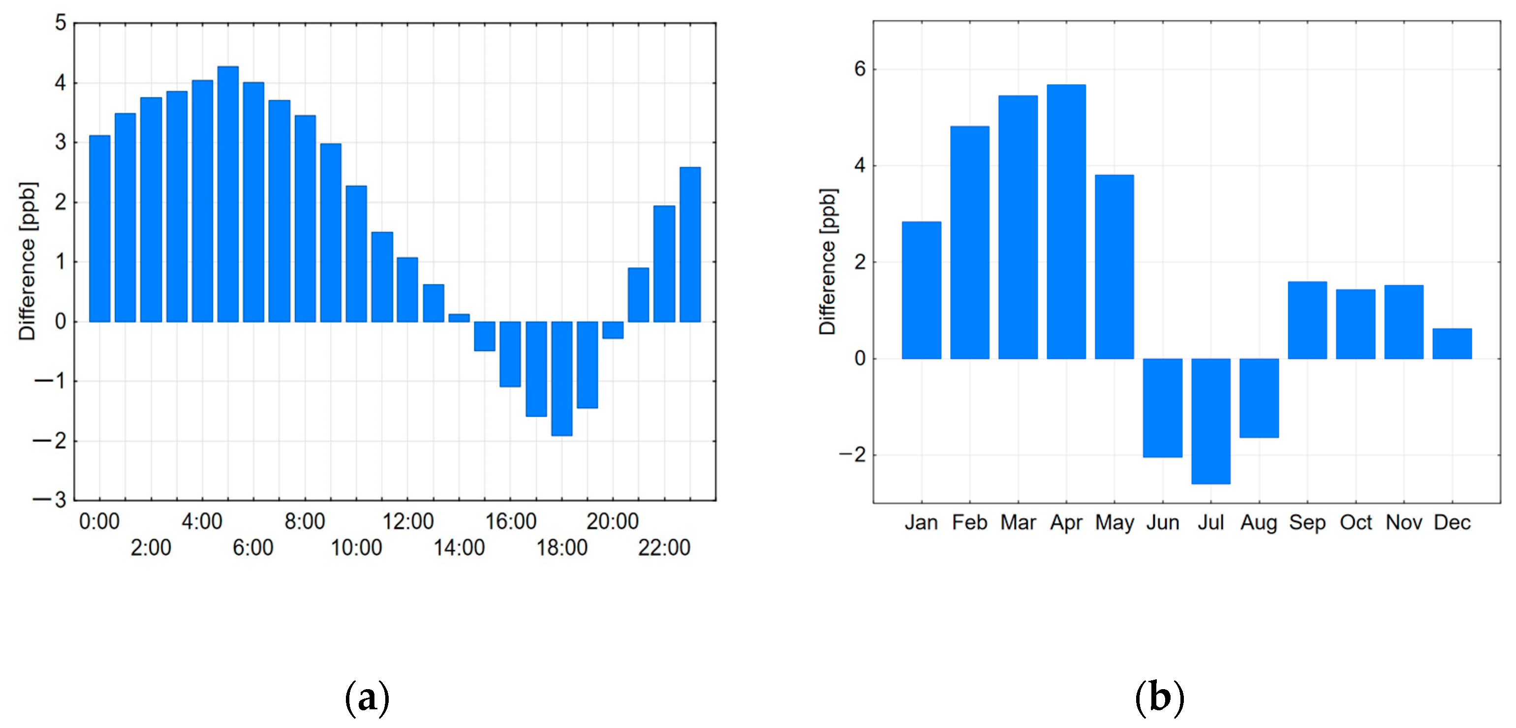
The rural-suburban surface O3 differences were examined for individual hours and months. Results show that the differences (rural minus suburban) are much higher during night and morning hours (Figure 5a) and during winter-spring months (Figure 5b). During the afternoons and evenings (from 15:00 to 20:00), greater surface O3 is noted in Racibórz station, similarly as during summer months (from June to August) which indicates the greater photochemical potential of surface O3 formation.
The fit of the hourly and monthly surface O3 values to a normal distribution was performed using the Shapiro-Wilk test (significance level: α = 0.05). The test was applied separately for all data from September 2018 to September 2021 separately for each hour during the day. The same test was performed for daily averaged values separately for each month (January–December) in the period 2018–2021. As the analyzed data were not normally distributed, the nonparametric U Mann-Whitney test was applied to find out whether the differences in surface O3 concentrations between hours and months were statistically significant.
The difference between surface O3 concentration in Belsk and Racibórz was statistically significant at a 95% confidence level for all hours, with the exception of hours between 13:00 and 16:00 and 20:00 and for months from January to May and for July.

3.2. Seasonal Cycle of Surface O3 Concentration from CAMS Simulations

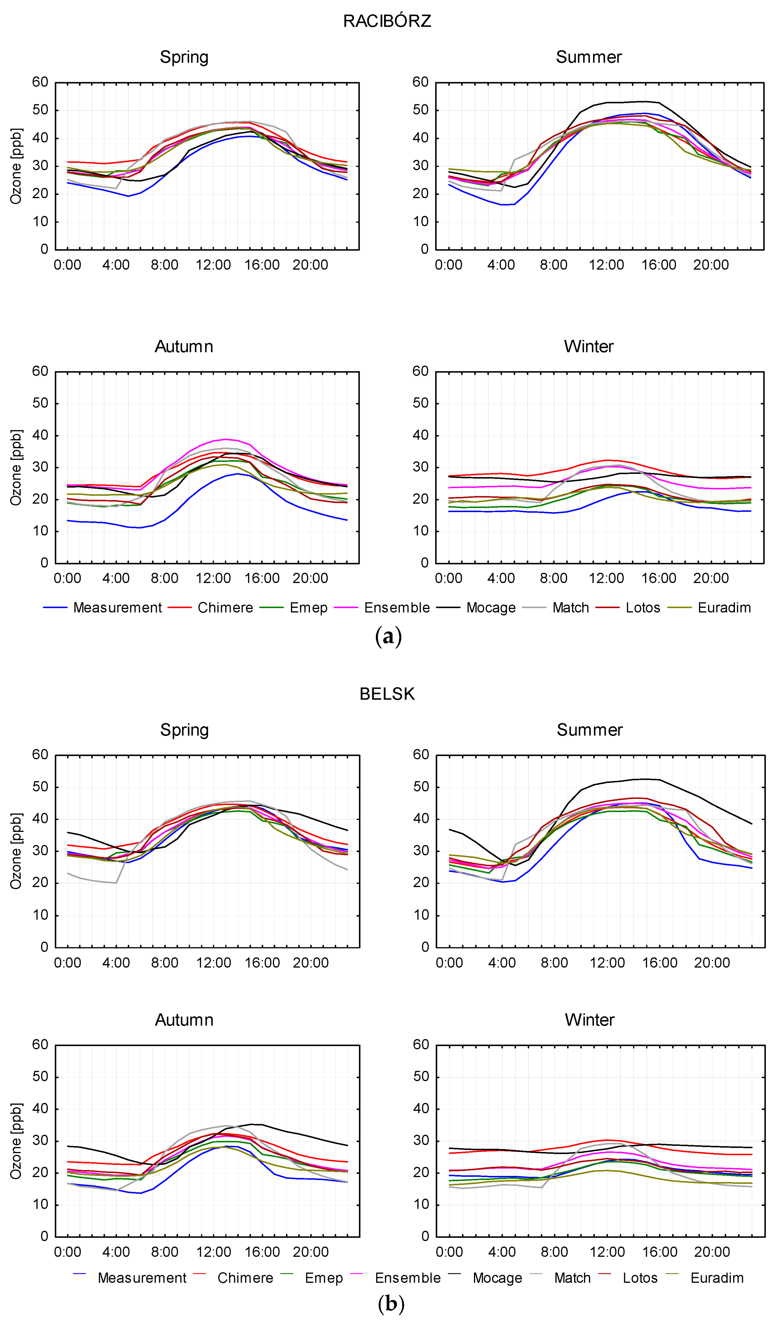
Figure 6 presents averaged daily variations of surface O3 from the measurements and CAMS forecasts for both stations for the period September 2018–September 2021. For each season, seven simulations: Chimere, Emep, Ensemble, Mocage, Match, Lotos, and Euradim were shown for both sites. Comparative analysis was performed separately for each location.
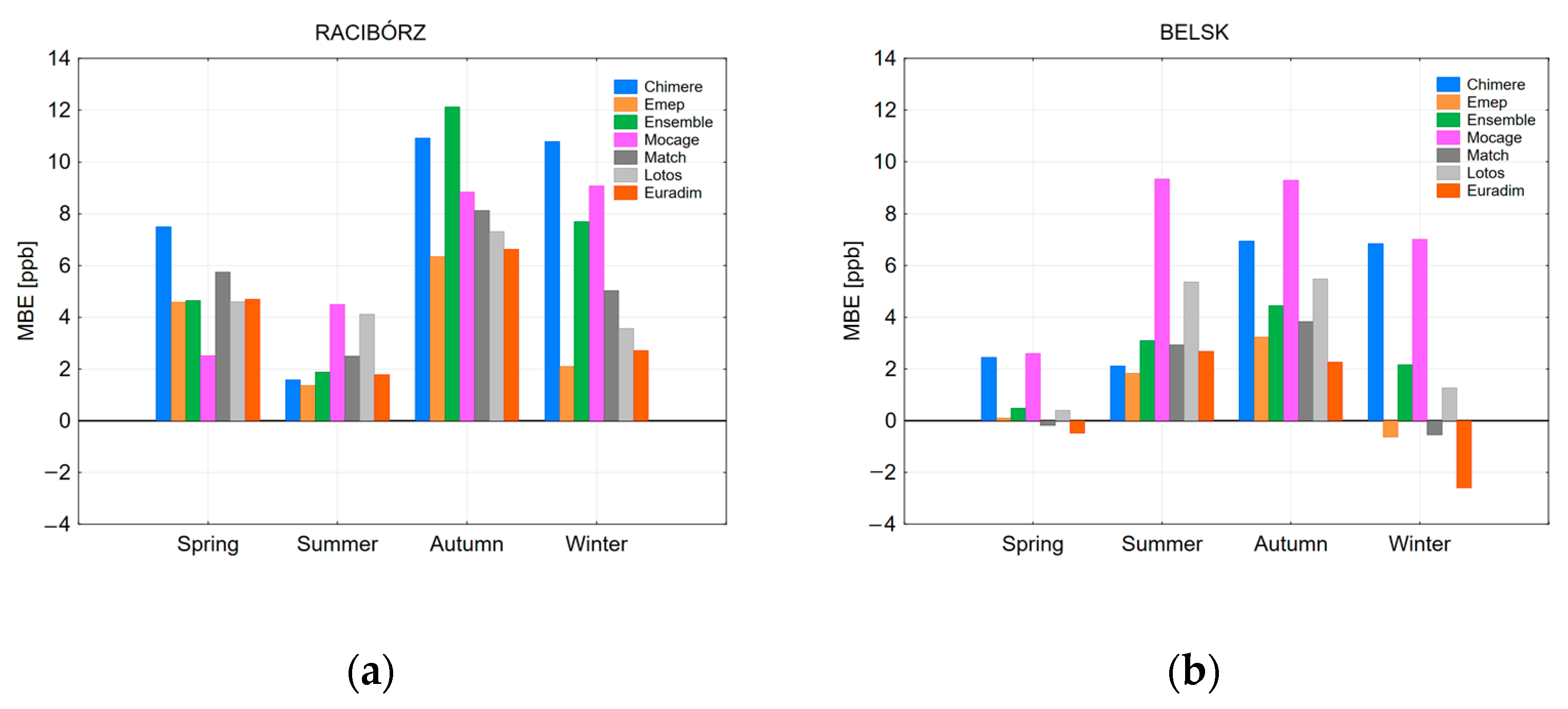
The mean differences between the CAMS forecasts and measured surface O3 are presented in Figure 7. All simulations show overestimation, especially during autumn and winter. In Belsk, the over- and under-estimations were slightly lower. Small under-estimations were noted during spring and winter for Emep, Match, and Euradim (up to 2.6 ppb). The simulations show differences not only in comparison with measurements but also when comparing CAMS pairs. More details on the CAMS-observation differences will be given in Section 3.3.
In order to determine whether the differences between CAMS forecast, and observations were statistically significant, the non-parametric U Manna-Whitney test was performed. The test was carried out using all hourly averaged data for individual seasons from 2018 to 2021 for each location. In almost all cases (with the exception of the spring season at Belsk for Emep), the differences between CAMS forecasts and observed surface O3 data were statistically significant.

3.3. Quality of CAMS Forecasts

CAMS model performance is determined by standard measures of goodness of fit of the model to the measurements, including coefficient of determination (R2), mean bias error (MBE) [ppb], mean absolute error (MAE) [ppb], and root mean squared error (RMSE) [ppb] (Table 2). These measures (so-called comparative statistics) are given by Equations (1)–(4), respectively.
R 2 = ( 1 n i = 1 n ( x i x ¯ ) ( y i   x ¯ ) SD x   SD y   )
MBE = 1 n i = 1 n ( y i x i )
MAE = 1 n i = 1 n | y i x i |
RMSE = 1 n i = 1 n ( y i x i ) 2
where: xi—observed variable, yi—predicted variable, x ¯ —mean of x variable, y ¯ —mean of y variable, SD x —standard deviation of observed variable, SD y —standard deviation of the predicted variable.
The R2 values show considerable variation depending on the season of the year. The highest values were found in summer and autumn, while the lowest were in winter. The R2 values in Racibórz ranged from 0.22 (Euradim-spring) to 0.70 (Ensemble-summer). For Belsk, these values were correspondingly lower, ranging from 0.22 (Lotos-winter) to 0.67 (Ensemble-autumn). All R2 values were statistically significant. The MBE values indicate a general tendency to overestimate observed values. The highest values were noted during autumn and winter. The MBE values in Racibórz varied between 1.37 ppb (Emep-summer) and 12.13 ppb (Ensemble-autumn). Lower values of MBE were noted in Belsk and ranged from 0.10 ppb (Emep-spring) to 9.34 (Mocage-summer). The MAE values in Racibórz ranged from 5.59 ppb (Emep-winter) to 12.54 ppb (Ensemble-autumn). For Belsk, these values were correspondingly lower and ranged from 5.01 ppb (Ensemble-spring) to 14.25 ppb (Mocage-summer). The RMSE values in Racibórz varied from 7.36 ppb (Emep-winter) to 16.18 ppb (Ensemble-autumn) while in Belsk from 6.30 ppb (Emep-winter) to 14.25 ppb (Mocage-Summer). The higher RMSE values compared with MAE values were noted for each season and for both locations, which indicates an appearance of large residual values. Both MAE and RMSE show the better statistical performance of CAMS forecasts in spring (Belsk) and summer (Racibórz).

3.4. Performance of MLR and ANN Models

Various models for predicting surface O3 are possible, ranging from the MLR model to sophisticated artificially intelligent ones such as XGBoost, based on many predictors containing chemical and weather components. Here we use two types of forecast model. i.e., MLR and ANN, which are adapted to a limited number of input variables available at the sites. The former aims to model the linear input-output relationship, and the latter one is to account for the possible nonlinearity effects between input variables and output.
Prediction of 1 h mean of surface O3 every 3 h from 0:00 GMT for each season of the year was based on observed meteorological data measured (every 3 h) at the stations. Using Statistica 12, ANN package, the models were developed for 2 independent sets of input data. The former one consisted of the following predictors: the hour of the day, temperature [°C], and relative humidity [%]. The latter one additionally takes into account: temperature 3 h back, relative humidity 3 h back, and surface O3 concentration 24 h back [ppb]. Particular data sets were implemented for the automatic network designer function. The input data set was divided into training (70%), test (15%), and validation (15%) subsets. Participants for each subset were selected randomly. Testing three-layer MLP with different functions of activation and different number of neurons in the hidden layer, the most appropriate topology of network structure was found. Table 3 presents the architecture of ANN for the validation subset used in the prediction.
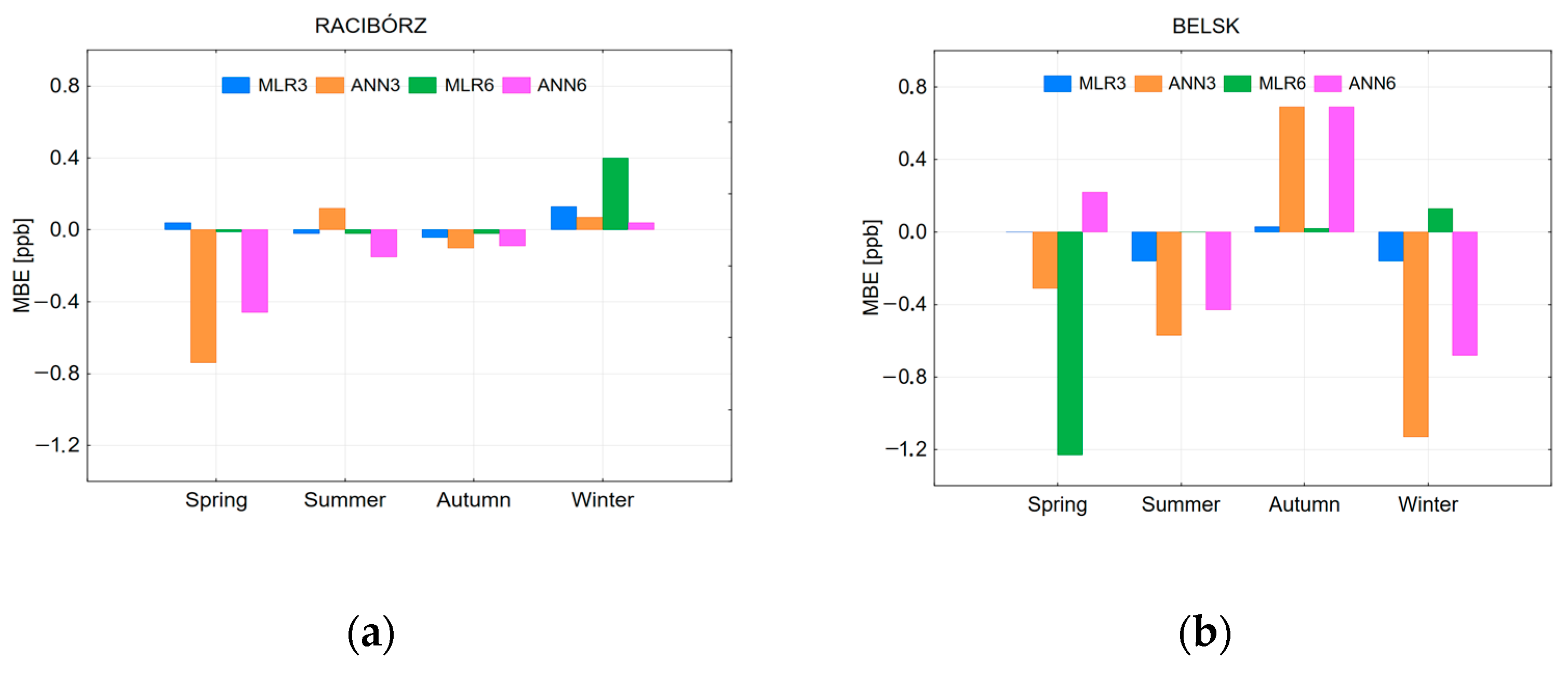
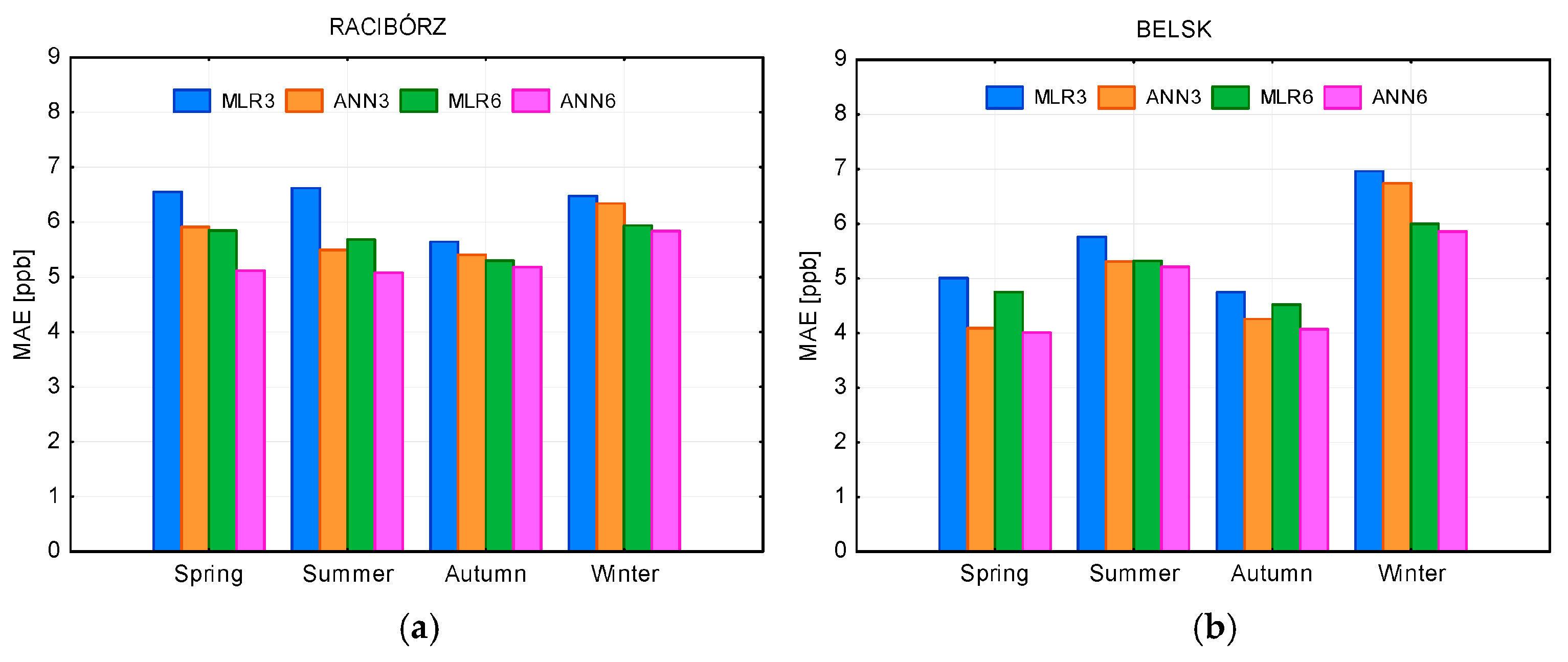
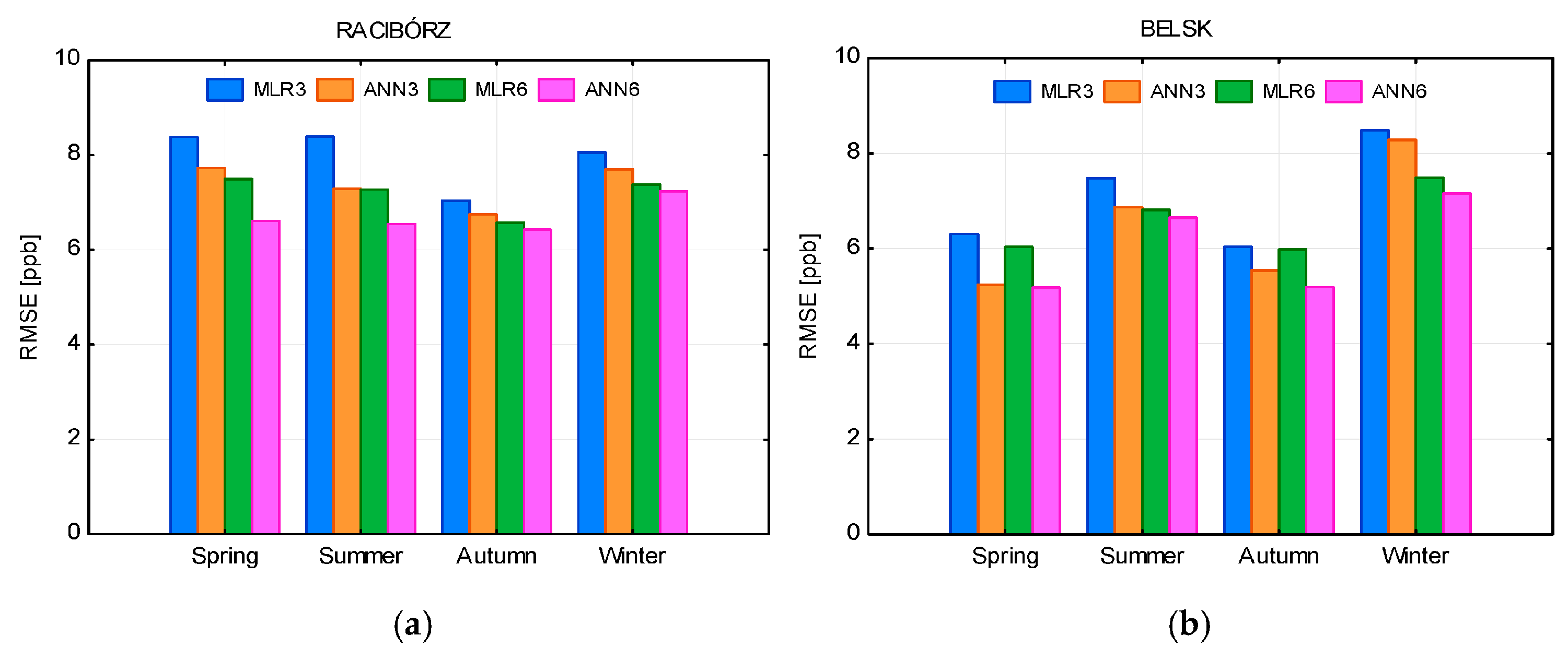
Depending on the number of input data sets, the best architecture of ANN models consisted of 3 or 6 neurons in the input layer, from 4 to 10 in the hidden layer, and 1 neuron in the output layer. The models used the gradient quasi-Newton BFGS (Broyden-Fletcher-Goldfarb-Shanno) learning algorithm. The selection of the best networks was performed considering the same statistical measures (evaluative statistics) used for quality checking of the CAMS forecasts (see Table 2). Table 4 presents the values of evaluative statistics using MLR and ANN for both sets of input data, for each season of the year separately for Racibórz and Belsk stations. Both kinds of models were developed based on two sets of input data, including three predictors (hour of the day, temperature, relative humidity) or six predictors (hour of the day, temperature, relative humidity, temperature 3 h back, relative humidity 3 h back, previous day’s surface O3 concentration). Performance indexes for ANN models were calculated for the validation data subset. The visual reference of results from Table 4, presenting the relative ranking of individual models, is shown in Figure 8, Figure 9, Figure 10 and Figure 11.
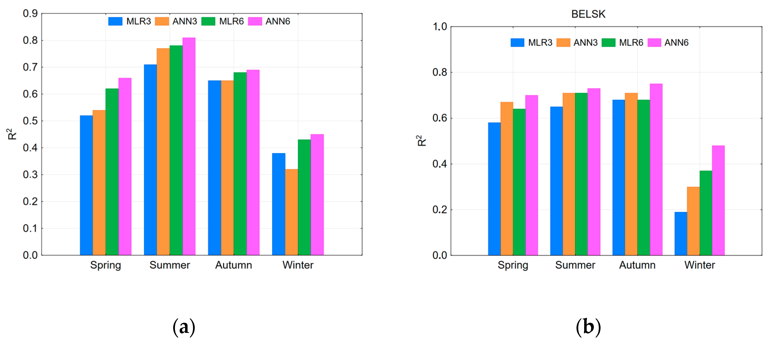
MLR model that was trained by a set of three input data (MLR3) explains up to 71% of the variance in surface O3 in Racibórz (summer) and up to 68% at Belsk (autumn). In turn, the ANN models trained by the same set of input data (ANN3) explains up to 77% in Racibórz (summer) and up to 71% at Belsk (summer and autumn). The use of a larger set of six input data results in improved model performance. The MLR6 model explains up to 78% in Racibórz and up to 71% at Belsk, while the ANN6 model explains up to 81% in Racibórz and up to 75% at Belsk. Generally, high R2 values are for summer and autumn but the lowest for winter. It’s worth noting that during summer, distinctly higher R2 values were noted for Racibórz station. During other seasons the R2 values between both stations were comparable.
The MBE values are small, ranging between −0.74 ppb (ANN3-spring) and 0.40 ppb (MLR6-winter) in Racibórz and between −1.23 ppb (MLR6-winter) and 0.69 ppb (ANN3-autumn) at Belsk. It shows great variation depending on the season and the kind of models. All models tend to slightly overestimate surface O3 concentrations. When comparing stations, higher absolute values of MBE were noted in Belsk.
Analyzing MLR3 models, the MAE value ranged between 5.64 ppb (autumn) and 6.62 ppb (summer) in Racibórz and between 4.75 ppb (autumn) and 6.96 ppb (winter) at Belsk. For ANN3 models, the MAE value ranged from 5.41 ppb (autumn) to 6.34 ppb (winter) in Racibórz and from 4.09 ppb (spring) to 6.74 ppb (winter) at Belsk. Addition of lagged ozone data and two lagged meteorological predictors reduced the MAE value by MLR6 models to 5.30 ppb (autumn) in Racibórz and to 4.52 ppb (autumn) at Belsk and of ANN6 models to 5.08 ppb (summer) in Racibórz and to 4.01 ppb (spring) at Belsk. For both models, the highest MAEs were noted for the winter months.
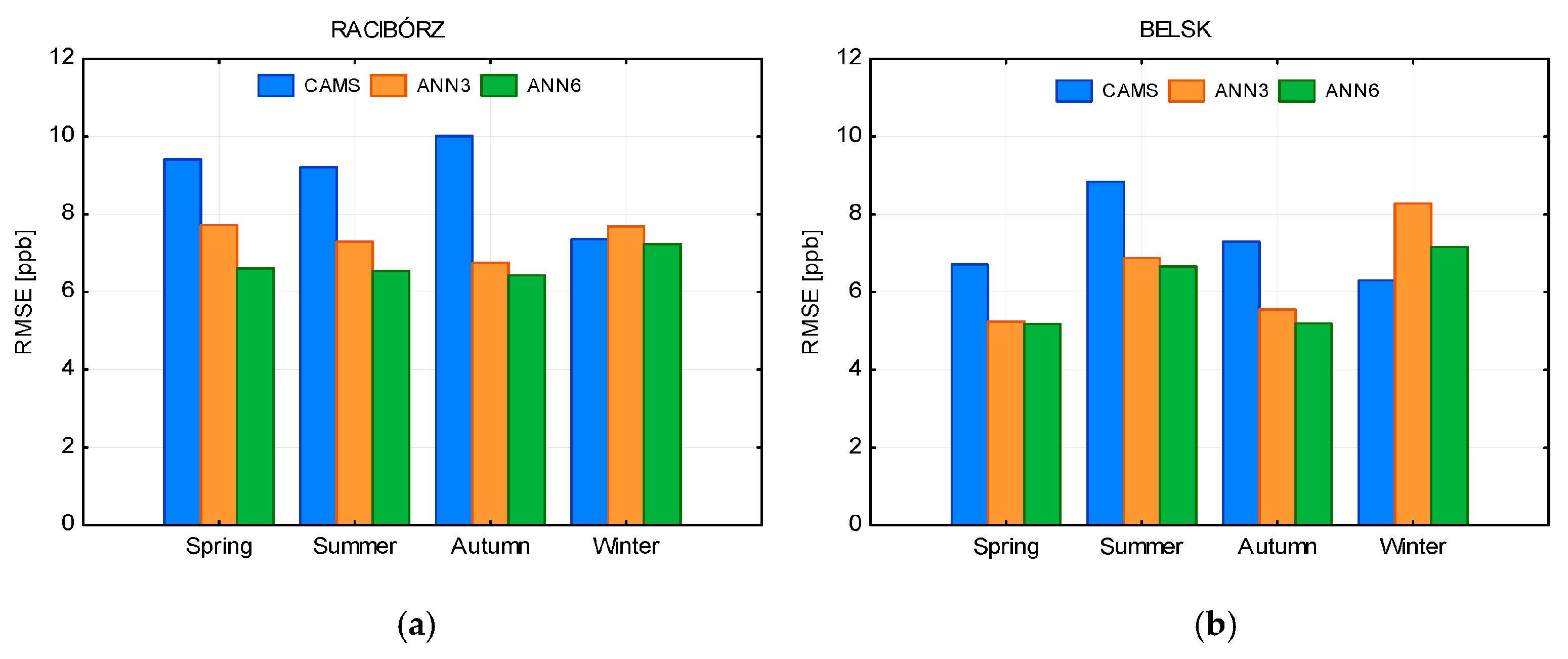
The results of RMSE follow a similar pattern to MAE, although its value in all cases is slightly higher than MAE because of higher sensitivity to outliers. For MLR3 models, trained with a set of three input data, RMSE ranged between 7.03 ppb (autumn) and 8.39 ppb (summer) in Racibórz and between 6.04 ppb (spring) and 8.49 ppb (winter) at Belsk. ANN3 models perform slightly better with RMSE between 6.75 ppb (autumn) and 7.69 ppb (winter) in Racibórz and between 5.24 ppb (spring) and 8.28 ppb (winter) in Belsk. Minimum RMSE for MLR6 models (trained with a set of 6 input data) were equal to 6.57 ppb (autumn) in Racibórz and 5.98 ppb (autumn) in Belsk. RMSE for ANN6 models reduced to 6.43 ppb (autumn) in Racibórz and to 5.18 ppb (spring) at Belsk.
Comparing model performance in terms of the number of input data (three or six), it appears that ANN, in all cases, is somewhat better than MLR. It seems that the inherent element of nonlinearity in ANN models provides a more accurate surface O3 forecast compared with MLR. The inclusion of additional input data, e.g., lagged surface O3 values (24 h back) and meteorological variables (temperature and relative humidity 3 h back), resulted in better performance of both kinds of models. However, improvement is slightly better for MLR than for ANN models.

3.5. Comparison of Performance of MLR and ANN with CAMS Simulations

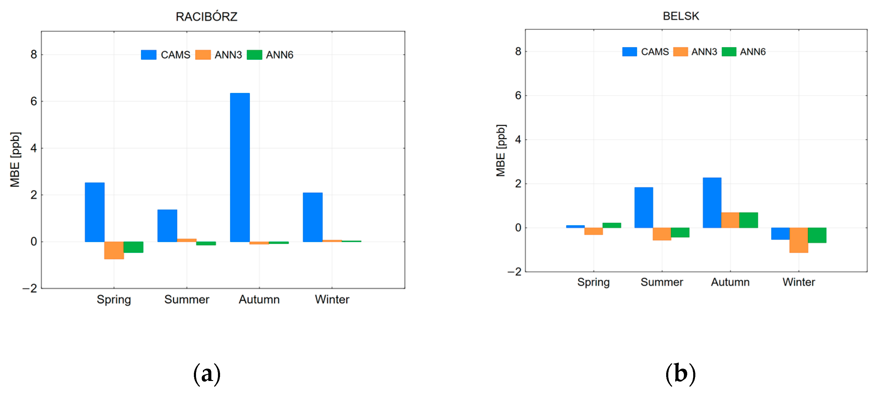
The architecture of the MLR and ANN model was built using the meteorological variable measured in stations. Figure 12, Figure 13, Figure 14 and Figure 15 present the results of the best CAMS forecast (blue), ANN3 (orange), and ANN6 (green) in terms of R2, MBE, MAE, and RMSE for Racibórz and Belsk stations. Depending on the season, the best CAMS forecast was: Emep (50% of cases), Ensemble (40%), Mocage (3.3%), Match (3.3%), and Euradim (3.3%).
Comparing the performance of these three models in terms of R2 value, it can be stated that for spring, summer, and autumn, the R2 was higher for ANN3 and ANN6 models, while for winter, the CAMS simulation (Emep) was better. MBE values indicate the over-estimation by CAMS simulations for both locations during all seasons, with the exception of winter at Belsk, when small (below 1 ppb) under-estimation by Match forecast was recorded. In terms of MAE and RMSE, for spring, summer, and autumn, the forecast by ANN3 and ANN6 were better than those taken from the best CAMS forecast. In the winter season, the CAMS forecast reached a better fit for the measured data. It suggests that ANN with the MLP structure could be an effective tool supporting the prediction of surface O3 during spring-summer-autumn when there is a real risk of episodes of high surface O3.

4. Discussion

This study presents the performance of MLR and ANN (with an MLP approach) in forecasting surface O3 in rural and suburban locations in Poland. Both models were built using two separate sets of input data containing a limited number (three or six) of predictors. Because surface O3 is mainly formed by photochemical reactions, the combination of basic meteorological parameters (temperature and relative humidity) with additional variables, including an hour of the day and lagged surface O3 data, were used as an explanatory variable. Similarly, to Yi and Prybutok [37], Comrie [38], Spellmann [39], Gardner and Dorling [40], Sousa et al. [41], and Yu et al. [43], the results showed that the use of ANN models performs better than linear models what indicate possible interactions and non-linear relationships between predictors and surface O3. MLR explained up to 78% of the variance in surface O3 in Racibórz and up to 71% in Belsk, while the ANN model explained up to 81% in Racibórz and up to 75% at Belsk.
The use of three additional input data, including the surface O3 concentration from the previous day, improves the quality of the estimation of both models. The gain is up to 18 percentage points for MLR and up to 13 percentage points for ANN models). It is worth noting that statistical models presented in this work used only the basic set of parameters determining surface O3 formation. Other meteorological parameters or in-situ surface O3 precursor concentrations (NOx, VOC) were not included in the presented analysis. We can suggest that the inclusion of these predictors into a set of input data might further improve the results of modeling. MLR and ANN models provided better forecasts for the rural station (Belsk). It is probably related to the greater uniformity and representativeness of non-urban areas.
Surface O3 forecasts using ANN models were also performed based on CAMS meteorological data. The R2 values ranged up to 0.61 in Racibórz (summer) and up to 0.52 in Belsk (autumn), while RMSE values ranged up to 10.35 ppb in both locations. These results, in most cases, were better compared to results obtained by CAMS surface O3 forecasts but worse when compared with results obtained using measured meteorological data (R2 up to 0.81, RMSE up to 6.43 in Racibórz and R2 up to 0.75 and RMSE up to 5.18 ppb in Belsk). The performance of statistical models depends crucially on the quality of the forecast of the meteorological field. Using observed parameters is equivalent to using the perfect meteorological forecast.
Furthermore, this study investigates the efficiency of surface O3 prediction obtained by selected CAMS simulations. Statistical analysis of differences between measurements and CAMS forecasts showed significant overestimations of CAMS results, especially for Racibórz during the autumn season. Comparative analysis indicates better performance of MLR and ANN models trained by a set of six input data compared to CAMS simulations for both locations for all seasons with the exception of winter. Forecasts by MLR and ANN for the cold part of the year are less accurate, with an R2 value below 0.5 for both models. It is worth noticing that ANN, with three predictors (temperature, relative humidity, and the hour of the day) provided an even better forecast (except winter) than the best CAMS forecast. Such a simple forecast can be used for any place in Poland, and measurements of surface O3 are not necessary for the such forecast.
The results of the machine learning algorithm using different categories of predictors (including CAMS surface O3 simulations) for predicting surface O3 in Munich (Germany) were presented in the work of Balamurugan et al. [60]. In contrast to the present study, the results concerned the diurnal maximum (from 13:00 to 14:00) of surface O3 for the whole year without division into seasons. The Extreme Gradient Boosting (XGBoost) approach trained only on meteorology parameters (temperature, relative humidity, boundary layer height, wind speed, and wind direction) explained 77% of the variance of measured surface O3 with RMSE value ~8 ppb. These results are comparable with MLR6 and ANN3 achieved in the present study. XGBoost trained only on CAMS data showed worse performance. It explained 75% of the variance in surface O3 with RMSE ~8.5 ppb. The results obtained for the best CAMS simulations in the present study explained up to 70% of the variance in surface O3 with RMSE equal to 9.21 ppb (Racibórz—Summer). It is worth noticing that the performance of our statistical models in all seasons except winter was clearly better than CAMS alternatives (see Figure 11, Figure 12, Figure 13 and Figure 14). Balamurugan et al. [60] found that the differences between R2 and RMSE for their models based on meteorology and CAMS O3 forecasts were rather marginal.

5. Conclusions

Surface ozone has been measured in the Polish national network involving monitoring of other gaseous components important for the determination of air quality. This study shows that effective forecasting of surface ozone for rural and suburban sites in Poland is possible using only surface O3, temperature, and humidity. Monitoring of these weather variables can be carried out even by simplified weather stations, i.e., with no wind measurements. This low-cost configuration increases the number of locations providing short-term surface O3 predictions important to local communities.

Author Contributions

Conceptualization, I.P. and A.F.; methodology, I.P. and A.F.; preparation of data, J.J., A.P., K.K. and A.F.; statistical analysis; I.P.; writing—original draft preparation, I.P. and A.F.; writing—review and editing, A.P. and J.J.; preparation of figures, I.P.; supervision, A.P. and J.J. All authors have read and agreed to the published version of the manuscript.

Funding

This work was funded by the National Science Center in Poland under grant UMO-2017/25/B/ST10/01650. This work was partially founded by the Chief Inspectorate of Environmental Protection, GIOŚ/19/2021/DMŚ/NFOŚ. Observatory activities at Belsk and Racibórz were supported by Polish Ministry of Education and Science (Decision No. 13/E-41/SPUB/SP/2020).

Institutional Review Board Statement

Not applicable.

Informed Consent Statement

Not applicable.

Data Availability Statement

The observed surface O3 from Racibórz and Belsk data is available on the IG PAS Data Portal (https://dataportal.igf.edu.pl/organization/ atmospheric-physics) (accessed on 25 March 2023). The surface O3 CAMS data is available through the website https://ads.atmosphere.copernicus.eu/cdsapp#!/dataset/cams-europe-air-quality-forecasts?tab=form (accessed on 25 March 2023). The temperature and relative humidity CAMS data are available through the website https://ads.atmosphere.copernicus.eu/cdsapp#!/dataset/cams-global-atmospheric-composition-forecasts?tab=form (accessed on 25 March 2023).

Conflicts of Interest

The authors declare no conflict of interest.

References

  1. Ramsey, N.R.; Klein, P.M.; Moore, B. The Impact of Meteorological Parameters on Urban Air Quality. Atmos. Environ. 2014, 86, 58–67. [Google Scholar] [CrossRef]
  2. Crutzen, P. A Discussion of the Chemistry of Some Minor Constituents in the Stratosphere and Troposphere; Birkhg.user Verlag: Basel, Switzerland, Pure and Applied Geophysics; 1973; Volume 106. [Google Scholar]
  3. Seinfeld, J.H. Urban Air Pollution: State of the Science. Science 1989, 243, 745–752. [Google Scholar] [CrossRef]
  4. Jacob, D.J. Heterogeneous Chemistry and Tropospheric Ozone. Atmos. Environ. 2000, 34, 2131–2159. [Google Scholar] [CrossRef]
  5. Edwin, F. Danielsen Stratospheric-Tropospheric Exchange Based on Radioactivity, Ozone and Potential Vorticity. J. Atmos. Sci. 1968, 25, 502–518. [Google Scholar]
  6. Stohl, A. Stratosphere-Troposphere Exchange: A Review, and What We Have Learned from STACCATO. J. Geophys. Res. 2003, 108, 8516. [Google Scholar] [CrossRef]
  7. Hov, Ö.; Hesstvedt, E.; Isaksen, I.S.A. Long-Range Transport of Tropospheric Ozone. Nature 1978, 273, 341–344. [Google Scholar] [CrossRef]
  8. Gosten, H.; Heinrich, N.; Monnich, E.; Sprung, D.; Weppner, J.; Bakr Ramadan, A.; M Ezz El-din, M.R.; Ahmed, D.M.; Y Hassan, G.K. ON-line measurements of ozone surface fluxes: Part II. surface-level ozone fluxes onto the sahara desert. Atmos. Environ. 1996, 30, 911–918. [Google Scholar] [CrossRef]
  9. Atkinson, R. Atmospheric Chemistry of VOCs and NOx. Atmos. Environ. 2000, 34, 2063–2101. [Google Scholar] [CrossRef]
  10. Sillman, S. The Relation between Ozone, NOx and Hydrocarbons in Urban and Polluted Rural Environments. Atmos. Environ. 1999, 33, 1821–1845. [Google Scholar] [CrossRef]
  11. Dueñas, C.; Fernández, M.C.; Cañete, S.; Carretero, J.; Liger, E. Analyses of Ozone in Urban and Rural Sites in Málaga (Spain). Chemosphere 2004, 56, 631–639. [Google Scholar] [CrossRef]
  12. Han, J.; Kim, H.; Lee, M.; Kim, S.; Kim, S. Photochemical Air Pollution of Seoul in the Last Three Decades. J. Korean Soc. Atmos. Environ. 2013, 29, 390–406. [Google Scholar] [CrossRef] [Green Version]
  13. Pawlak, I.; Jarosławski, J. The Influence of Selected Meteorological Parameters on the Concentration of Surface Ozone in the Central Region of Poland. Atmosphere Ocean 2015, 53, 126–139. [Google Scholar] [CrossRef]
  14. Crutzen, P.J.; Zimmermann, P.H. The Changing Photochemistry of the Troposphere. Tellus A 1991, 43, 136–151. [Google Scholar] [CrossRef]
  15. Forster, P.; Alterskjaer, K.; Smith, C.; Colman, R.; Damon Matthews, H.; Ramaswamy, V.; Storelvmo, T.; Armour, K.; Collins, W.; Dufresne, J.; et al. SPM 923 7 Coordinating Lead Authors: Contributing Authors: Review Editors: Chapter Scientists: The Earth’s Energy Budget, Climate Feedbacks and Climate Sensitivity; Cambridge University Press: Cambridge, UK; New York, NY, USA, 2021; pp. 923–1054. [Google Scholar] [CrossRef]
  16. Sillman, S. Tropospheric Ozone and Photochemical Smog. In Treatise on Geochemistry; Elsevier: Amsterdam, The Netherlands, 2003; pp. 407–431. [Google Scholar]
  17. Malley, C.S.; Heal, M.R.; Mills, G.; Braban, C.F. Trends and Drivers of Ozone Human Health and Vegetation Impact Metrics from UK EMEP Supersite Measurements (1990–2013). Atmos. Chem. Phys. 2015, 15, 4025–4042. [Google Scholar] [CrossRef] [Green Version]
  18. Liu, X.; Tai, A.P.K.; Fung, K.M. Responses of Surface Ozone to Future Agricultural Ammonia Emissions and Subsequent Nitrogen Deposition through Terrestrial Ecosystem Changes. Atmos. Chem. Phys. 2021, 21, 17743–17758. [Google Scholar] [CrossRef]
  19. Wilson, A.; Rappold, A.G.; Neas, L.M.; Reich, B.J. Modeling the Effect of Temperature on Ozone-Related Mortality. Ann. Appl. Stat. 2014, 8, 1728–1749. [Google Scholar] [CrossRef]
  20. Logan, J.A. Tropospheric Ozone: Seasonal Behavior, Trends, and Anthropogenic Influence. J. Geophys.Res. Atmos. 1985, 90, 10463–10482. [Google Scholar] [CrossRef]
  21. Seinfeld, J.H.; Pandis, S.N. Atmospheric Chemistry and Physics: From Air Pollution to Climate Change, 2nd ed.; John Wiley & Sons: New York, NY, USA, 2006. [Google Scholar]
  22. Sillman, S.; Samson, P.J. Impact of Temperature on Oxidant Photochemistry in Urban, Polluted Rural and Remote Environments. J. Geophys. Res. 1995, 100, 11497. [Google Scholar] [CrossRef]
  23. Arya, S.P. Air Pollution Meteorology and Dispersion; Oxford University Press: Oxford, UK, 1999. [Google Scholar]
  24. Lelieveld, J.; Crutzen, P.J. The Role of Clouds in Tropospheric Photochemistry. J. Atmos. Chem. 1991, 12, 229–267. [Google Scholar] [CrossRef]
  25. Zhang, L.; Brook, J.R.; Vet, R. A Revised Parameterization for Gaseous Dry Deposition in Air-Quality Models. Atmos. Chem. Phys. 2003, 3, 2067–2082. [Google Scholar] [CrossRef] [Green Version]
  26. Hodnebrog, Ø.; Solberg, S.; Stordal, F.; Svendby, T.M.; Simpson, D.; Gauss, M.; Hilboll, A.; Pfister, G.G.; Turquety, S.; Richter, A.; et al. Impact of Forest Fires, Biogenic Emissions and High Temperatures on the Elevated Eastern Mediterranean Ozone Levels during the Hot Summer of 2007. Atmos. Chem. Phys. 2012, 12, 8727–8750. [Google Scholar] [CrossRef] [Green Version]
  27. Derwent-, R.G.; Jenkin, M.E.; Saundersm, S.M.; Pillingm, M.J. Photochemical ozone creation potentials for organic compounds in northwest europe calculated with a master chemical mechanism. Atmos. Environ. 1998, 32, 2429–2441. [Google Scholar] [CrossRef]
  28. Tarasova, O.A.; Karpetchko, A.Y. Accounting for Local Meteorological Effects in the Ozone Time-Series of Lovozero (Kola Peninsula). Atmos. Chem. Phys. 2003, 3, 941–949. [Google Scholar] [CrossRef] [Green Version]
  29. Camalier, L.; Cox, W.; Dolwick, P. The Effects of Meteorology on Ozone in Urban Areas and Their Use in Assessing Ozone Trends. Atmos. Environ. 2007, 41, 7127–7137. [Google Scholar] [CrossRef]
  30. Vautard, R.; Beekmann, M.; Roux, J.; Gombert, D. Validation of a Hybrid Forecasting System for the Ozone Concentrations over the Paris Area. Atmos. Environ. 2001, 35, 2449–2461. [Google Scholar] [CrossRef]
  31. Vautard, R.; Moran, M.D.; Solazzo, E.; Gilliam, R.C.; Matthias, V.; Bianconi, R.; Chemel, C.; Ferreira, J.; Geyer, B.; Hansen, A.B.; et al. Evaluation of the Meteorological Forcing Used for the Air Quality Model Evaluation International Initiative (AQMEII) Air Quality Simulations. Atmos. Environ. 2012, 53, 15–37. [Google Scholar] [CrossRef] [Green Version]
  32. Verma, N.; Lakhani, A.; Maharaj Kumari, K. High Ozone Episodes at a Semi-Urban Site in India: Photochemical Generation and Transport. Atmos. Res. 2017, 197, 232–243. [Google Scholar] [CrossRef]
  33. Lou, S.; Liao, H.; Yang, Y.; Mu, Q. Simulation of the Interannual Variations of Tropospheric Ozone over China: Roles of Variations in Meteorological Parameters and Anthropogenic Emissions. Atmos. Environ. 2015, 122, 839–851. [Google Scholar] [CrossRef]
  34. Hu, J.; Chen, J.; Ying, Q.; Zhang, H. One-Year Simulation of Ozone and Particulate Matter in China Using WRF/CMAQ Modeling System. Atmos. Chem. Phys. 2016, 16, 10333–10350. [Google Scholar] [CrossRef] [Green Version]
  35. Singh, J.; Singh, N.; Ojha, N.; Sharma, A.; Pozzer, A.; Kiran Kumar, N.; Rajeev, K.; Gunthe, S.S.; Rao Kotamarthi, V. Effects of Spatial Resolution on WRF v3.8.1 Simulated Meteorology over the Central Himalaya. Geosci. Model Dev. 2021, 14, 1427–1443. [Google Scholar] [CrossRef]
  36. Sharma, A.; Ojha, N.; Pozzer, A.; Mar, K.A.; Beig, G.; Lelieveld, J.; Gunthe, S.S. WRF-Chem Simulated Surface Ozone over South Asia during the Pre-Monsoon: Effects of Emission Inventories and Chemical Mechanisms. Atmos. Chem. Phys. 2017, 17, 14393–14413. [Google Scholar] [CrossRef] [Green Version]
  37. Yi, J.; Prybutok, V.R. A neural network model forecasting for prediction of daily maximum ozone concentration in an industrialized urban area. Environ. Pollut. 1996, 92, 349–357. [Google Scholar] [CrossRef]
  38. Comrie, A.C. Comparing Neural Networks and Regression Models for Ozone Forecasting. J. Air Waste Manag. Assoc. 1997, 47, 653–663. [Google Scholar] [CrossRef]
  39. Spellman, G. An Application of Artificial Neural Networks to the Prediction of Surface Ozone Concentrations in the United Kingdom. Appl. Geogr. 1999, 19, 123–136. [Google Scholar] [CrossRef]
  40. Gardner, M.W.; Dorling, S.R. Statistical Surface Ozone Models: An Improved Methodology to Account for Non-Linear Behaviour. Atmos. Environ. 2000, 34, 21–34. [Google Scholar] [CrossRef]
  41. Sousa, S.I.V.; Martins, F.G.; Alvim-Ferraz, M.C.M.; Pereira, M.C. Multiple Linear Regression and Artificial Neural Networks Based on Principal Components to Predict Ozone Concentrations. Environ. Model. Softw. 2007, 22, 97–103. [Google Scholar] [CrossRef]
  42. Capilla, C. Prediction of Hourly Ozone Concentrations with Multiple Regression and Multilayer Perceptron Models. Int. J. Sustain. Dev. Plan. 2016, 11, 558–565. [Google Scholar] [CrossRef] [Green Version]
  43. Yu, J.; Xu, L.; Gao, S.; Chen, L.; Sun, Y.; Mao, J.; Zhang, H. Establishment of a Combined Model for Ozone Concentration Simulation with Stepwise Regression Analysis and Artificial Neural Network. Atmosphere 2022, 13, 1371. [Google Scholar] [CrossRef]
  44. Freeman, B.S.; Taylor, G.; Gharabaghi, B.; Thé, J. Forecasting Air Quality Time Series Using Deep Learning. J. Air Waste Manag. Assoc. 2018, 68, 866–886. [Google Scholar] [CrossRef] [Green Version]
  45. Ko, K.; Cho, S.; Rao, R.R. Machine-Learning-Based Near-Surface Ozone Forecasting Model with Planetary Boundary Layer Information. Sensors 2022, 22, 7864. [Google Scholar] [CrossRef]
  46. Oufdou, H.; Bellanger, L.; Bergam, A.; Khomsi, K. Forecasting Daily of Surface Ozone Concentration in the Grand Casablanca Region Using Parametric and Nonparametric Statistical Models. Atmosphere 2021, 12, 666. [Google Scholar] [CrossRef]
  47. Jia, P.; Cao, N.; Yang, S. Real-Time Hourly Ozone Prediction System for Yangtze River Delta Area Using Attention Based on a Sequence to Sequence Model. Atmos. Environ. 2021, 244, 117917. [Google Scholar] [CrossRef]
  48. Juarez, E.K.; Petersen, M.R. A Comparison of Machine Learning Methods to Forecast Tropospheric Ozone Levels in Delhi. Atmosphere 2022, 13, 46. [Google Scholar] [CrossRef]
  49. Colette, A.; Andersson, C.; Manders, A.; Mar, K.; Mircea, M.; Pay, M.T.; Raffort, V.; Tsyro, S.; Cuvelier, C.; Adani, M.; et al. EURODELTA-Trends, a Multi-Model Experiment of Air Quality Hindcast in Europe over 1990–2010. Geosci. Model Dev. 2017, 10, 3255–3276. [Google Scholar] [CrossRef] [Green Version]
  50. Derwent, R.G.; Davies, T.J. Modelling the Impact of NOx or Hydrocarbon Control on Photochemical Ozone in Europe. Atmos. Environ. 1994, 28, 2039–2052. [Google Scholar] [CrossRef]
  51. Pavón-Domínguez, P.; Jiménez-Hornero, F.J.; Gutiérrez de Ravé, E. Proposal for Estimating Ground-Level Ozone Concentrations at Urban Areas Based on Multivariate Statistical Methods. Atmos. Environ. 2014, 90, 59–70. [Google Scholar] [CrossRef]
  52. Hashim, N.M.; Noor, N.M.; Ul-Saufie, A.Z.; Sandu, A.V.; Vizureanu, P.; Deák, G.; Kheimi, M. Forecasting Daytime Ground-Level Ozone Concentration in Urbanized Areas of Malaysia Using Predictive Models. Sustainability 2022, 14, 7936. [Google Scholar] [CrossRef]
  53. Silva, R.C.V.; Pires, J.C.M. Surface Ozone Pollution: Trends, Meteorological Influences, and Chemical Precursors in Portugal. Sustainability 2022, 14, 2383. [Google Scholar] [CrossRef]
  54. Gardner, M.W.; Dorling, S.R. Artificial neural networks (the multilayer perceptron)—A review of applications in the atmospheric sciences . Atmos. Environ. 1998, 32, 2627–2636. [Google Scholar]
  55. Lal, S.; Naja, M.; Subbaraya, B.H. Seasonal Variations in Surface Ozone and Its Precursors over an Urban Site in India. Atmospheric Environ. 2000, 34, 2713–2724. [Google Scholar] [CrossRef]
  56. Eliasson, I.; Thorsson, S.; Andersson-Sköld, Y. Summer Nocturnal Ozone Maxima in Göteborg, Sweden. Atmos. Environ. 2003, 37, 2615–2627. [Google Scholar] [CrossRef]
  57. Murphy, J.G.; Day, D.A.; Cleary, P.A.; Wooldridge, P.J.; Millet, D.B.; Goldstein, A.H.; Cohen, R.C. The Weekend Effect within and Downwind of Sacramento-Part 1: Observations of Ozone, Nitrogen Oxides, and VOC Reactivity. Atmos. Chem. Phys. 2007, 7, 5327–5339. [Google Scholar] [CrossRef] [Green Version]
  58. Hakola, H.; Joffre, S.; Lättilä, H.; Taalas, P. Transport, Formation and Sink Processes behind Surface Ozone Variability in North European Conditions. Atmos. Environ. Part A. Gen. Top. 1991, 25, 1437–1447. [Google Scholar] [CrossRef]
  59. Hsu, J.; Prather, M.J. Stratospheric Variability and Tropospheric Ozone. J. Geophys. Res. Atmos. 2009, 114, D06102. [Google Scholar] [CrossRef]
  60. Balamurugan, V.; Balamurugan, V.; Chen, J. Importance of Ozone Precursors Information in Modelling Urban Surface Ozone Variability Using Machine Learning Algorithm. Sci. Rep. 2022, 12, 5646. [Google Scholar] [CrossRef] [PubMed]
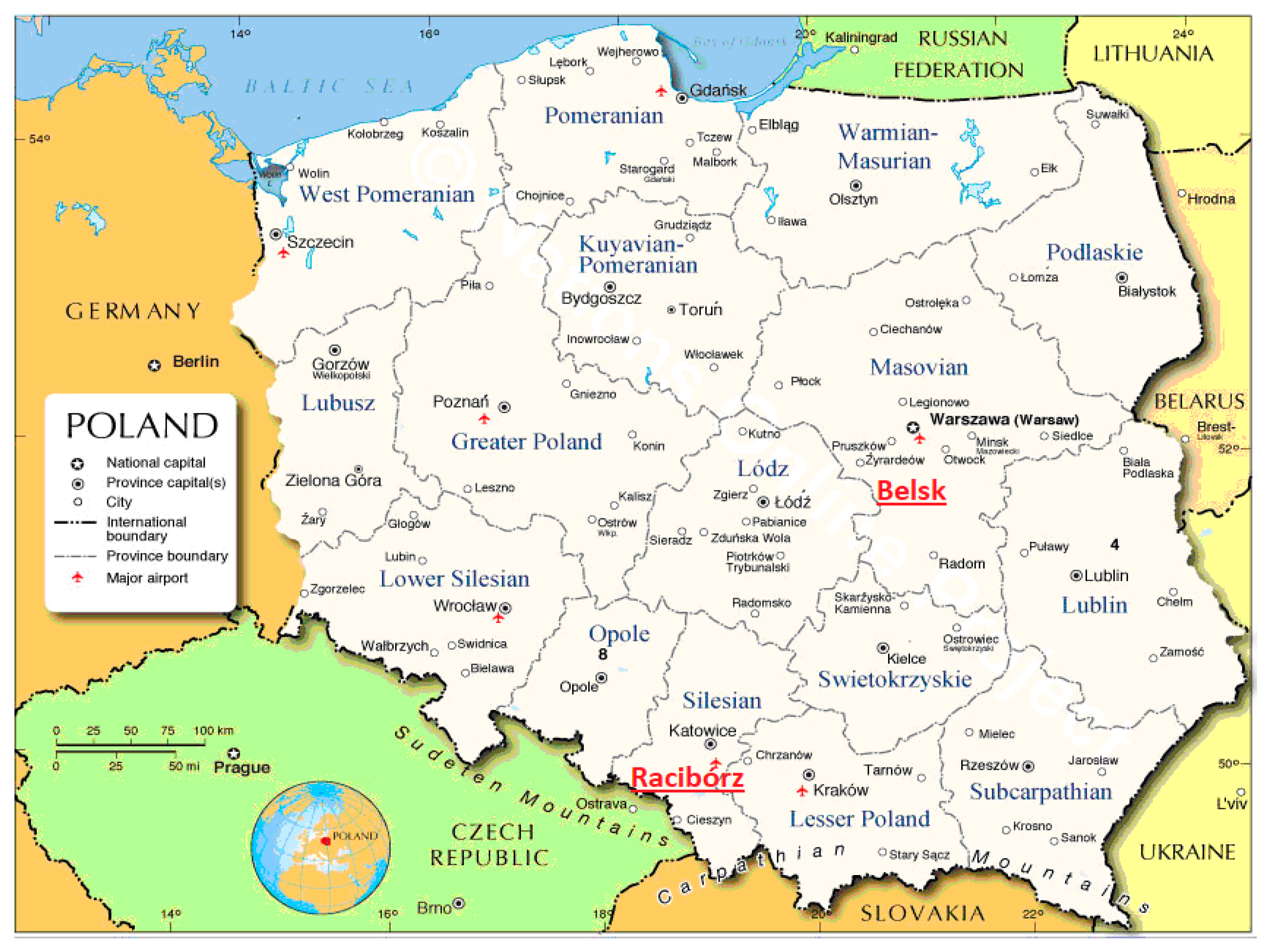
Figure 1. Location of the stations considered in the study. (source: nationsonline.org).
Atmosphere 14 00670 g001
Figure 2. Monthly averaged values of temperature [°C] and relative humidity [%] in Racibórz (a) and Belsk (b) for the period 2018–2021. Points display the mean value; the box shows the range: mean ± 1 standard deviation.
Atmosphere 14 00670 g002
Figure 3. Mean daily course of surface O3 from observations for the period from 2018 to 2021 in Racibórz (a) and at Belsk (b). The point shows the mean value, and the box displays the range: mean ± 1 standard deviation.
Atmosphere 14 00670 g003
Figure 4. Monthly average surface O3 concentrations in Racibórz (a) and at Belsk (b) for the period September 2018–September 2021. The point displays the mean value; the box shows the range: mean ± 1 standard deviation.
Atmosphere 14 00670 g004
Figure 5. The differences between surface O3 measured at Belsk and Racibórz (ppb), from 2018 to 2021, for diurnal (a) and monthly (b) scales.
Atmosphere 14 00670 g005
Figure 6. Time series of diurnal variation of surface O3 concentration for each season at Racibórz (a) and Belsk (b) station for the period 2018–2021. Colors of lines: blue-measurement, red-Chimere, dark green-Emep, pink-Ensemble, black-Mocage, light grey-Match, brown-Lotos, light green-Euradim.
Atmosphere 14 00670 g006
Figure 7. Mean bias error (see Equation (2) for definition), CAMS forecasts minus observed surface O3, for the period 2018–2021, separately for each season for Racibórz (a) and Belsk (b) station.
Atmosphere 14 00670 g007
Figure 8. Coefficient of determination (R2) for Racibórz (a) and Belsk (b) by model and season. MLR3—MLR based on a set of 3 input data, ANN3—ANN based on a set of 3 input data, MLR6—MLR based on a set of 6 input data, ANN6—ANN based on a set of 6 input data.
Atmosphere 14 00670 g008
Figure 9. The same as Figure 8 but for mean bias error (MBE) for Racibórz (a) and Belsk (b).
Atmosphere 14 00670 g009
Figure 10. The same as Figure 8 but for mean absolute error (MAE) for Racibórz (a) and Belsk (b).
Atmosphere 14 00670 g010
Figure 11. The same as Figure 8 but for root mean square error (RMSE) for Racibórz (a) and Belsk (b).
Atmosphere 14 00670 g011
Figure 12. R2 for the best CAMS forecast, ANN3 and ANN6 for Racibórz (a) and Belsk (b).
Atmosphere 14 00670 g012
Figure 13. MBE for the best CAMS forecast, ANN3 and ANN6 for Racibórz (a) and Belsk (b).
Atmosphere 14 00670 g013
Figure 14. MAE for the best CAMS forecast, ANN3 and ANN6 for Racibórz (a) and Belsk (b).
Atmosphere 14 00670 g014
Figure 15. RMSE for the best CAMS forecast, ANN3 and ANN6 for Racibórz (a) and Belsk (b).
Atmosphere 14 00670 g015
Table 1. Characteristics of the stations.
Station NameAltitudeLatitudeLongitudeStation Type
(m a.s.l.)
Belsk17651.837° N20.792° Erural
Racibórz19350.083° N18.192° Esuburban
Table 2. Summary of comparative statistics of surface O3 concentrations between measured and CAMS forecasts. MBE, MAE and RMSE are in ppb.
IndexRacibórzBelsk
CHEMENMOMALOEUCHEMENMOMALOEU
Spring
R20.480.520.540.420.400.360.220.490.520.570.240.470.400.35
MBE7.494.584.642.525.754.604.702.450.100.492.61−0.180.41−0.48
MAE9.127.527.297.659.129.309.396.005.455.017.846.836.916.84
RMSE11.469.639.429.8311.5911.7712.307.717.186.7110.168.699.038.99
Summer
R20.610.530.700.610.560.560.410.540.420.600.400.490.450.41
MBE1.581.371.894.492.504.121.782.121.833.109.342.935.362.69
MAE8.048.667.348.768.498.809.667.027.626.8211.397.658.858.11
RMSE10.0110.839.2110.9510.6611.1412.129.049.708.8414.259.7811.4510.35
Autumn
R20.490.580.400.460.530.460.370.550.630.670.390.550.490.52
MBE10.936.3512.138.848.127.326.636.953.234.459.293.835.472.27
MAE11.588.0312.549.999.629.989.128.355.776.1110.666.828.006.16
RMSE13.6710.0116.1812.5311.7712.1611.589.827.297.5212.818.579.857.85
Winter
R20.390.510.340.200.360.230.250.450.580.530.260.440.220.38
MBE10.792.107.699.075.023.562.716.84−0.622.177.02−0.541.27−2.60
MAE11.425.599.0110.468.029.337.298.124.865.429.276.278.406.43
RMSE13.547.3612.0913.2510.1911.789.519.866.306.9311.567.8010.468.15
CH-Chimere, EM-Emep, EN-Ensemble, MO-Mocage, MA-Match, LO-Lotos, EU-Euradim. For each station, the maximum value is denoted in bold, but the minimum is in bold italics.
Table 3. Structure of ANN networks selected for surface O3 prediction.
SeasonANN StructureError FunctionActivation Function (Hidden Layer)Activation Function (Output Layer)
Racibórz
Spring3-5-1BFGSTanhLinear
6-7-1BFGSTanhLinear
Summer3-8-1BFGSTanhExponential
6-8-1BFGSTanhLinear
Autumn3-10-1BFGSTanhLogistic
6-4-1BFGSLogisticLinear
Winter3-8-1BFGSLogisticExponential
6-7-1BFGSTanhExponential
Belsk
Spring3-5-1BFGSLogisticExponential
6-8-1BFGSLogisticLogistic
Summer3-8-1BFGSExponentialExponential
6-7-1BFGSExponentialLinear
Autumn3-4-1BFGSLogisticLinear
6-10-1BFGSExponentialTanh
Winter3-8-1BFGSTanhTanh
6-9-1BFGSTanhTanh
Table 4. Comparative statistics for MLP and ANN models for validation subset (MLR 3 = multiple linear regression with an input data set consisting of three predictors, ANN 3 = artificial neural network with an input data set consisting of three predictors, MLR 6 = multiple linear regression with an input data set consisting of six predictors, ANN 6 = artificial neural network with an input data set consisting of three predictors). MBE, MAE and RMSE are in ppb.
IndexMLR3ANN3MLR6ANN6MLR3ANN3MLR6ANN6
RacibórzBelsk
Spring
R20.520.540.620.660.580.670.640.70
MBE0.04−0.74−0.01−0.460.00−0.31−1.230.22
MAE6.555.915.855.125.014.094.754.01
RMSE8.387.727.496.616.315.246.045.18
Summer
R20.710.770.780.810.650.710.710.73
MBE−0.020.12−0.02−0.15−0.16−0.570.00−0.43
MAE6.625.495.685.085.765.315.325.21
RMSE8.397.297.276.547.486.876.816.65
Autumn
R20.650.650.680.690.680.710.680.75
MBE−0.04−0.10−0.02−0.090.030.690.020.69
MAE5.645.415.305.184.754.264.524.07
RMSE7.036.756.576.436.045.545.985.19
Winter
R20.380.320.430.450.190.300.370.48
MBE0.130.070.400.04−0.16−1.130.13−0.68
MAE6.486.345.945.846.966.746.005.86
RMSE8.057.697.377.238.498.287.497.16
For each station, the maximum value is denoted in bold, but the minimum is in bold italics.
Disclaimer/Publisher’s Note: The statements, opinions and data contained in all publications are solely those of the individual author(s) and contributor(s) and not of MDPI and/or the editor(s). MDPI and/or the editor(s) disclaim responsibility for any injury to people or property resulting from any ideas, methods, instructions or products referred to in the content.