Multi-Model Ensemble Forecasts of Surface Air Temperatures in Henan Province Based on Machine Learning

Abstract

Based on the China Meteorological Administration Land Data Assimilation System (CLDAS) reanalysis data and 12–72 h forecasts of the surface (2-m) air temperature (SAT) from the European Centre for Medium-Range Weather Forecasts (ECMWF) and three numerical weather prediction (NWP) models of the China Meteorological Administration (CMA-GFS, CMA-SH, and CMA-MESO), multi-model ensemble forecasts are conducted with a convolutional neural network (CNN) and a feed-forward neural network (FNN) to improve the SAT forecast in Henan Province, China. The results show that there are large errors in the 12–72 h forecasts of SAT from the CMA, while the ECMWF outperforms the other raw NWP models, especially in eastern and southern Henan. The CNN has the best short-term forecasting skills. The difference in the geographical distribution of the CNN forecast errors is small, without any apparent large-value areas. The CNN shows its advantages in its bias correction in the mountainous region (western Henan), indicating that the CNN can capture the spatial features of the atmospheric fields and is therefore more robust in regions with varied topography. In addition, the CNN can extract data features through the convolution kernel and focus on local features; it can assimilate the local features at a higher level and obtain global features. Therefore, the CNN takes advantage of the four models in the SAT forecast and further improves the forecast skill.

1. Introduction

The more frequent occurrence of extreme weather and climate events under the background of global warming and the rapid development of social economics in China have increased the need for accurate weather forecasting. Accurate weather forecasts are crucial for guaranteeing the safety of people’s lives and property, and they are also an essential prerequisite for making effective governmental and scientific decisions. Temperature changes are closely related to human health and production activities [1] and affect the composition of forest plants, agricultural production [2,3], and the occurrence of pests and diseases [4]. As a major agricultural province in China, Henan plays a key role in the supply of agricultural products. Therefore, providing accurate weather forecasts has always been the focus of Henan Province’s meteorological service and its associated scientific research. Numerical weather prediction (NWP) models have been improved over time [5], but they still cannot meet the increasing needs of society. In recent years, multiple forecast products from NWP models have been used for multi-model ensemble forecasting, which has significantly improved forecasting accuracy [6,7,8,9,10].Many researchers have applied multi-model ensembles to the forecasts of precipitation [11,12,13,14], tropical cyclones [15,16], and air quality predictions [17]. Zhi et al. [18] carried out a multi-model ensemble forecast of precipitation and the surface air temperature (SAT) based on THORPEX Interactive Grand Global Ensemble data. The results showed that the super-ensemble using the sliding training period had a high forecast skill for the SAT, but there was little improvement in the precipitation forecasting. Zhi and Huang [19] used the Kalman filter forecast (KF) and the bias-removed ensemble mean (BREM) methods to calculate the multi-model ensemble forecasts of SAT, and they found that the root mean square error (RMSE) of the KF was reduced by 20% compared with that of the BREM on average.

With improvements to computer hardware in the current big-data era, the use of effective artificial intelligence technology to obtain abstract information and convert it into useful knowledge is one of the core problems in big-data analysis. Machine learning methods, especially neural networks, have been popular in many fields, and an increasing number of meteorologists have applied them in meteorological data analysis [20], classification and recognition of weather systems [21], weather forecasts [22,23,24,25], and other meteorological fields [26,27,28,29,30]. The convolutional neural network (CNN) is a deep artificial neural network. The network layers are connected locally, and a deeper network is constructed by stacking multiple convolutional layers. The deep neural network has a strong fitting and generalization ability for the nonlinear characteristics of the complex atmosphere. Shi et al. [31] combined a CNN with long short-term memory to improve the accuracy of precipitation nowcasting forecasts. Furthermore, the TrajGRU model was used to simulate the realistic movement of clouds to achieve a better forecast skill in precipitation nowcasting [32]. Cloud [33] developed a feed-forward neural network (FNN) for intensity forecasts of tropical cyclones (TCs). The mean absolute error (MAE) of this deep learning model decreased, and its skill in forecasting 24-h TC rapid intensification was very good. Zhang et al. [34] proposed a CNN method for the classification of images of meteorological clouds; Han et al. [35] found that using CNNs to fuse multi-source raw data performed the best for nowcasting convective storms.

The deep learning and machine learning models described above have infrequently been applied in SAT forecasting or multi-model ensemble technology. As a popular machine learning approach in temperature prediction, artificial neural networks (ANNs) have been widely used in recent years. Vashani et al. [36] and Zjavka et al. [37], respectively, used a feed-forward artificial neural network and differential polynomial artificial neural network to reduce air temperature forecast bias. In addition to ANNs, some other machine learning algorithms have been used to calibrate the SAT forecasts of NWP models. Rasp et al. [38] used an FNN to calculate the mean value and variance of the 48-h SAT forecast in Germany and further obtained the probability distribution of the SAT. Peng et al. [39] also used this method in an extended-range temperature forecast in China, and the forecast was somewhat improved. Zhi et al. [40] used a neural network to carry out multi-model temperature forecasts; the results showed that the forecast skill is obviously improved compared to that using traditional methods. Han et al. [41] demonstrated remarkable improvement in the forecast skills for the 2-m temperature, 2-m relative humidity, 10-m wind speed, and 10-m wind direction by using a deep learning method called CU-net. Cho et al. [42] found that applying various machine learning models to calibrate extreme air temperatures in urban areas could also improve the forecast skill. Machine learning was applied to weather forecast support for the 2022 Winter Olympics; Xia et al. [43] constructed an NWP model output machine learning (MOML) method, which not only utilized the NWP model output as input, but also added geographic information to predict various meteorological elements.

In this study, based on the 12–72 h forecasts of the SAT from the European Centre for Medium-Range Weather Forecasts (ECMWF) model and three NWP models of the China Meteorological Administration (CMA), CNN and FNN forecast models are established. Moreover, their forecasting skills are compared with those of each numerical model. The remainder of this paper is organized as follows: Section 2 describes the data used in the study, the methods are introduced in Section 3, Section 4 shows the analysis of the forecast results, and the discussion and conclusion are given in Section 5 and Section 6.

2. Data

2.1. Model Data

The data used in this study include the model output data of the SAT from the ECMWF, the CMA Global Forecasting System (CMA-GFS), the Shanghai Meteorological Service’s Weather Research and Forecasting (WRF) ADAS Real-Time Modeling System (CMA-SH), and the CMA Mesoscale model (CMA-MESO). The study region covers Henan Province and the surrounding areas (109.2°–117.7° E, 30.2°–37.7° N). The time range of the data, issued at 0:00 UTC, is from 1 January 2019 to 30 December 2020, and the horizontal resolution is 0.1° × 0.1°. The forecast period is 3–72 h with a time interval of 3 h.

2.2. Observational Data

The CMA Land Data Assimilation System (CLDAS) reanalysis data are adopted as the observational data for the SAT and are used as the true value to set up the model, and evaluate the model forecast skill of the SAT in Henan Province. The time range of the observational data is from 1 January 2019 to 30 December 2020, with a horizontal resolution of 0.1° × 0.1°.

3. Method

A neural network is a mathematical model for information processing that attempts to imitate the human brain and nervous system. It can extract the relationship between input data and target data from massive training datasets and then classify and predict information from new datasets. A neural network typically consists of an input layer, one or more hidden layers, and an output layer. The input layer accepts the input data, which may have undergone cleaning and transformation steps beforehand. The output layer produces the calculation results, and the hidden layer obtains the data features.

3.1. Feed-Forward Neural Network

The FNN is a classic artificial neural network consisting of the input layer, hidden layer, and output layer. An FNN will map all of the output data of the neurons from the previous layer to the input data of the neurons in the current layer.

Apart from the input features, the mathematical formula for each node can be expressed as:

$$z_j^l=f\left({\Sigma }_{i=1}^{m^l}{w}_{ji}^l\cdot z_i^{l-1}+b\right),$$

(1)

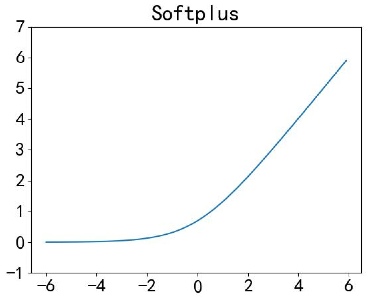
where $z_j^l$ is the value of the j-th node in the i-th layer, $w_{ji}^l$ is the weight between the i-th node in the (l − 1)-th layer and the j-th node in the l-th layer; $b$ represents the connection thresholds. $f$ is an activation function. The softplus function is used as the activation function in this study, as shown below:

$$f\left(x\right)=log\left(1+e^x\right).$$

(2)

The softplus function has the advantages of fast calculation speed and fast convergence speed. The function curve is shown in Figure 1.

3.2. The Convolutional Neural Network

The CNN was originally proposed by LeCun et al. [44] and has been used in many fields, such as image recognition and speech recognition. With the rapid development of deep learning, CNNs have been widely used in recent years. The CNN model generally consists of convolutional layers, pooling layers, and fully connected layers [20].

Each convolutional layer in the CNN model consists of several convolutional units, and the parameters of each convolutional unit are optimized by a back-propagation algorithm. The purpose of the convolution calculation is to extract different features of the inputs. The first convolutional layer may only extract low-level features, and a multi-layer network can iteratively extract more complex characteristics from low-level features.

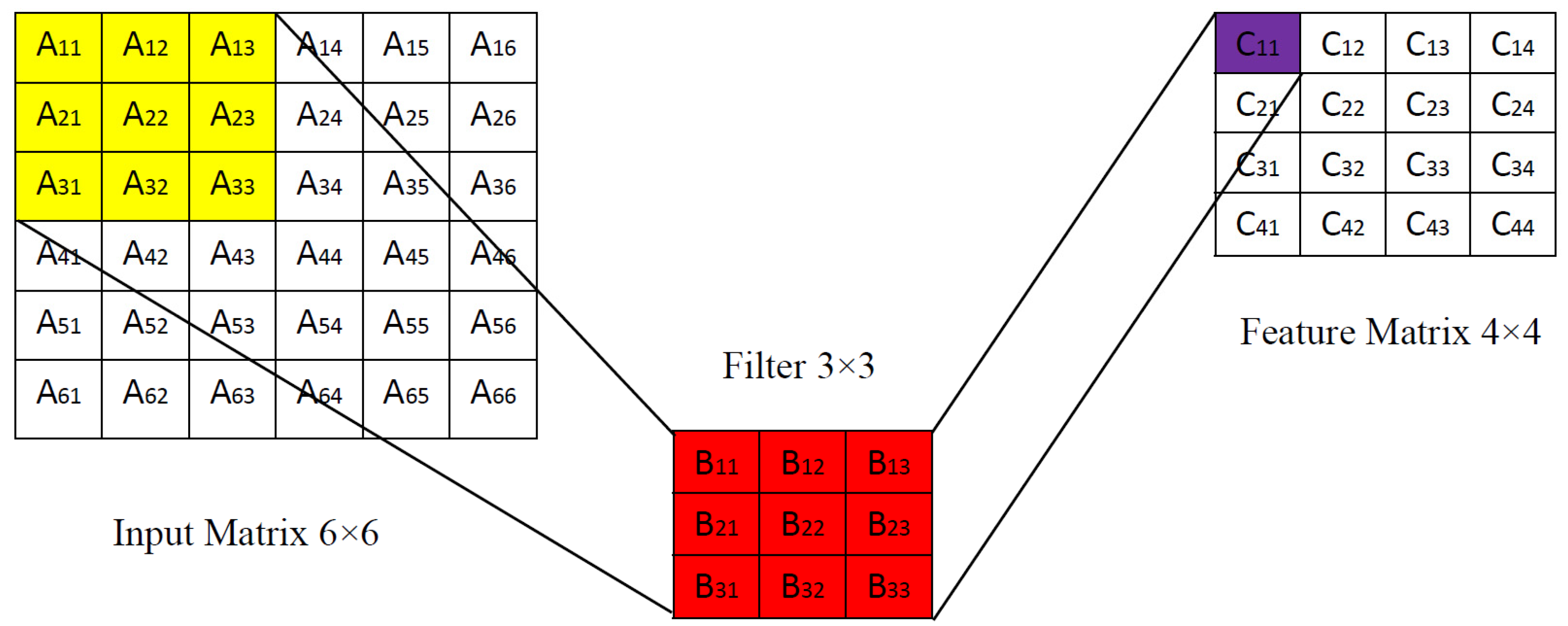
The convolution calculation applies a filter to handle the input data, and the parameters involved include the size of the input matrix $\left(H\times W\right)$, the convolution stride ($S$), the filter size ($FH\times FW$), and the edge padding ($P$). The size of the feature matrix obtained after the calculation is $OH\times OW$:

$$OH=\frac{H-FH+2P}{S}+1,$$

(3)

$$OW=\frac{W-FW+2P}{S}+1.$$

(4)

Taking a single-layer convolution as an example, the calculation process is shown in Figure 2. The input data and the filter have two dimensions, namely height and length. The size of the input matrix is 6 × 6, and the size of the filter is 3 × 3; the stride is 1. The filter performs the convolution calculation at the corresponding position of the input matrix. The calculation of $C_{11}$ is taken as an example, and the formula is shown below:

$$C_{11}={\displaystyle \sum }_{\begin{array}{c}i=1:3\\ j=1:3\end{array}}\left(A_{ij}\times B_{ij}\right).$$

(5)

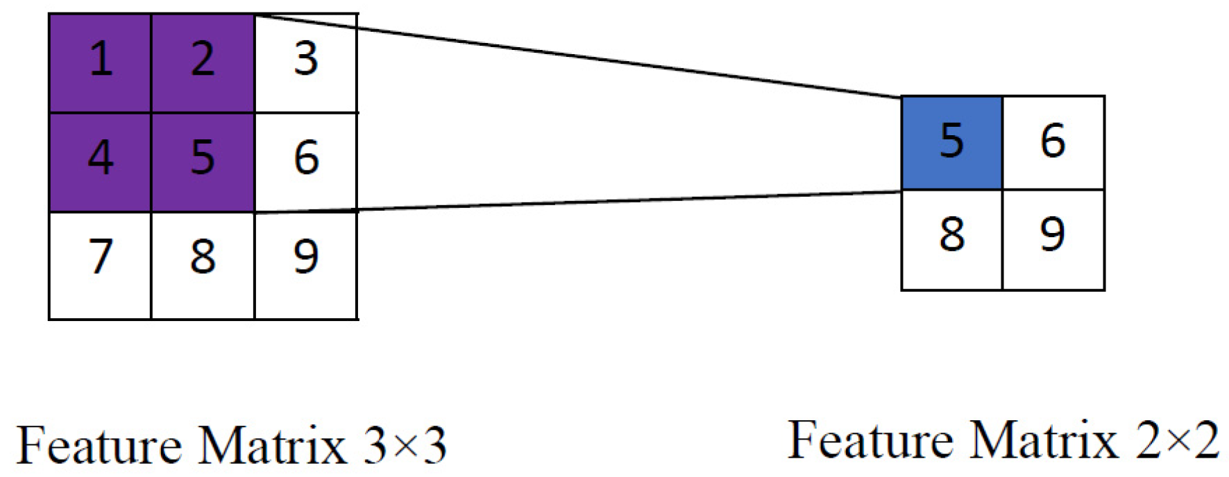
To further reduce the amount of computation, a pooling layer is typically added after the convolutional layer. The pooling layer, also known as the resampling layer, is an important structural layer of CNNs that can reduce the dimensions and summarize the main features. General pooling operations include max-pooling, average-pooling, and adaptive max-pooling. The single-channel max-pooling operation is performed from left to right and from top to bottom, much like the convolution calculation. The max-pooling is performed on a 3 × 3 feature matrix with a pooling stride of 1. The size of the feature matrix after the pooling operation is 2 × 2 (as illustrated in Figure 3). Unlike the convolutional layer, the pooling layer does not learn the relevant parameters; the max-pooling operation only takes the maximum value from the target data. Following the pooling operation, the number of channels of input and output data does not change, and the pooling operation is conducted independently in each channel.

The fully connected layer is usually the last layer of the CNN. Each neuron in the current layer is fully connected to the neuron in the previous layer, and the local information in the convolutional layer or the pooling layer is connected. When the CNN is used to solve regression problems, the fully connected layer uses high-level feature information as input and uses the forecast (fitting) results as output.

3.3. Experimental Design

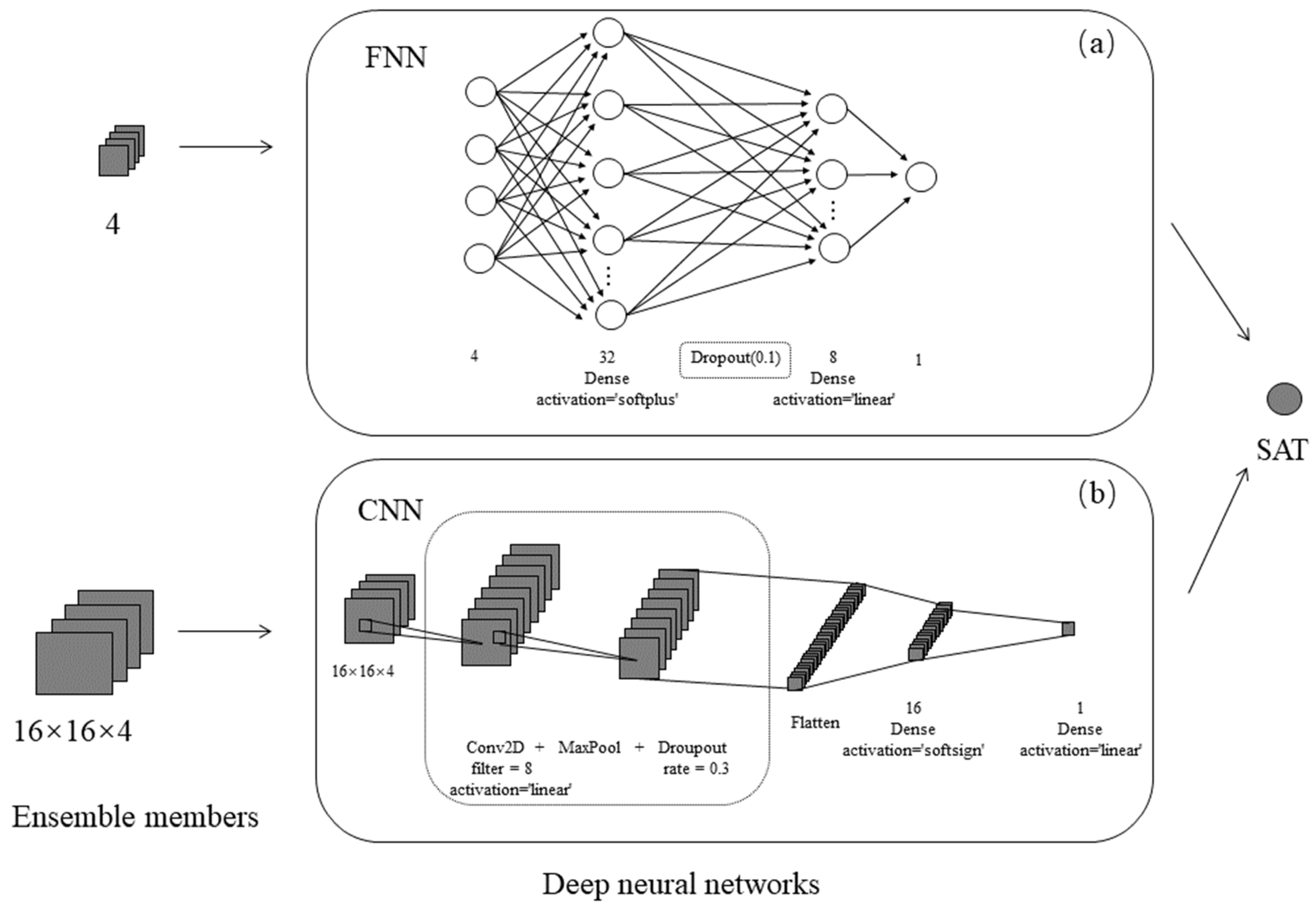
This study uses the CNN and FNN methods for forecasting experiments. The two neural network models were implemented as end-to-end architecture, and their workflows are presented in Figure 4. The daily SAT forecasts over Henan Province and the surrounding areas (109.2°–117.7° E, 30.2°–37.7° N) are extracted and interpolated onto 0.1° × 0.1° grids using a bilinear interpolation method. A relatively small evaluation region (110°–117° E, 31°–37° N) is selected since there is no sufficient data around the boundary for the CNN. Specifically, a 16 × 16 data matrix with 4 features is established for the target points in the evaluation region, and then it is normalized with the Z-score method. The resulting matrix is used as the input data for the CNN model. Upon removing the missing samples, a total of 525 samples are used as the training set, and 131 samples are used for testing.

As mentioned above, the input dataset of the CNN is a 16 × 16 × 4 window of model forecasts. The CNN model used in this study consists of convolutional layers, pooling layers, and fully connected layers (see Figure 4b), and the convolutional layer contains many convolutional blocks [24]. Through a large number of tests, the best results can be obtained by using a linear function in the convolution layer. By setting different parameters in the training process, it can ultimately be determined that the number of filters in the convolutional layer is 8, and the filter size is 2 × 2; the stride is set to 1. Each convolutional block is followed by a max-pooling layer with a 2 × 2 pooling operation and a dropout layer with a rate of 0.3. The test results of two fully connected layers are better than those of multiple or single fully connected layers.

The FNN model consists of two hidden layers with 8 and 32 neurons, with a dropout rate of 0.1. Keras [45], a deep learning API written in Python offers various activation functions, including softmax, ELU, SELU, softplus, softsign, ReLU, and linear. Upon testing all activation functions, we determined that the softplus function in the first hidden layer and linear function in the second hidden layer produced the best experimental results. The glorot_uniform scheme is used to initialize the kernels and biases of the neural nodes.

The final step is the result evaluation. The hit rate within the temperature error of 2 °C (HR2), the MAE and RMSE of the FNN, and the CNN forecast results are calculated. The FNN and CNN models are compared with numerical models to assess their respective strengths and weaknesses.

3.4. Verification Metrics

To quantitatively assess the forecast results of the raw model output and the CNN in Henan Province (110°–116° E, 31°–37° N) from 1 November to 30 December 2020, several metrics are employed: HR2 [25,46], MAE, RMSE, skill score (SS), and pattern correlation coefficient (PCC):

$$\mathrm{HR}2=\frac{1}{n}num(\left|F_i-\left.Y_i\right|\le 2°\mathrm{C})\right.\times 100\%,$$

(6)

$$\mathrm{MAE}=\frac{1}{n}{\displaystyle \sum }_{i=1}^n\left|F_i-Y_i\right|,$$

(7)

$$\mathrm{RMSE}=\sqrt{\frac{1}{n}{\displaystyle \sum }_{i=1}^n{(F_i-Y_i)}^2,}$$

(8)

$$\mathrm{PCC}=\frac{{{\displaystyle \sum }}_{i=1}^n\left(F_i-\overline{F}\right)\left(O_i-\overline{O_i}\right)}{{{\displaystyle \sum }}_{i=1}^n{(F_i-\overline{F})}^2{{\displaystyle \sum }}_{i=1}^n{(O_i-\overline{O_i})}^2},$$

(9)

$$\mathrm{SS}=\frac{A_f-A_r}{A_p-A_r},$$

(10)

where n is the number of stations participating in the forecast, and “num” represents the number of stations that meet the conditions. $F_i$ represents the forecast of the i-th sample, and $Y_i$ represents the corresponding observation value. $A_f$ represents the assessment results of the target model, $A_r$ represents the assessment results of the comparison model, and $A_p$ represents the optimal evaluation results.

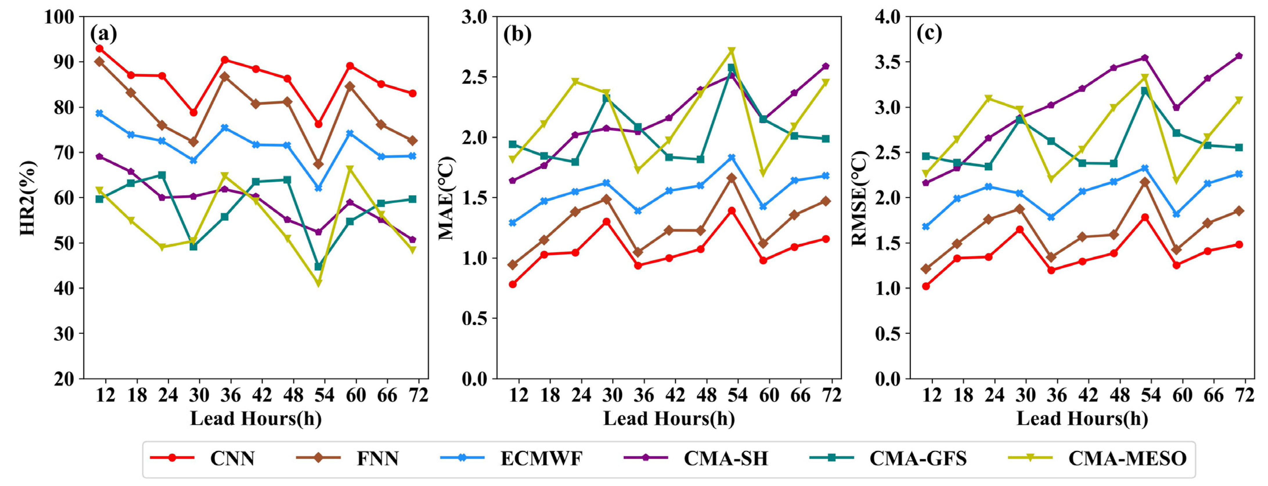
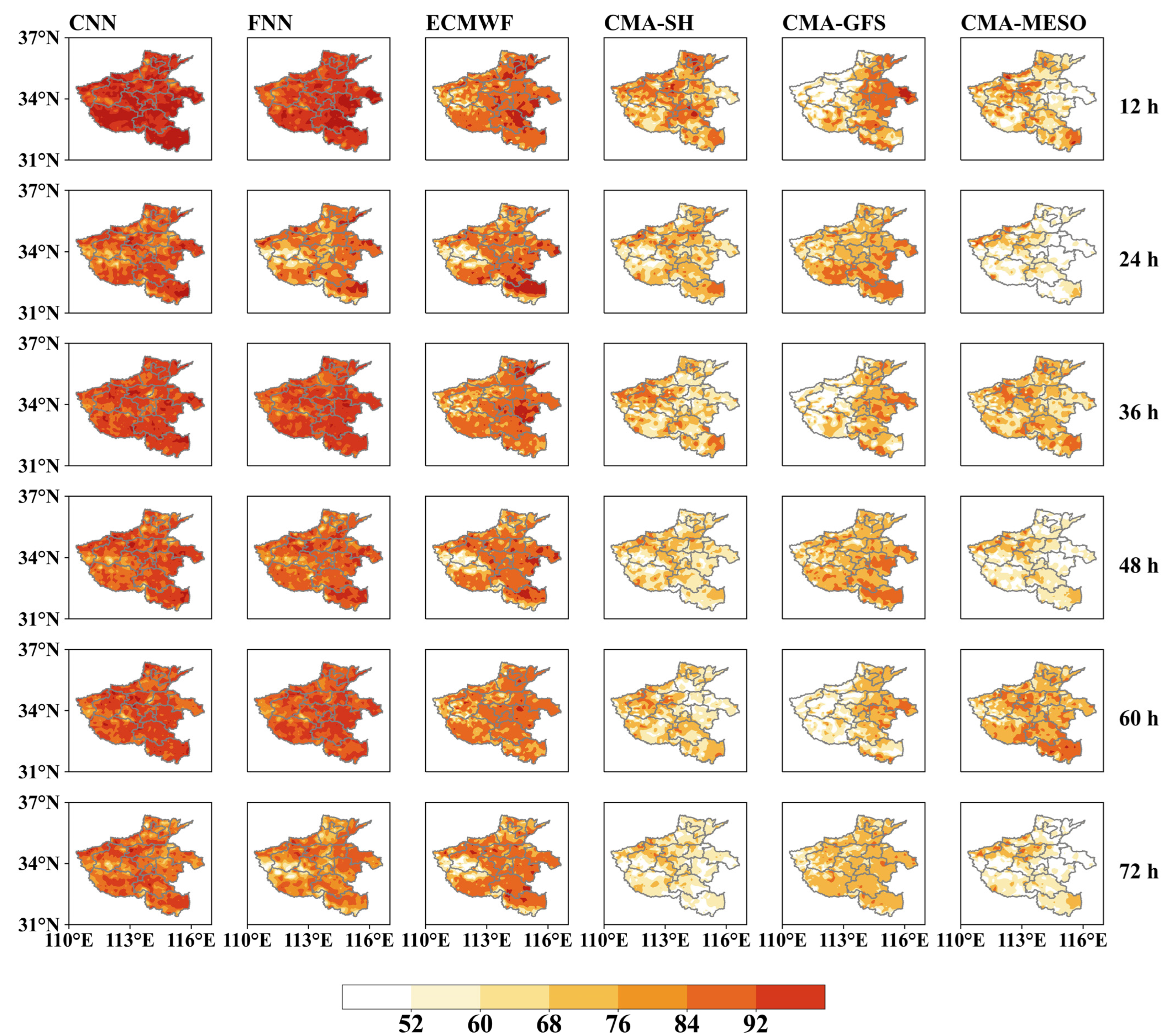
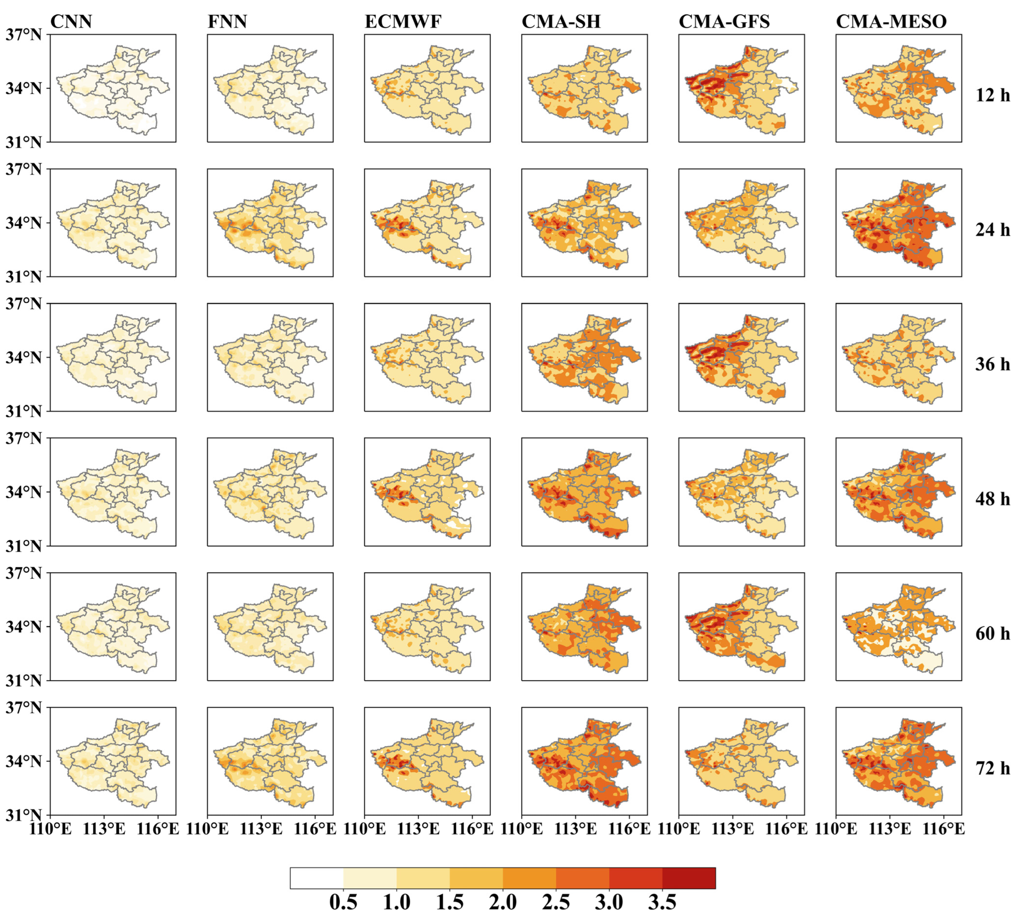
In Section 4, we focus our evaluation and analysis on points within Henan Province. We present the regionally averaged HR2, MAE, and RMSE of the 12–72 h SAT forecasts from the CNN, FNN, ECMWF, CMA-GFS, CMA-SH, and CMA-MESO in Henan Province (see Figure 5). These values are obtained by averaging the errors of each forecast result from the testing period over all grid points in Henan Province with different forecast lead times. 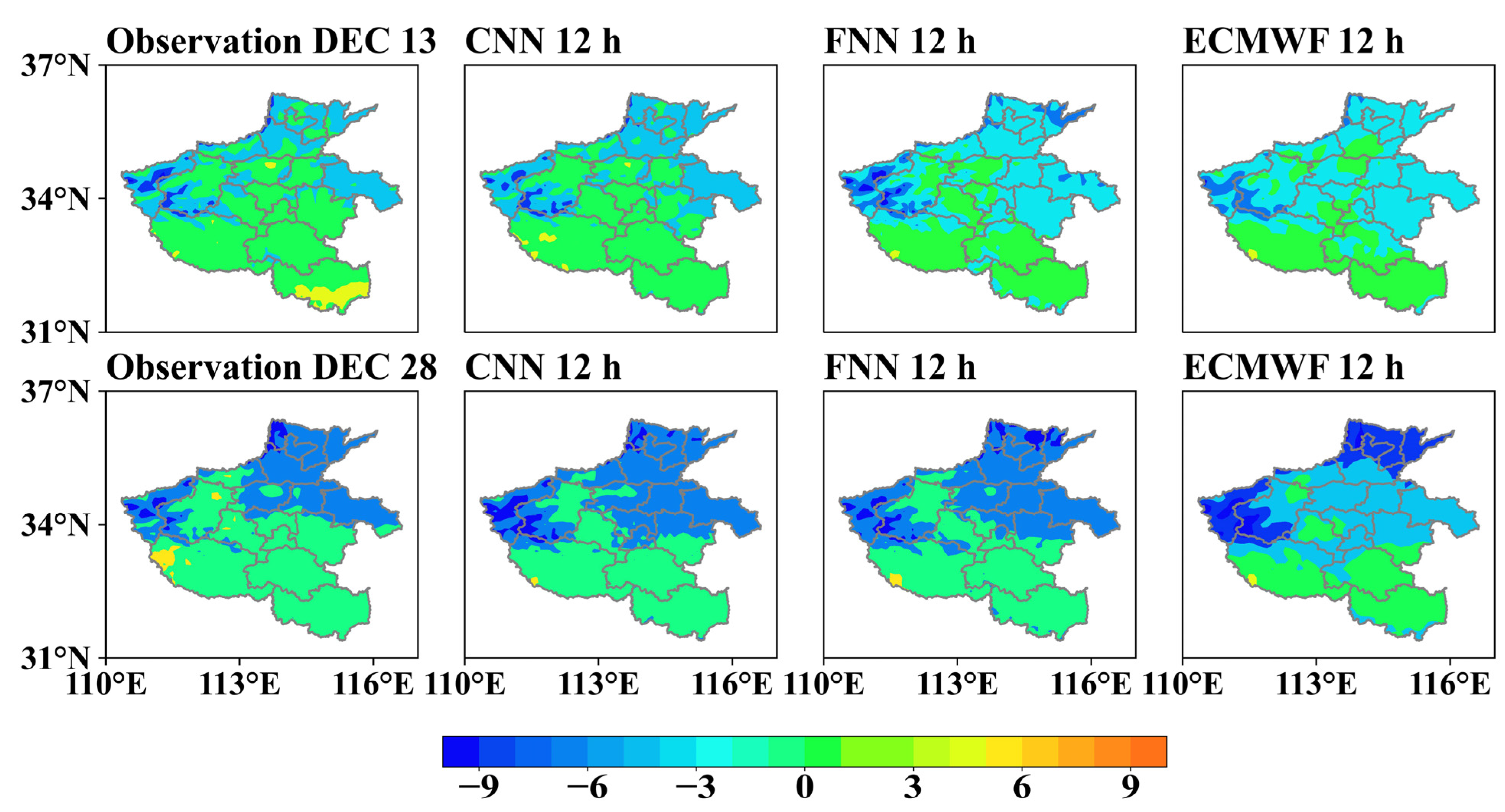The spatial distributions of time-averaged HR2 and MAE with multiple NWP models and post-processing methods are presented in Figure 6 and Figure 7, respectively. The time-averaged HR2 and MAE are calculated by averaging the errors of every forecast result from 1 November to 30 December 2020, with different lead times at each grid point in Henan Province. Similarly, we present the daily area-averaged MAE, which is the average over all grid points per day with different lead times. In addition, we give a figure of the observed and predicted SAT of two cold-wave events, which can visually show model performance. The various graphs included herein show the forecast effects from multiple perspectives.

4. Results

The averaged HR2, RMSE, and MAE of the 12–72 h SAT forecasts for the CNN, FNN, ECMWF, CMA-GFS, CMA-SH, and CMA-MESO in Henan Province from 1 November to 30 December 2020 are presented as follows. A higher HR2 and lower RMSE and MAE demonstrate higher forecast skills, indicating that the ECMWF outperforms the others among the raw NWP models in terms of HR2 (Figure 5). The HR2 values of the ECMWF runs are over 70% at all lead hours, while those of CMA-GFS, CMA-SH, and CMA-MESO are below ~60%. The FNN and CNN also perform better than the ECMWF model, with average improvements of 10% and 15%, respectively. This indicates that the deep neural networks can significantly reduce the SAT forecast errors. The model performance, in terms of the MAE and RMSE, is coincident with that of HR2. The ECMWF serves as the best-performing single model, but the CNN is superior to all of the others. Compared to the ECMWF, the averaged MAE and RMSE values are, respectively, reduced by 0.5 °C and 0.67 °C with the CNN. The results also indicate that the performance of the post-processing methods is highly related to the forecast skills of the raw NWP models, where varying scores are seen with the increased lead times.

The spatial distribution of the forecast skills (as demonstrated by HR2 and MAE) with multiple NWP models and post-processing methods is presented in Figure 6 and Figure 7. The forecasts produced by the CMA models are less accurate over the study region. Clear spatial patterns can be seen in the model performance in terms of HR2 (Figure 6); for example, the CMA-SH performs better in western Henan, while the CMA-GFS achieves higher scores in the eastern part of the province. The ECMWF is still the best single model, especially in the eastern and southern regions, with an HR2 over 75%. However, this indicates that the ECMWF is less capable in western Henan, which is a mountainous region. The varied topography makes it more difficult to provide high-quality SAT forecasts. The deep neural networks further improve the raw NWP model performance, and the CNN is superior to the others. The results demonstrate that both the FNN and CNN significantly increase the HR2 by 85% over the study region. The CNN shows its advantages in the bias correction in the mountainous region (western Henan), which improves the HR2 from around 50% (FNN) to over 80%. This indicates that the CNN is able to capture the spatial features of the atmospheric fields and is therefore more robust in regions with varied topography.

Similar spatial patterns can be observed in the distributions of the MAE (Figure 7). The geographical distributions are obviously different among the models, with different distribution characteristics. The ECMWF serves as the best-performing single model, with an overall MAE around 1.5 °C over the study region. However, poor performance persists in the mountainous region in western Henan. The FNN reduces the forecast error by 1 °C in terms of MAE, but it cannot further improve the SAT forecast in eastern Henan. The CNN outperforms the others with an averaged MAE lower than 1 °C. The spatial distribution of the forecast errors quantitatively demonstrates that the CNN model has the best performance over the study region, especially in the mountainous areas where the raw NWP models and the FNN have much larger forecast errors.

To further analyze the improvement of FNN and CNN in the SAT forecast, the boxplots of the SS of the MAE, HR2, and PCC with lead times of 12–72 h using the CNN and FNN are shown in Figure 8. The interquartile ranges in the boxplots indicate the forecast uncertainty of each method. The plots show that the dispersion degree of the relative deviation of the SAT forecast is small, and the dispersion degree of the CNN is smaller than that of the FNN. The performance of the raw NWP model forecasts varies significantly throughout the study region. The CNN and FNN methods perform competitively in narrowing this disparity, but the CNN approach is best. The SSs of the CNN are higher than the SSs of the FNN.

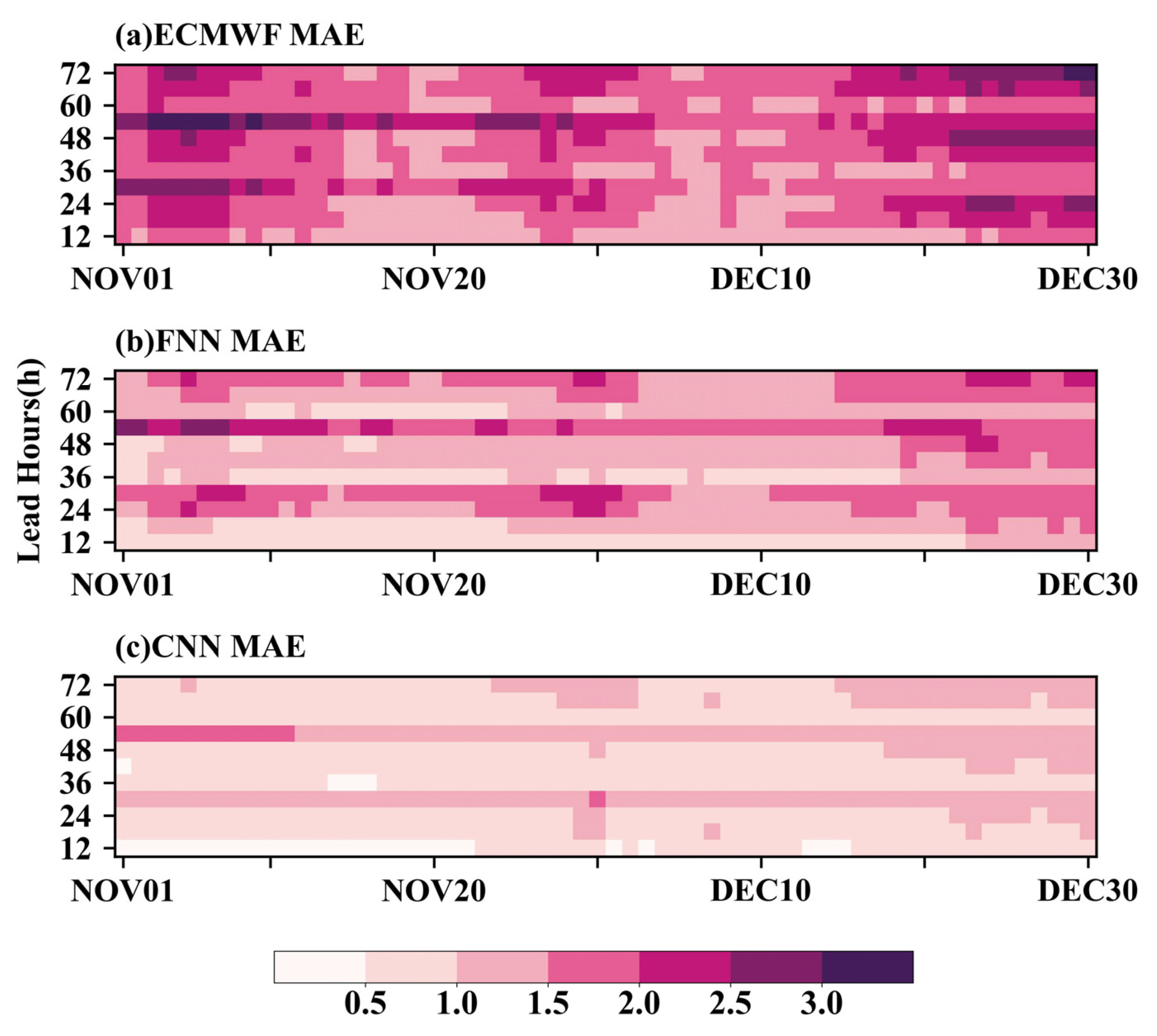
To further assess the FNN and CNN forecasts on hourly bases, the MAEs of the SATs averaged over the study area are displayed in Figure 9 for the ECMWF, FNN, and CNN forecasts, as they approach the target periods with lead times of 12–72 h. The overall MAEs of the ECMWF are the largest, with values between 1 °C and 4 °C. Within the 48 h, the overall MAEs are 1–2.5 °C, with most of them being smaller than 1.5 °C. Beyond the 48-h forecast period, the MAEs increase, with values larger than 3 °C on some days. The FNN and CNN can both calibrate the raw ECMWF forecasts well, with lead times of 12–72 h during all forecast periods. The MAEs of the FNN decrease obviously and do not exceed 2.5 °C, with most values less than 1.5 °C. With the increase in forecast time, the MAEs of the FNN increase slightly. The MAEs of the CNN are the smallest. Most of the MAEs in the forecast period are smaller than 1 °C, with a few around 1.5 °C.

To analyze the SAT forecast errors of the CNN and ECMWF, Figure 10 shows the MAE distributions and scatter plots of the 12-h SAT forecast from the CNN and ECMWF. The proportion of samples with a CNN forecast error smaller than 2 °C is about 95%, and the ratio of samples with an error smaller than 1 °C is about 71%. The distribution of the MAE values for the ECMWF is not as concentrated as that of the CNN. The proportion of samples with an error smaller than 2 °C (1 °C) is about 80% (<50%). Meanwhile, 8% of the forecast results have errors >3 °C. In the error scatter plots, the distance to the diagonal line represents the deviation between the forecast and the observations. The error distribution of the ECMWF is relatively uniform. When the observations are between −10 °C and 5 °C, the proportion of the samples with larger errors and underestimated forecast results is larger, while the forecast value is overestimated when the observation is smaller than −10 °C. Compared with that of the ECMWF, the distribution of the CNN error scatter plot is narrower and more concentrated, which indicates the forecast result is improved. The number of samples with errors smaller than 1 °C increases obviously, while the number with errors larger than 3 °C is remarkably reduced.

According to the historical data, there were two cold-wave events in Henan Province on 13 and 28 December 2020. The temperature on 13 December was 8–12 °C lower than that on 12 December. As shown in Figure 11, the forecast result of the CNN is closer to the observations. For the forecast on 13 December, the CNN shows great advantages in regions with low temperatures, and it is more accurate in northwestern and central Henan. On 28 December 2020, the CNN has a better forecast performance than the ECMWF does in western, northern, and eastern Henan. The range of low temperatures forecasted by the ECMWF is larger than that of the CNN in western and northern Henan, while the situation is the opposite in eastern and central Henan. This result shows that the CNN can depict the abrupt change in the SAT well.

5. Discussion

The CNN’s advantages in the mountainous region indicate that the CNN can capture the spatial features of the atmospheric fields and is therefore more robust in regions with varied topography. Zhu et al. [25] came to a similar conclusion. They compared the SAT forecast performance of U-net with that of three conventional postprocessing methods. Following the four methods, the sequence error in the Altai Mountains, Junggar Basin, and Kunlun Mountains is relatively large, and only U-net significantly reduces the sequence error, which shows that U-net performs better than the other three methods in the above areas. Different neural networks should be trained in different regions given the differences in geographic information (such as altitude, latitude, and longitude) and terrain among different grid points [23]. In future studies, in order to further improve the forecast skill, we can input geographic information from each grid point into the neural network as training data.

Since the CNN can extract features through convolution calculation, it can combine the advantageous features of the four individual models and further improve the forecast skill. Meanwhile, the forecast skill of the CNN within the forecast time period of 12–72 h depends on the forecast skill of the models participating in the multi-model super-ensemble. Therefore, the numerical model selection may affect the quality of the final results. A similar strategy was applied by Zhi et al. [40]. In addition, there are inconsistencies in the raw NWP model performance at different lead times; this problem could be improved by using other methods in a follow-up study.

6. Conclusions

In this study, a CNN- and FNN-based multi-model ensemble of 12–72 h SAT forecasts was run based on ECMWF, CMA-GFS, CMA-SH, and CMA-MESO models. Then, the forecast errors of the CNN, FNN, and four numerical models were evaluated and compared. The main conclusions are as follows.

In general, the forecasts produced by the CMA models were less accurate over the study region, while the ECMWF had the best forecast skill among the four numerical models. The forecast skill of the FNN is better than that of the individual model forecasts in the short-term forecasts. Compared with the ECMWF, which has the best forecast skill among the numerical models, the HR2 of the FNN is increased by 15% on average, and the MAE and RMSE are decreased by 0.27 °C and 0.4 °C on average, respectively. There are geographical differences in the FNN forecast results. The forecast skill is better in eastern and southern Henan, and the improvement is noticeable in western and southwestern Henan.

The CNN has better forecast skills than the FNN does in short-term forecasting. Compared with the ECMWF, the HR2 of the CNN is increased by 22% on average, and the MAE and RMSE are reduced by 0.5 °C and 0.67 °C on average, respectively. The overall MAE of the CNN is smaller than 1 °C, and the percentage of stations with forecast errors within 2 °C is about 95%. The distribution of the CNN error scatter plot is more concentrated, and the dispersion degree of the relative deviation of the CNN is smallest, which means the forecast result is improved. The difference in the geographical distribution of the CNN errors is small, without any apparent high-error areas. The CNN shows its advantages in the bias correction in the mountainous region (western Henan). When forecasting cold waves, the CNN excels in regions with low temperatures and can accurately capture abrupt changes in SAT.