On the Different Quasi-2-Day Wave Behaviors during Sudden Stratospheric Warming Periods

Abstract

The temporal variations in the sudden stratospheric warming (SSW) events in the winter stratosphere always coincide with the quasi-2-day wave (Q2DW) in the summer mesosphere, and the impact of SSW on Q2DW is interesting but still a mystery. Major SSWs occurred in both 2006 and 2009, while the Q2DW activity was quite different. The Second Modern Era-Retrospective Analysis for Research and Applications (MERRA-2) reanalysis dataset was used to comparatively analyze these two major SSW events and elucidate the reasons for the different Q2DW behaviors. We noticed that the summer easterly jet shows a large interannual variability. We conclude that the summer mesospheric Q2DWs are modulated by the winter SSW, whereas the modulation process is also affected by the interannual variability of the summer easterly flow itself. The effects of the SSW on the Q2DWs may differ from year to year due to the variability of the summer easterly flow itself, resulting in different anomalous Q2DW behavior. This conclusion may also be true for the interannual variability of other phenomena during the SSW period.

1. Introduction

Sudden stratospheric warming (SSW) is one of the most drastic dynamical processes occurring at high latitudes, which is more frequently observed from December to February in the northern hemisphere [1,2,3,4]. It is characterized by a sudden increase in the zonal mean temperature and a decrease in easterly winds in the winter stratosphere, both of which are induced by the rapid growth of planetary waves at high latitudes. The easterly winds in the stratosphere are even reversed during a major SSW event, which results in a change in the filtering of gravity waves and enables more easterly gravity waves (GWs) to propagate into the mesosphere. Chandran et al. [5] illustrate the transition of the polar stratopause from being GW-driven phenomena to planetary wave-driven phenomena during SSW events and its subsequent reestablishment and control by GWs. In addition, strong planetary waves in the stratosphere also induce changes in the equatorial regions, which then affect the mean flow in the summer hemisphere.

It is well-accepted that the atmospheric mean flow is essential for the propagation and amplification of planetary waves by modulating their refractive index and the mean flow instability [6]. For example, the Q2DWs are more likely to propagate at middle and low latitudes, where the atmosphere is characterized by a positive refractive index. Similarly, polar planetary waves are more likely to propagate at the mesosphere, as determined by background wind and mean flow instability [7,8,9]. Q2DW amplitudes are much larger in the summer Southern Hemisphere than in the Northern Hemisphere [10,11,12,13]. This is because the mean flow instabilities are associated with the easterly winds in the summer mesosphere, which contribute significantly to the amplification of the Q2DWs. Furthermore, it has been found that Q2DWs with different zonal wavenumbers can be selectively amplified at different times due to the variability of the mean zonal wind and, hence, the Q2DW critical layer.

As a result, the latitudinal and vertical couplings during an SSW event are likely to cause significant variability in the planetary waves. For example, secondary planetary wave signals in the mesosphere and lower thermosphere region of the winter hemisphere immediately followed the occurrence of SSW in January 2012 [14]. The meteor radar chains show that these planetary waves mainly oscillate with zonal wavenumbers 1 and 2 [15]. Qin et al. [16] found that during the sudden Arctic stratospheric warming (SSWs) from 2005 to 2020, eight westward quasi-eight-day wave (Q8DW) events with a zonal wavenumber of 1 (W1) occurred. They found that the reversal (or deceleration) and recovery of the zonal mean flow during SSWs can produce zonally symmetric Q8DW. W1 Q8DW is likely the child wave generated by the nonlinear interaction between a stationary planetary wave with zonal wavenumber 1 and zonally symmetric Q8DW. Teng et al. [17] explore migrating tidal variabilities that occurred during the 2002, 2010, and 2019 Antarctic stratospheric sudden warming events. They suggest that the unexpected decline in the terdiurnal tide with the zonal wavenumber 3 (TW3) may be mainly caused by the nonlinear interaction between the diurnal tide with the zonal wavenumber 1 (DW1) and the semidiurnal tide with the zonal wavenumber 2 (SW2), in which DW1 may play a major role. In the final sudden stratospheric warming in 2016, 2015, and 2005, unusually large westward propagating waves (~10 day) were observed at stratosphere height (about 48 km) and above 55° latitude [18]. The results show that both the occurrence of SSW and the seasonal timing of SSW are important factors for the transient variability of Q10DW. Wang et al. [19] combined observations from microwave limb sounder with the sounding of the atmosphere using broadband emission radiometry and meteor radar wind measurements from Antarctica. This provides a comprehensive view of Q10DW wave activity in the Southern Hemisphere during the 2019 unusual sudden stratospheric warming. Their analysis showed that Q10DW of various wavenumbers could be excited by nonlinear wave–wave interactions, which also include stationary planetary waves with s = 1 and s = 2. Rhodes et al. [20] use the National Center for Atmospheric Research’s Whole Atmosphere Community Climate Model with specified dynamics (WACCM+SD) to study the eastward-propagating planetary waves (EPWs) in January 2009 at northern latitudes during the 2009 major SSW. They found that EPWs can significantly influence mesospheric wind structure and play a key role in the nature and timing of SSW events. In particular, EPWs help to reduce pre-existing wind shear, thereby stabilizing the polar vortex. Sato et al. [21] suggested that the maximum potential vorticity in the winter and summer mesospheres is caused by parametric GW forcing, which was investigated using simulations data from a whole-atmosphere model.

As one of the most robust periodical oscillations in the MLT region, the temporal variations of the Q2DW always coincide with the SSW. The enhancement of Q2DW activities has also been identified both in the equatorial region and at low latitudes during the SSW periods [22,23,24]. It is found that the strong planetary waves (SPWs) during an SSW event may nonlinearly interact with Q2DWs, which generates new Q2DWs with different zonal wavenumbers [25,26,27]. The Navy Operational Global Atmospheric Prediction System-Advanced Level Physics High Altitude (NOGAPS-ALPHA) reanalysis dataset has been successfully utilized for the study of both SSW and Q2DW [28,29,30,31,32]. However, due to the complex interannual variabilities of both the SSWs and the Q2DWs, the impact of the SSW on Q2DW is still not understood.

We note that during the major SSW period of 2006, the Q2DW exhibits abnormally strong oscillations with zonal wavenumber 2 and 3 [33], which is attributed to both the nonlinear interaction with SPW and the strong summer easterly jet [26]. Nevertheless, though the 2009 major SSW is nearly the strongest SSW event of the past two decades, the W3 Q2DW is nearly the weakest of the past decade. Meanwhile, the W4 Q2DW in January 2009 is abnormally strong compared to that of other austral summer periods. In this paper, we use the Thermosphere, Ionosphere, Mesosphere, Energetics, and Dynamics (TIMED) satellite datasets to investigate the W1, W2, W3, and W4 westward propagating waves in the mesosphere during 2006 and 2009; the Second Modern-Era Retrospective Analysis for Research and Applications (MERRA-2) reanalysis datasets are analyzed in detail. We would like to determine what caused the different Q2DW behaviors during these two major SSW periods. The dataset and the analysis are described in Section 2, and the analysis results in 2006 and 2009 are comparatively presented in Section 3. Finally, our new findings are concluded in Section 4.

2. Data and Analysis

To perform diagnostic analysis on the dynamic process of SSW and Q2DW, we need both synoptic temperature and wind datasets, especially for the stratosphere and mesosphere. The Sounding of the Atmosphere using Broadband Emission Radiometry (SABER) datasets from the TIMED satellite are optimal for studying the variability of Q2DWs, as they completely cover the vertical region of the mid-atmosphere where the waves are strongest. Their resolution is ~4° for latitude, with a vertical resolution of ~4 km in the stratosphere and mesosphere. The SABER temperature data focus on a region of approximately 20 to 100 km. The SABER sampling has two positions of ~50° S–80° N and ~80° S–50° N, changing every ~60 days. The least squares fitting method was used to fit the observed SABER temperature data, and the W1, W2, W3, W4 Q2DW were extracted. In our analysis, we used a 6-day temporal window to perform a 2-day step analysis for waves in the period from 36 h to 72 h. The period and wavenumber corresponding to the largest amplitude in the spectrum are taken as the wavenumber and period of the spatial structure analysis window. The vertical and latitude boxes are 2 km and 5°, respectively. The Q2DW events were extracted from the temperature data measured by SABER in 2006 and 2009; these were observed at ~30–40° S and ~67–73 km for W4, and ~30–40° S and ~77–83 km for W3; ~20–30° S and ~87–93 km for W2; ~10–20° S and ~77–83 km for W1.

The Second Modern-Era Retrospective Analysis for Research and Applications (MERRA-2) reanalysis data [34] are used to provide more comprehensive atmospheric data for studying the structural behaviors of different Q2DWs during the 2006 and 2009 SSW periods. The temporal resolution (~1 h), vertical resolution (~2–3 km), and spatial resolution (~0.5 × 0.625) of the MERRA-2 data were fixed (Note: 5/8° longitude, 1/2° latitude). The long-term MERRA-2 data in 2006 and 2009 were used to diagnose the contribution of SSW with different periods to W1, W2, W3, and W4 during the summer and to analyze background winds, instabilities, and source activity.

A two-dimensional least squares fitting method is adopted to extract planetary wave signals from the dataset, which are then utilized for diagnostic analysis.

$$y=Acos\left[2\pi \left(\sigma ·t+s·\lambda \right)\right]+Bsin\left[2\pi \left(\sigma ·t+s·\lambda \right)\right]+C$$

(1)

The amplitude of a planetary wave can be defined as $R=\sqrt{A^2+B^2}$. The fitted parameter variables are A, B, and C in Formula (1), respectively. The planetary wave frequency and zonal wavenumber correspond to $\sigma$ and $s$, respectively. The UT time and longitude of the satellite sample are $t$ and $\lambda ,$ respectively. C denotes mean temperature.

In the spatial structure of the atmosphere, barotropic/baroclinic instability may occur in regions with negative latitudinal gradients and quasigeostrophic potential vorticity ($\overline{q_{\phi }}$).

$$\overline{q_{\phi }}=2\Omega \cos \phi -{\left(\frac{{\left(\overline{u}cos\phi \right)}_{\phi }}{acos\phi }\right)}_{\phi }-\frac{a}{\rho }{\left(\frac{f^2}{N^2}\rho \overline{u_z}\right)}_z$$

(2)

In Equation (2), the Coriolis parameter, Earth radius, and background air density correspond to $f$, $a$, and $\rho$, respectively; $\Omega$ is the angular speed of the Earth’s rotation; $\overline{u}$ is the zonal mean zonal wind; $\phi$ is the latitude; N is the buoyancy frequency; subscripts $z$ and $\phi$ are the vertical and latitudinal gradients.

3. Anomalous Q2DW Behaviors during the 2006 and 2009 Major SSW Periods

Figure 1a,c shows the mean zonal wind at 60° N during the 2006 and 2009 SSW periods, respectively. Figure 1b,d shows the zonal mean temperature at 70° N and 10 hPa during the 2006 and 2009 SSW periods, respectively. The zonal wind reverses dramatically during both years, indicating the occurrence of major SSWs. During the 2006 Arctic SSW event, it can be seen that the zonal mean zonal wind at 60° N began to reverse in the upper mesosphere on the 7th day. Meanwhile, the temperature at 70° N and 10 hPa also started to increase on this day. Subsequently, the zonal wind direction in the lower layers also began to reverse, and the temperature continued to increase. On the 24th day, the temperature reached its maximum during this SSW and the zonal wind started to recover. Thus, the 7th is defined as the onset day of the 2006 Arctic SSW and the 24th represents the day when the temperature reached its maximum. For the 2009 Arctic SSW event, the moment at which the zonal wind began to reverse and the temperature began to increase occurred on the 17th day. On the 24th day, the temperature reached its maximum during the 2009 Arctic SSW event. Thus, the 17th is defined as the onset day of the 2009 Arctic SSW and the 24th represents the day when the temperature reached its maximum. The vertical black and red lines indicate the starting of the sudden stratospheric warming and the warming peak of the sudden stratospheric warming. In 2006, the zonal mean temperature at 70° N and 10 hPa increases from ~215 K on day 7 to ~240 K on day 24; the zonal mean wind shifted from ~45 m/s on day 7 to ~−50 m/s on day 24, lasting 17 days. The zonal mean temperature increases more sharply in 2009 from ~200 K on day 17 to ~255 K on day 24; the zonal mean wind shifted from ~85 m/s on day 17 to ~−45 m/s on day 24, which lasted for 7 days. The range of SSW during 2006 and 2009 was approximately ~7–24 days and ~17–24 days, respectively. We found that the zonal mean temperature change in 2009 SSW was more rapid than that in 2006, but the temperature change in 2006 first increased, then slightly decreased and then increased. The SSW in 2009 is the strongest event in the past two decades. We will then study the Q2DW behaviors during these two major SSW periods.

Figure 2 shows the peaking dates, amplitudes, and periods of the W1, W2, W3, and W4 Q2DW modes during both 2006 and 2009. The SABER observed altitudes of W1, W2, W3, and W4 were ~80 km, ~90 km, ~80 km, and ~70 km, and the latitudes with the largest amplitudes were ~20° S, ~20° S, ~40° S, and ~40° S, as shown in Figure 2. According to the maximum amplitude of the spectrum, the period and wavenumber of the event are obtained, and then the temporal–latitude structure is analyzed by fixing the period and wavenumber. The fixed wave periods of W1, W2, W3, and W4 were ~43 h, ~43 h, ~44 h, and ~67 h during 2006 and ~53 h, ~42 h, ~46 h, and ~65 h in 2009, respectively. During 2006, the maximum amplitude of W1, W2, W3, and W4 reached ~5 K on days 6–12, ~8 K on days 24–30, ~17 K on days 16–22, and ~3 K on days 20–26, respectively. In 2009, it was ~5 K on days 14–20, ~5 K on days 22–28, ~6 K on days 22–28, and ~5 K on days 44–50. We found that W2 and W3 had temperature amplitudes of 20–30° and 30–40° in the Northern Hemisphere in 2006 and 2009. In 2006 and 2009, W2 and W3 were ~7 K in the Northern Hemisphere. It can be found that there is an unusually strong W2 Q2DW in 2006 and 2009. In addition, in 2006, there was an unusually strong W3 oscillation, but W4 was very weak, and in 2009, there was a W3 oscillation weak, but there was a distinct W4.

The spectral structure of temperature is shown in Figure 3. Figure 3a,e shows the maximum W1 amplitudes at ~80 km and ~15° S of SABER temperature at 16–22 and 26–32 days in 2006 and 2009, respectively. A westward wavenumber 1 signal is found at ~43 h (~3 K) and ~44 h (~3 K), respectively. In addition, Figure 3a also contains the strongest signal with a westward wavenumber of 3 (~8 K, ~43 h). Figure 3b,d shows the maximum amplitude of W2 at ~90 km and ~25° S on 22–28 and 22–28 days between 2006 and 2009, respectively. A westward wavenumber 2 signal is fixed at ~44 h (~6 K) and ~42 h (~6 K), respectively. In addition, there is also the strongest signal with an eastward wavenumber of −2 (~7 K, ~49 h) in Figure 3b and a westward wavenumber of 3 (~6 K, ~47 h) in Figure 3f. Figure 3c,g shows the maximum W3 at ~80 km and ~35° S on days 16–22 and 20–26 during 2006 and 2009, respectively. A westward wavenumber 3 signal is fixed at ~44 h (~13 K) and ~46 h (~4 K), respectively. In addition, Figure 3c also contains the strongest signal with an eastward wavenumber of −2 (~11 K, 51 h). Figure 3d,h shows the maximum W4 at ~70 km and ~35° S on 44–50 days and 44–50 days during 2006 and 2009, respectively. A westward wavenumber of 4 is fixed at ~67 h (~2 K) and ~65 h (~4 K), respectively.

The temperature spatial structures of W1, W2, W3, and W4 in 2006 and 2009 are shown in the panels of Figure 4, respectively. In the temperature spatial structure of 2006 shown in Figure 4a–d, W1 reaches its maximum amplitude at ~10–20° S and ~82 km, which is ~3 K with fixed ~43 h on days 16–22. The temperature amplitude of W2 is ~8 K with fixed ~44 h on days 22–28 at ~20–30° S and ~88 km. The temperature amplitude of W3 is ~17 K with fixed ~44 h on days 16–22 at ~30–40° S and ~82 km, and there is a peak amplitude of ~11 K at ~70 km. The maximum amplitude of W4 is ~2 K with a fixed ~67 h on days 44–50 in the ~30–40° S and 70 km. In the temperature spatial structure of 2009 shown in Figure 4e–h, W1 reaches its maximum amplitude at ~10–20° S and ~90 km, which is ~5 K with fixed ~43 h on days 26–32. The temperature amplitude of W2 is ~7 K with fixed ~42 h on days 22–28 at ~20–30° S and ~90 km. The temperature amplitude of W3 is ~6 K with fixed ~46 h on days 20–26 at ~30–40° S and ~82 km, and there is a peak amplitude of ~6 K at ~60 km. The temperature amplitude of W4 is ~6 K with fixed ~65 h on days 44–50 at ~30–40° S and ~70 km, and there is a peak of ~5 K at ~80 km. The amplitude of the temperature spatial structure of W2 and W3 in 2006 SSW was stronger than that in the 2009 SSW. However, the temperature amplitude of W4 in the 2006 SSW was weaker than in the 2009 SSW.

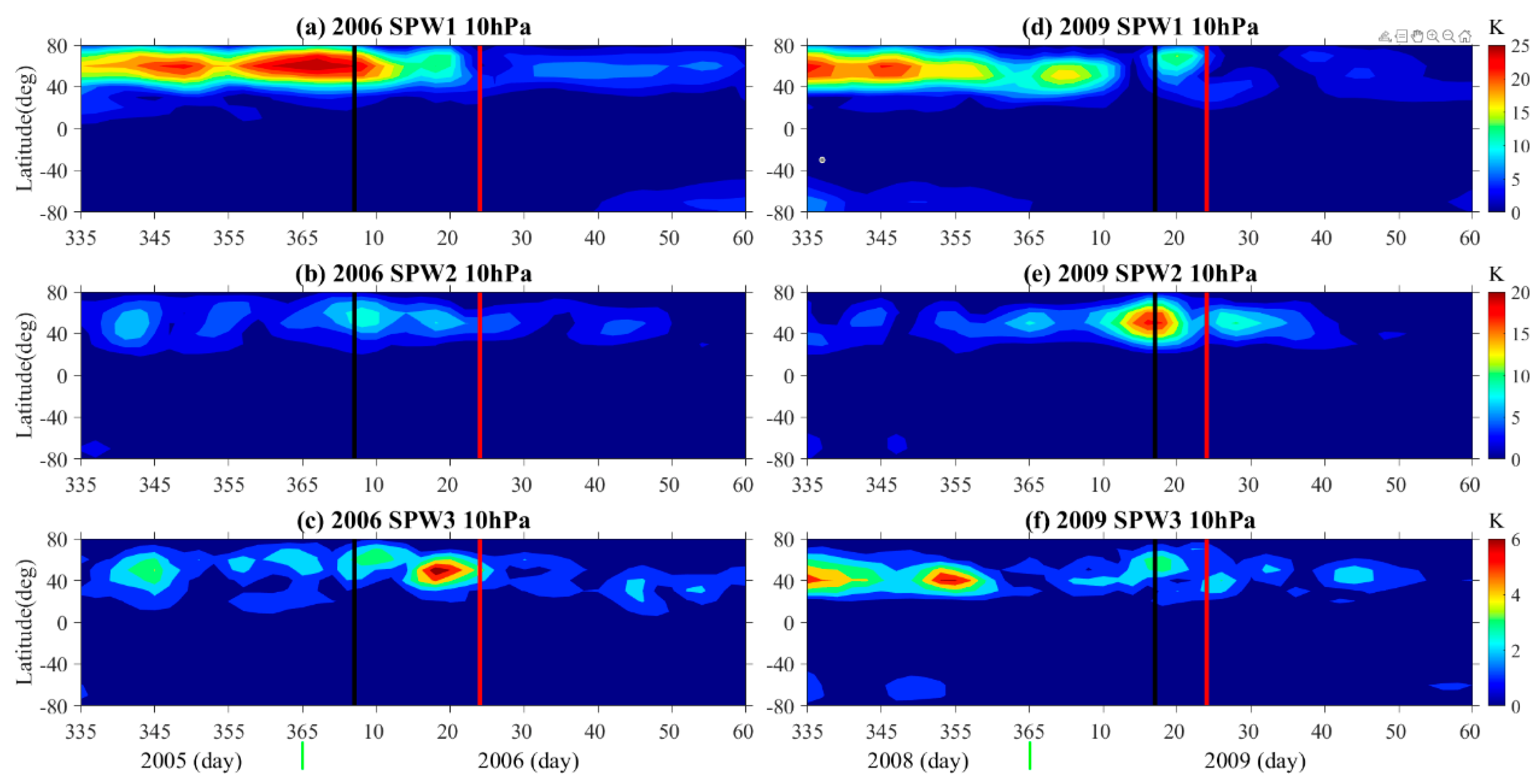
The temporal variations of the stationary planetary wave with wavenumber 1 (SPW1), 2 (SPW2), and 3 (SPW3) at 10 hPa are shown in Figure 5. The vertical black and red lines indicate the starting of the sudden stratospheric warming and the warming peak of the sudden stratospheric warming. Figure 5a shows that SPW1 gradually decreases at the beginning of the 2006 SSW and then reaches an amplitude of ~15 K; however, there is no intensity-to-weakness process in SPW1 in the 2009 SSW. The process of change of SPW2 in 2006 and 2009 is essentially similar, but the amplitude of SSW in 2009 is significantly stronger than that of 2006 (~10 K), reaching ~20 K, as shown in Figure 5b. The performance of SPW3 for the 2006 SSW (~7 K) is significantly stronger than that for the 2009 SSW (~3 K) (Figure 5c). It is found that SPW1 is stronger at the beginning of the SSW in 2006 than in 2009, while SPW2 is the opposite. In 2009, it was nearly two times stronger than in 2006, and SPW3 showed little difference between 2006 and 2009.

Q2DW is a planetary wave propagating and amplifying from the lower atmosphere to the upper atmosphere. Therefore, source activity is the potential factor for the different behavior of Q2DW. Figure 6 shows the geopotential height (GPH) amplitudes derived from the MERRA2 data at ~10 hPa for the W1, W2, W3, and W4 events during the 2006 and 2009 periods. Figure 6a–d shows the 2006 GPH for W1, W2, W3, and W4. The GPH amplitude of W1 during SSW reaches ~80 m. W2 is ~25 m; W3 is ~22 m; W4 is ~12 m. Similarly, the GPH of W1, W2, W3, and W4 in 2009 was shown in Figure 6e–h, and the GPH amplitude of W1 was ~40 m during SSW. W2 is ~70 m; W3 is ~25 m; W4 is ~20 m. It is clearly found that the source activity in W1 is nearly two times stronger in 2006 than in 2009, while the opposite is true for W2, which is nearly three times stronger in 2009. The W3 source activity was similar in 2006 and 2009, but the W4 source activity in 2009 was also nearly two times stronger than in 2006.

Figure 7a–h shows the diagnostic analysis of W1, W2, W3, and W4 events in 2006 and 2009, respectively. According to the events shown in Figure 4, their occurrence date can be determined, and the propagation and amplification of planetary waves with different zonal wavenumbers can be analyzed through the MERRA2 data. In the diagnostic analysis, the shaded regions are instability, and the red line is the zero-wind layer. The solid line is the westerly wind and the dotted line is the easterly wind. W1, W2, W3, and W4 are more conducive to propagation and amplification in the Southern Hemisphere summer due to mean flow instability between 40 and 60° S and 70 to 80 km and appropriate background winds. As shown in Figure 7a–d, the background winds in W1 and W3 are stronger than those in W2 and W4, with W4 being the weakest. In addition, W1, W2, and W3 have similar mean flow instabilities, while W4 is the weakest. The background wind intensity is similar for W1, W2, and W3, but weaker for W4. In addition, the mean flow instabilities of W1, W2, W3, and W4 are similar, as shown in Figure 7e–h. It is worth noting that during the 2009 SSW, easterly winds in the Northern Hemisphere, crossing the atmosphere at altitudes of 20–30 km, a phenomenon not observed during the 2006 SSW. We believe that Q2DWs behavior is influenced by the interaction of the summer easterly jet in the Southern Hemisphere. The adaptability of different zonal wave numbers to the background environment is different, resulting in the selective amplification and propagation of Q2DWs with different zonal wave numbers by the average zonal wind. It can be seen that SSW has an impact on Q2DWs behavior.

Temporal and altitude variations of the zonal mean zonal wind at 40° S in (Figure 8a) 2006 and (Figure 8b) 2009. It can be seen that from the 1 days to the 60 days of 2006 (40° S), the background wind was mainly easterly, reaching ~−85 m/s on 10 days. At the same time, the background wind was mainly easterly, with ~−80 m/s on 20 days from early 2009 (40° S). It can be seen that the easterly winds in the summer of 2006 were stronger than those in the 2009 SSW period. In other words, different background zonal winds may select different zonal wavenumbers to amplify planetary waves. We believe that the fluctuations of different zonal wavenumbers have different responses to background zonal wind, and the mean zonal wind amplifies and propagates the zonal wavenumbers selected to adapt, thus resulting in the selective propagation of the mean zonal wind.

4. Conclusions and Summary

In this paper, we studied both the different Q2DW behaviors during the major SSW periods of 2006 and 2009 with TIMED/SABER temperature observation and MERRA-2 reanalysis, including their temporal variations, wave periods, and wave amplitudes. It can be seen that W1 had a longer wave period in 2009 than in 2006, W2 had a stronger strongest amplitude in 2006 than in 2009, W3 had a largest maximum in amplitude in 2006 than in 2009, and W4 had a weak performance in 2006. However, there was a strong fluctuation in 44–50 days of 2009. According to previous statistical analysis, the W3 maximizes in late January, which is consistent with the results in 2006 and 2009 presented in this paper. Nevertheless, the behaviors of W2 and W4 during these two years are contradictory to their climatological features [35], which is that the W2 mode is the first one to be amplified and the W4 mode is the last one. Their anomalous temporal behaviors strongly suggest the occurrence of nonlinear interactions between Q2DWs and SPWs during the SSW periods with strong winter planetary waves [25,26], which generates Q2DWs with new zonal wavenumbers.

The nonlinear interaction between the W3 and the SPW1 always results in the generation of W2 and W4 Q2DWs. Nevertheless, we found that W2 was amplified during SSW 2006; W4 was not. In addition, W4 was amplified during SSW 2009, W2 was not. The study [36] has shown that the Q2DWs with different zonal wavenumbers are selectively amplified by the zonal mean zonal wind. We also note that the W3 oscillations are very strong in 2006 but extremely weak in 2009. This is also related to the weaker summer easterly jet, which provides weaker mean flow instabilities and Q2DW forcing. The enhanced residual circulation in the stratosphere, induced by strong planetary waves during the major SSW period provides additional Q2DW forcing in both tropical and extratropical regions, which results in strong W3 activities in January 2006 [32]. It has been found that the feedback between gravity wave breaking and the mean flow in the mesosphere also contributes to the interhemispheric couplings during the SSW period [36,37]. We would like to investigate whether or not the weak summer easterly in January 2009 is due to the weaker interhemispheric coupling during the 2009 major SSW. Usually, W3 Q2DW dominates the Q2DW behavior during the austral summer period [38], while Limpasuvan and Wu [33] observed the line-of-sight wind through Aura/MLS during the January 2006 SSW, and a strong W2 Q2DW signal was found. They believe that the coexistence of W3 and W2 Q2DW modes is probably related to the strong summer easterly jet. Gu et al. [26] clearly confirm9 that the summer easterly jet in January 2006 is indeed stronger than that in January 2005. The phase speed of W2 Q2DW is larger than that of W3 Q2DW. Therefore, a stronger summer easterly jet is required to maintain the critical layer of W2 Q2DW, which is crucial for the amplification of W2 Q2DW.

We can see that the interhemispheric coupling during the SSW period of 2009 is even stronger than that of 2006, and thus is not responsible for the weak summer easterly. The temporal variations of the zonal mean zonal wind at 40° S are shown in Figure 8a,b, which show that the summer easterly in the stratosphere and mesosphere are weak from the beginning of the year, which is most likely due to the interannual variations of the mean flow itself.

The conclusions of this paper are shown below: 1. This is the first comparative study on the Q2DW during the 2006 and 2009 major SSW periods. The reversal (warming) of the mean zonal wind (temperature) in 2006 was less drastic than in 2009, indicating that the SSW in 2009 was faster and stronger. 2. Both anomalous Q2DW behaviors are identified in these two major SSW events but with different characteristics. The summer mesospheric Q2DWs are modulated by the winter SSW, whereas the modulation process is also affected by the interannual variability of the summer easterly flow itself. 3. The different features of these two major SSW events result in different anomalous Q2DW behaviors. The different characteristics of the two SSW events and the different easterly jets in summer may lead to different Q2DWs behavior. 4. The consequence of the SSW impact on Q2DW is strongly dependent on the summer easterly itself.

We suggest that the SSWs do have a significant impact on the Q2DWs in both 2006 and 2009 through both nonlinear interactions and interhemispheric couplings; however, the final patterns of expression are different. There is an anomalously strong W2 Q2DW during the 2006 major SSW period with also an extraordinarily robust W3 oscillation, while the W4 wave mode is unusually strong in 2009 but with an extremely weak W3 Q2DW. This is related to the stronger easterly flow in 2006 with respect to 2009, which determines the selective amplification of Q2DWs. Thus, the consequences of the SSW impact on Q2DWs may be different from year to year due to the variabilities of the summer easterly itself, which result in different anomalous Q2DW behaviors. This conclusion may also apply to the interannual variability of another phenomenon during SSW periods.