Feasibility of Downscaling Satellite-Based Precipitation Estimates Using Soil Moisture Derived from Land Surface Temperature

Abstract

For many areas, satellite-based precipitation products or reanalysis model data represent the only available precipitation information. Unfortunately, the resolution of these datasets is generally too coarse for many applications. A very promising downscaling approach is to use soil moisture due to its clear physical connection to precipitation. We investigate the feasibility of using soil moisture derived from land surface temperature in this context. These data are more widely available in the required resolution compared to other soil moisture data. Rain gauge-adjusted radar data from Namoi serves as a spatial reference dataset for two objectives: to identify the most suitable globally available precipitation dataset and to explore the precipitation information contained in the soil moisture data. The results show that these soil moisture data cannot be used to downscale satellite-based precipitation data to a high resolution because of cloud cover interference. Therefore, the Integrated Multi-satellitE Retrievals for GPM (IMERG) late data represents the best precipitation dataset for many areas in Australia that require timely precipitation information, according to this study.

1. Introduction

The objective of the paper is to find the best precipitation data with the shortest possible timestep that is available in near-real-time for the whole of Australia.

In general, and in particular, in Australia, precipitation measurement information availability is very heterogeneous. In this study, as part of the WaterSENSE project, remote sensing data are explored to provide more uniform information.

The goal of WaterSENSE is to develop a modular, operational, water-monitoring system built on Copernicus EO (Earth Observation) data. This will provide water managers and the agricultural sector with a toolbox of reliable and actionable information on water availability and water use anywhere in the world in support of sustainable water management and transparency across the entire water value chain.

As part of this, we designed a modular approach in which the best available precipitation information is used at every location. Where available, quality-controlled and gauge-adjusted radar data are used in accordance with Einfalt and Frerk [1] and Willems and Einfalt [2]. This was implemented in our pilot region in Namoi, Australia. In addition to providing local stakeholders with high-quality precipitation information, this setup is also used as a testbed for other spatial precipitation datasets.

Where radar and rain gauge data are not available, satellite-based precipitation data presents a viable alternative. However, despite considerable advances in this field, as identified by Pellarin et al. [3] and Brocca et al. [4], these data still suffer from inaccuracies and a spatial resolution that is too low for many applications (He et al. [5] and Chen et al. [6]).

Therefore, different approaches were successfully explored by different authors on how to use soil moisture inferred from EO to derive or improve existing precipitation data. For example, in 2008, Pellarin et al. [7] used soil moisture indicated by the polarization ratio inferred from passive microwave measurements at 6.9 GHz from the Advanced Microwave Scanning Radiometer-EOS (AMSR-E) (Jackson et al. [8]) sensor to eliminate false rainfall events from a satellite-based precipitation estimate. Moreover, in 2009, Crow et al. [9] used AMSR-E brightness temperature to correct satellite-based precipitation with the help of a simple Antecedent Precipitation Index (API). Later, Pellarin et al. [3] used a modification of the same approach, named PrISM, in combination with SMOS (Soil Moisture and Ocean Salinity) (Kerr et al. [10]) soil moisture estimates to correct satellite precipitation. Their results compared favorably against uncorrected existing satellite-based precipitation with a short latency (up to a few days) and were comparable with post-processed versions of satellite precipitation with a much longer latency. The comparison was performed on a daily time scale and a 0.25° spatial resolution. In 2013, Brocca et al. [11] developed the method of soil moisture to rain (SM2RAIN) to derive precipitation from soil moisture by inverting the soil–water balance equation. They tested their approach using in situ soil moisture observations and the Advanced SCATterometer (ASCAT) (Wagner et al. [12]) soil moisture products.

Subsequently, Brocca et al. [13] used SM2RAIN to derive three daily global rainfall products from three soil moisture datasets: ASCAT, AMSR-E, and SMOS. Compared with the First Guess Daily product of the Global Precipitation Climatology Centre (GPCC) (Schamm et al. [14]), the new precipitation datasets exhibited good performance. In some cases, they even outperformed the near real-time 3-hourly Tropical Rainfall Measuring Mission (TRMM) (Huffman et al. [15]) Multi-Satellite Precipitation Analysis (TMPA) (Huffman et al. [16]) 3B42RT, which was used as a reference for a state-of-the-art satellite-based precipitation product. They noted that the results of the precipitation derived from soil moisture were particularly good for regions with accurate soil moisture retrievals, which also include Australia.

He et al. [5] used surface soil moisture to downscale daily IMERG precipitation data to a 1km spatial resolution. As they pointed out, high-resolution soil moisture data is hardly available. Therefore, they applied the seamless downscaling method proposed by Zhao et al. [17] to the European Space Agency (ESA) Climate Change Initiative (CCI) SSM product converting the resolution from 25 km to 1 km. Subsequently, downscaling the IMERG precipitation data to a 1 km resolution improved the comparison against rain gauge stations over the original resolution.

Chen et al. [6] compared different downscaling methods for IMERG precipitation data on monthly and yearly time scales. In their analysis, they looked at the importance of five auxiliary variables in the downscaling process: normalized differential vegetation index (NDVI), elevation, land surface temperature (LST), latitude, and longitude. From the auxiliary variables, latitude and NDVI were the most relevant at these time scales, while LST only played a minor role.

SMOS soil moisture data were also used by Brocca et al. [4] in a study that compared SM2RAIN, PrISM, and SMART in Australia. In this comparison, SM2RAIN, when used to correct the satellite precipitation, slightly outperformed the other approaches.

The method developed by Brocca et al. [11], in which remotely sensed soil moisture is used in combination with a water balance model to correct satellite precipitation, was refined by Crow et al. [18] and compiled into the Soil Moisture Analysis Rainfall Tool (SMART). They successfully applied this method to different precipitation datasets from TMPA and surface soil moisture obtained from the Advanced Microwave Scanning Radiometer-EOS (AMSR-E).

In terms of hydrological applications, Massari et al. [19] compared the results of correcting satellite precipitation (3B42RT) with Advanced SCATterometer (ASCAT) soil moisture using SM2RAIN against the effect of state updates of the rainfall-runoff model ‘Modello Idrologico Semi-Distribuito in continuo’ (MISDc; Brocca et al. [20]) using the same soil moisture data. They found that correcting the precipitation estimate yielded better results for the predictions of high flows.

These studies show the potential of using soil moisture inferred from satellite observations as an independent source of information to correct existing satellite-based precipitation products. However, existing studies rely on soil moisture products with a relatively coarse spatial resolution which does not allow improvement in the resolution of existing satellite-based precipitation products.

Soil moisture (SM) inferred from satellite observations of land surface temperature present an alternative data source, which we explore here with respect to the precipitation signal that can be retrieved. For other applications, this SM data has already proven its value (Sadeghi et al. [21], Bai et al. [22], and Yang et al. [23]), also due to its global availability and higher temporal and spatial resolutions. These are characteristics that also make it very interesting to investigate these data for precipitation estimation.

The paper is organized as follows. After a presentation of the investigation area (Section 2), the Australia-wide precipitation data used (Section 3) and the verification methods (Section 4) are introduced. In Section 5, the Australia-wide precipitation datasets are investigated before the potential of SM-based land surface temperature is explored to improve these data (Section 6). This is followed by the conclusion (Section 7).

2. Investigation Area

The Namoi catchment is located in New South Wales, Australia. It has an area of approximately 42,000 km² and is characterized by intensive agriculture, in particular extensive cotton plantations. The Namoi river, which flows through the catchment from the northeast to the southwest, is the main source of irrigation water. The catchment is shown in Figure 1, along with the radar location and coverage and the areas for the evaluation of the precipitation and the soil moisture data.

The precipitation regime of the Namoi catchment is spatially very heterogeneous. The eastern part of the catchment close to the Great Dividing Range has a relatively wet climate with a maximum average (1976–2005) annual rainfall of 1300 mm. In contrast, the low-lying plains situated in the western part of the catchment exhibit a predominantly semi-arid climate with an average annual rainfall of approximately 400 mm near Walgett. Generally, summer and winter are the wettest months, with winter rainfall being especially relevant for dam inflows. However, also the annual rainfall amounts are highly variable, with multi-decadal wet and dry periods with intermittent periods of droughts and high rainfall, respectively. Recently, the Namoi catchment was in a dry period, with 2017 to 2020 being the driest period on record. Nevertheless, the entire region is prone to flooding (NSW Department of Planning, Industry and Environment [24]).

3. Australia-Wide Precipitation Data with Near-Global Coverage

After finalizing the operational correction and rain gauge adjustment of radar data for the Namoi area, the main focus was on providing precipitation data for regions in Australia without radar coverage with the potential to be used globally. The idea was to start with an existing dataset and improve it where necessary. Due to their near-global coverage as well as their good temporal and spatial resolution, we selected two well-recognized multi-instrument precipitation sources, GSMaP (Kubota et al. [25]) and IMERG (Huffman et al. [26]), and the reanalysis dataset ERA5 (Hersbach et al. [27]), which we analyzed against the gauge adjusted radar data of the Namoi area. Details of the different near-global datasets are given in

Table 1. Details of different precipitation datasets, which have been analyzed against gauge-adjusted radar data. For all datasets, the spatial grid resolution is 0.1° × 0.1°.

Abbreviation	Dataset	Temporal Resolution	Latency
GSMap_nhh	GSMaP real-time version 7	1 h	No latency
GSMap_nhhG	GSMaP real-time version 7 gauge adjusted	1 h	No latency
GSMap_nhh00	GSMaP real-time version 7 (only hourly updates)	1 h	No Latency
GSMap_nhhG00	GSMaP real-time version 7 gauge adjusted (only hourly updates)	1 h	No latency
GSMap_nrh	GSMaP near real-time version 7	1 h	4 h
GSMap_nrhG	GSMaP near real-time gauge adjusted version 7	1 h	4 h
GSMap_nrv6h	GSMaP near real-time version 6	1 h	4 h
GSMap_nrv6hG	GSMaP near real-time version 6 gauge adjusted	1 h	4 h
GSMap_sh	GSMaP standard version 7	1 h	3 days
GSMap_shG	GSMaP standard version 7 gauge adjusted	1 h	3 days
IMERG_early	IMERG Early Run	0.5 h	4 h
IMERG_late	IMERG Late Run	0.5 h	14 h
ERA5	ERA5	1 h	5 days

This approach was also described by Strehz and Einfalt [28].

4. Verification Methods

4.1. Taylor Diagram

To compare the performance of domain-averaged precipitation of the different datasets, we decided to use three standard measures when comparing time series. The Pearson correlation, the root-mean-square error, and the standard deviation are graphically summarized in a Taylor diagram (Taylor [29]).

4.2. Fractions Skill Score

Apart from assessing the accuracy of the domain-averaged precipitation, it is also necessary to verify how well spatial patterns are represented in the different datasets. Here, we chose fractions skill scores ($\mathrm{FSS}$) as introduced by Roberts and Lean [30]. In this method, different gridded datasets are compared using fractional coverage over differently sized areas. Therefore, the datasets can be assessed at different spatial scales. This can also be used to compare the accuracy of downscaled data compared to the original data with respect to a reference dataset, which we also had in mind when selecting this verification method.

To compute the $\mathrm{FSS}$ relative to a reference dataset (in this case, gauge adjusted radar data), we first convert the gridded data into binary fields. In this process, all grid points below a threshold are set to 0, while all other grid points are set to 1. Alternatively to fixed thresholds, percentile thresholds can also be used, which removes the influence of any bias and is, therefore, particularly useful when the main interest is the spatial accuracy of the dataset. After computing binary fields, fractions are computed for every pixel. The fractions are derived by dividing the grid points with a value of 1 within a square of length $\mathrm{n}$ centered on the respective pixel by the total number of grid points in this square. This results in a field of fractions for the test dataset ${\mathrm{T}}_{\left(\mathrm{n}\right)}\left(\mathrm{i},\mathrm{j}\right)$ and for the reference dataset ${\mathrm{R}}_{\left(\mathrm{n}\right)}\left(\mathrm{i},\mathrm{j}\right)$, which depends on the spatial scale n and where $\mathrm{i}$ and $\mathrm{j}$ span the entire domain. In order to compute fractions skill scores, first, the mean-squared-error ($\mathrm{MSE}$) of ${\mathrm{R}}_{\left(\mathrm{n}\right)}$ with respect to ${\mathrm{T}}_{\left(\mathrm{n}\right)}$ is computed for every spatial scale $n$. The fractions skill score is then the $\mathrm{MSE}$ relative to that of a low-skill reference, ${\mathrm{FSS}}_{\left(\mathrm{n}\right)}=1-\frac{{\mathrm{MSE}}_{\left(\mathrm{n}\right)}}{{\mathrm{MSE}}_{\left(\mathrm{n}\right)\mathrm{ref}}}$, where the low-skill reference is given by, ${\mathrm{MSE}}_{\left(\mathrm{n}\right)\mathrm{ref}}=\frac{1}{{\mathrm{N}}_{\mathrm{x}}{\mathrm{N}}_{\mathrm{y}}}\left[\sum _{\mathrm{i}=1}^{{\mathrm{N}}_{\mathrm{x}}}\sum _{\mathrm{j}=1}^{{\mathrm{N}}_{\mathrm{y}}}{\mathrm{R}}_{\left(\mathrm{n}\right)\mathrm{i},\mathrm{j}}^2+\sum _{\mathrm{i}=1}^{{\mathrm{N}}_{\mathrm{x}}}\sum _{\mathrm{j}=1}^{{\mathrm{N}}_{\mathrm{y}}}{\mathrm{T}}_{\left(\mathrm{n}\right)\mathrm{i},\mathrm{j}}^2\right]$. This is the largest possible $\mathrm{MSE}$ for given ${\mathrm{R}}_{\left(\mathrm{n}\right)}$ and ${\mathrm{T}}_{\left(\mathrm{n}\right)}$. Here ${\mathrm{N}}_{\mathrm{x}}$and ${\mathrm{N}}_{\mathrm{y}}$ are the respective x and y dimension of the datasets. The values of $\mathrm{FSS}$ vary from 0 for no skill to 1 for perfect skill.

4.3. Comparison of Soil Moisture and Precipitation

In order to compare precipitation and soil moisture, both datasets were mapped on a common 1 km by 1 km grid. In general, the soil moisture change over a period is more susceptible to precipitation during that period than absolute values of soil moisture. Therefore, the soil moisture change in a period was compared to the cumulated precipitation over the same period at every pixel. As the data were relatively noisy, the soil moisture data were divided into four categories: positive relative soil moisture change (>0.1), negative relative soil moisture change (<−0.1), missing values, and no distinctive change. The last category was not used for analysis. The cumulated precipitation was also divided into categories and analyzed to find which fraction of the precipitation events in the different categories belong in the three remaining relative soil moisture change categories. As a reference, the total fraction of pixels that fall into these categories, irrespective of the precipitation amount, is also shown.

5. Comparison of Precipitation Data

The different datasets were analyzed on two different spatial and temporal scales (daily and hourly). First, the spatially averaged precipitation for the Namoi catchment was compared over one year from mid-October 2020 to mid-October 2021. The results are shown in Figure 2. For daily data, all datasets exhibit high correlation values ranging from 0.8 to 0.92. However, some of the GSMaP and the ERA5 data show larger standard deviations compared to the reference data. For hourly data, the correlation is less pronounced than for daily data, as expected. As for the daily data, some datasets showed larger standard deviations than the reference. Afterward, the spatial distribution of the precipitation fields was assessed against the gauge-adjusted radar data on a rectangular 200 km × 200 km grid with a 1 km spatial resolution (Figure 1) using fractions skill scores. Given the results regarding the spatial distribution of the precipitation as well as the results shown in Figure 2, the best 5 datasets were selected for further analysis (Figure 3). The outcome for different thresholds and on different spatial scales is robust as far as the ranking of the different datasets is concerned, with IMERG Late always amongst the best datasets. Given the results of our analysis as well as the latency and the temporal resolution of the data, the IMERG Late dataset was consequently selected as a near-global precipitation dataset for WaterSENSE. However, the potential for improving the spatial resolution as well as the accuracy of the data was identified.

6. Evaluation of Soil Moisture Data

6.1. The Soil Moisture Model

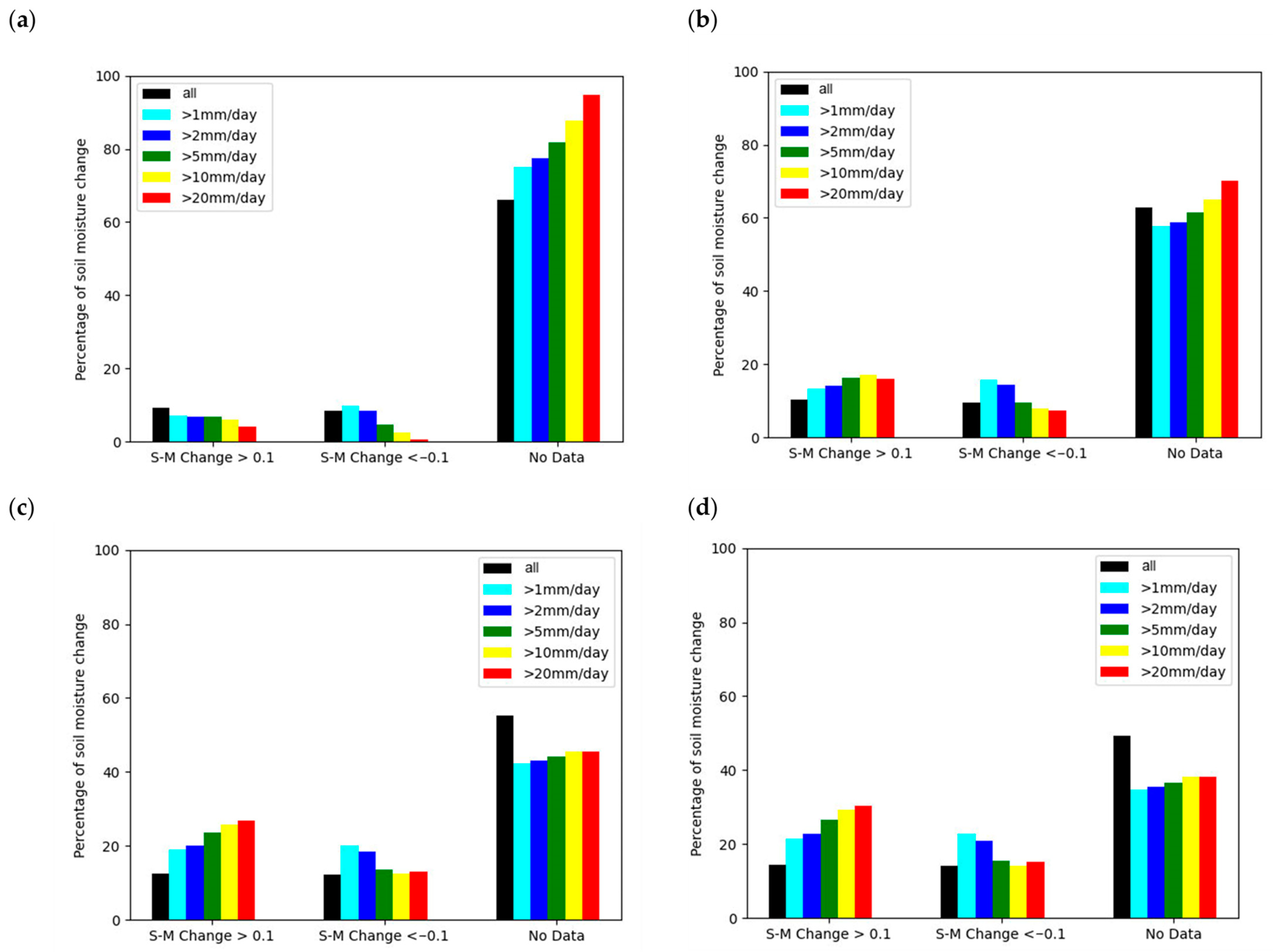
The soil moisture data used for this analysis is based upon the Thermal-Optical Trapezoid Method (TOTRAM) (Yang et al. [23]), which combines satellite-based land surface temperature (LST) and normalized difference vegetation index (NDVI) observations. The LST serves as a proxy for the moisture conditions in the soil. Water in the soil cools its surroundings through evaporation and transpiration. When the LST is equal to the air temperature, a large part of the energy of the incoming radiation is used for evapotranspiration processes, which indicates well-watered conditions. If the LST is significantly higher than the air temperature, the surface is not cooled due to evapotranspiration, which means that a crop is stressed because it is not able to retrieve enough water from the soil or that the topsoil is too dry to evaporate. To account for the effect of vegetation cover (Fc) on the LST caused by the change in albedo and the shading of the topsoil, the NDVI is used. The result is an LST-Fc trapezoidal space, where the soil wetness isolines between the theoretical upper (warm) edge and lower (cold) edge can be converted to a relative soil moisture content given the instantaneous LST and NDVI observations. Figure 4 shows a schematic of the trapezoidal space of the TOTRAM model.

This soil moisture model is incorporated into the ETLook model (Bastiaanssen et al. [31]) as a stress component for calculating evapotranspiration, mostly because of the relatively high spatial resolution (10 m) of Sentinel-2 based NDVI data. Although VIIRS-based LST data has a lower resolution of 375 m, we used an NDVI-based thermal sharpening method (Gao et al. [32]) to downscale the VIIRS data to the same 10 m grid. An added benefit of using the TOTRAM model within ETLook is the ability to calibrate the trapezoidal space on a pixel level. In contrast to the method described by Yang et al. [23], ETLook uses the wet bulb temperature (WBT) to determine the cold edge to improve the model performance for arid climates.

Alternative radar-based soil moisture models only provide data at a 500 m spatial resolution or lower (Massari et al. [33], Zappa et al. [34], and Dari et al. [35]), which is insufficient for modeling evapotranspiration at 10 m resolution. An added benefit is that the TOTRAM soil moisture model estimates soil moisture for the entire rooting depth, in contrast to the topsoil (~5 cm) observations of radar-based soil moisture models, which is highly valuable for calculating the moisture stress component of the vegetation.

However, when using soil moisture data to improve the spatial accuracy of precipitation data, observations from the topsoil are preferred. If soil moisture is observed at the rooting depth, the precipitation signal is attenuated. However, if the rooting depth is shallow or the soil is bare, the attenuation of the precipitation signal should be limited, similar to radar-based soil moisture data. For this research, the default soil moisture dataset of 10 m resolution was split into two scenarios: (1) soil moisture observations at rooting depth (default) and (2) soil moisture observations for bare soil conditions. For both scenarios, the 10 m resolution soil moisture data are mapped to a 1 km grid. For scenario 1, the mapping approach was to calculate the mean of all the soil moisture values of the pixels within the 1 km grid. For scenario 2, first, the pixels where significant vegetation cover persisted (NDVI > 0.3) were removed. Second, any pixels which could represent standing water (NDVI < 0.1) were also removed. Lastly, for the remaining pixels, the mean over the same 1 km grid was calculated. Additionally, a record was held of how many pixels satisfied the filter criteria to prevent using unrepresentative data at the 1 km grid scale.

6.2. Results

When possible, the data from consecutive days are used to calculate the soil moisture change. This resulted in an overall data availability ranging from 2.3% in forested areas to 53.3% in areas with less vegetation (Figure 5). To investigate the effect of the vegetation filter on the data availability, the soil moisture change was also calculated from the unfiltered data, which gave a similar result with a substantial increase in data availability only in densely vegetated areas in the west and southeast of the domain.

To overcome these issues, longer timesteps were allowed, e.g., if no soil moisture information was available, the soil moisture difference was calculated with respect to the last day that had data. Gaps of up to 4 days were allowed initially only for entire images (not shown) and later also on the basis of individual pixels (Figure 6). The former only had a small effect on data availability, and even though the latter resulted in an overall increase in data availability, it still remained below 63%. To further increase the data availability, a reverse speckle filter was applied to identify spatial gaps in the data and fill them by interpolating over neighboring pixels. Gaps of up to 100 pixels were treated in this way. This resulted in an increased and more homogeneous data availability with values up to 65%. It should be noted that all the measures to increase the data availability, namely using unfiltered data with respect to vegetation, including longer timesteps and applying a reverse speckle filter, potentially lead to a less direct relationship between the inferred soil moisture change and precipitation events.

Therefore, the relationship between the soil moisture change of the topsoil (scenario 2) and the cumulated precipitation was investigated. For this purpose, the cumulated precipitation was calculated between the dates that were used to calculate the soil moisture change for individual pixels. The cumulated precipitation was grouped according to the precipitation amount with the expectation that more precipitation would increase the chance of a positive soil moisture change and decrease the chance of a negative one. Unfortunately, when looking at Figure 7a, the most prominent feature is the increase in missing soil moisture change data for periods with large precipitation amounts, e.g., for cumulated precipitation of more than 20 mm, 95% of the soil moisture data were missing. The likelihood of observing a positive soil moisture change was only 9.5%, irrespective of the precipitation, and decreased to about 3.5% for precipitation sums larger than 20 mm. Observing a decrease in relative soil moisture was equally unlikely, and the percentage of these cases decreased further with increasing precipitation down to about 1% for precipitation sums larger than 20 mm. The poor data availability is likely because the soil moisture data tends to be missing for days with large precipitation sums, which can be explained by the inability of the sensor to measure through clouds. When allowing missing images for up to four days when calculating the soil moisture change, the increase in missing data with precipitation amounts is slightly less pronounced, e.g., for cumulated precipitation of more than 20 mm, 70% of the soil moisture data were missing. A positive soil moisture change is slightly more likely for periods with large precipitation sums, e.g., for cumulated precipitation of more than 20 mm, 16% of the relative soil moisture data showed an increase larger than 0.1. (Figure 7b). Allowing gaps of up to four days for individual pixels further reduces the increase in missing data for more precipitation (46% missing data for precipitation sums larger than 20 mm) and also makes positive soil moisture changes more likely for larger precipitation sums, e.g., for cumulated precipitation of more than 20 mm, 27% of the relative soil moisture data showed an increase larger than 0.1. (Figure 7c). Additionally, reducing the gaps via a reverse speckle filter increases the data availability slightly but otherwise does not change the analysis significantly, as this is also the case for the observations of negative soil moisture change. Overall, this analysis is still dominated by missing data, and while a stronger relationship between a positive soil moisture change and larger precipitation amounts could be achieved through the different processing steps, there are also still many cases with a negative soil moisture change despite large precipitation amounts in the considered period, e.g., in Figure 7d for cumulated precipitation of more than 2 mm, 21% of the relative soil moisture data showed a decrease larger than 0.1.

In a different approach, the condition on vegetation was relaxed, and all soil moisture data were considered in calculating the soil moisture change (scenario 1). On this basis, the soil moisture changes were calculated again, allowing gaps of up to 4 days on an individual pixel basis. However, the results inferred in this way looked less promising than the ones for topsoil only. Allowing gaps in the soil moisture data when calculating the soil moisture changes implicitly increases the delay of the soil moisture data by the length of the gaps that are allowed in the process.

6.3. Individual Cases

Apart from the obvious problem with missing data, the soil moisture change data also show:

• other signals not related to precipitation;
• relatively weak to no signals for periods with significant precipitation events.

To improve our understanding of this behavior, we looked at three cases in more detail.

In the first case, large precipitation amounts of up to 80 mm were measured in some parts of the domain, while the major part of the domain received much less rain, with values between 0.01 mm and 8 mm (Figure 8d). The soil moisture change data calculated from unfiltered relative soil moisture data of consecutive days again features many areas with missing data, but also for regions with partial data coverage in the southern part of the domain, no pattern resembling the precipitation distribution could be detected (Figure 8a). Most of the data going into this image originate from the root zones of plants within the domain, which is likely to introduce a delay between precipitation and soil moisture. However, calculating the soil moisture change for topsoil only resulted in a very similar image (Figure 8b). Seeing the similarity between these two images gave rise to the hypothesis that the images are dominated by factors other than recent precipitation events. In an attempt to recover the precipitation signal, the soil moisture change as the difference of root zone and topsoil relative soil moisture was calculated (Figure 8c). However, despite showing a more positive soil moisture change, the precipitation pattern also cannot be recognized in this image.

In contrast to the first case, the second one shows a very distinct pattern in the soil moisture change data calculated from all soil depths and from topsoil only (Figure 9a,b). However, in this period, no significant precipitation was recorded in the entire domain (Figure 9d). The soil moisture change calculated from the difference of topsoil and root zone successfully removes the majority of this signal resulting in only weak positive soil moisture change with the largest values in the southwestern part of the domain (Figure 9c).

The third case features patches with and without soil moisture change data distributed over the entire domain, with more data available in the western part (Figure 10). The soil moisture changes calculated from scenario 1 as well as scenario 2 feature predominantly positive values in the northwestern part of the domain and gradually decrease and eventually become negative towards the southeast. This nicely matches the general distribution of the precipitation over this period (Figure 10d). Calculating the soil moisture change based on the difference between topsoil and root zone soil, in this case, leads to a plot with patches of slightly positive and slightly negative values relatively evenly distributed over the area under consideration (Figure 10c).

Figure 8, Figure 9 and Figure 10 show that using LST-NDVI-based soil moisture data does not add much value to downscaling IMERG Late precipitation data. Naturally, cloud cover during precipitation events prohibits the satellites from observing the land surface. The likelihood of the availability of two cloud-free images just before and after a precipitation event is low at best. Although Figure 10 shows some signs of a positive correlation between an increase in soil moisture content after a precipitation event, the gaps in the entire time series, as well as in the individual images, make it currently impossible to reliably downscale satellite-based precipitation data using this soil moisture dataset.

However, some confusing patterns in soil moisture change are not caused by the soil moisture model itself but are introduced due to artifacts in the satellite data. For example, Figure 9 shows a relatively strong soil moisture increase in the left part of the image, while no precipitation was recorded. When comparing the raw LST data from VIIRS to the soil moisture change pattern at high resolution (Figure 11), it becomes clear that the increase in soil moisture is a result of an inaccurate cloud mask. The default cloud mask from VIIRS, which was used for this product, is unable to remove shadows or hazy pixels from this image, which have significantly lower LST values than cloud-free pixels. Since lower LST values correspond to wetter soil moisture conditions at the same NDVI, the model assumes that there is an increase in soil moisture content. Having a more accurate cloud mask would result in fewer artifacts and a stronger correlation between the soil moisture change and precipitation flux. However, a better cloud mask inherently also means fewer observations, which negatively impacts the temporal resolution and, thus, the usability of this dataset for downscaling satellite-based precipitation data, such as IMERG late.

6.4. Alternative Datasets for Downscaling

Alternatively, other soil moisture datasets could be considered, such as SMOS, which has already successfully been used by Pellarin et al. [3], Brocca et al. [4], and Brocca et al. [13]. However, this would mean that the spatial resolution would be much lower, e.g., 0.25° in the case of SMOS. Thus, it would not be able to improve the spatial resolution of IMERG late data. Many efforts have been made to downscale low-resolution microwave-based soil moisture data (Massari et al. [33]). However, the use case of downscaling precipitation data demands daily soil moisture observations at a high resolution (1 km), which currently does not exist on a global scale. For example, multiple approaches exist to retrieve high-resolution (< 1km) soil moisture data based on Sentinel-1 observations. However, Sentinel-1 does not observe the globe in an evenly distributed manner, resulting in an insufficient temporal resolution over Australia (Fourcras et al. [36] and Bauer et al. [37]).

7. Conclusions

A high-quality gridded precipitation dataset, based on radar and rain gauge data, was derived for the Namoi catchment. This dataset was used as a testbed to investigate different satellite-based multi-instrument precipitation data such as GSMaP and IMERG, as well as the reanalysis data ERA5. The quality of these globally available datasets was assessed with the requirements of WaterSENSE in mind. IMERG late data were found to be the best data to complement gauge-adjusted radar data for areas in Australia where these data are not available. The testbed was also used to improve our understanding of the relationship between precipitation and a state-of-the-art relative soil moisture dataset also produced in this project. The idea was that the high-resolution soil moisture data could be used to downscale the coarser-resolution satellite-based precipitation data. A general relationship between a positive soil moisture change and large precipitation events in the same period could be shown. Moreover, different methods were successfully tried to mitigate the effect of missing soil moisture data both temporally and spatially. However, as can be seen from Figure 7 as well as from the individual case studies, the fraction of missing data is too high to continue to implement this method for downscaling the satellite-based precipitation data. Even in the third individual case, where a general agreement between the soil moisture and the precipitation pattern exists, the patchiness of the data prohibits its application in this context. Additionally, the soil moisture change data sometimes do not reflect strong precipitation events (case one) and show strong signals not related to precipitation in other situations (case two). The detailed investigation of these cases improved our understanding of the complexity between data availability and data applicability for these interesting situations.

Given the above analysis, IMERG late data in its original form was chosen as precipitation data in WaterSENSE for regions with insufficient radar and rain gauge coverage. This enables us to provide precipitation data for the whole of Australia independently of the density of the gauge network.

References

1. Einfalt, T.; Frerk, I. On the influence of high quality rain gauge data for radar-based rainfall estimation. In Proceedings of the 12th ICUD, Porto Alegre, Brazil, 11–16 September 2011. [Google Scholar]
2. Willems, P.; Einfalt, T. Sensors for rain measurements. Metrol. Urban Drain. Stormwater Manag. Plug Pray. 2021, 11, 11–33. [Google Scholar] [CrossRef]
3. Pellarin, T.; Román-Cascón, C.; Baron, C.; Bindlish, R.; Brocca, L.; Camberlin, P.; Fernández-Prieto, D.; Kerr, Y.H.; Massari, C.; Panthou, G.; et al. The Precipitation Inferred from Soil Moisture (PrISM) Near Real-Time Rainfall Product: Evaluation and Comparison. Remote Sens. 2020, 12, 481. [Google Scholar] [CrossRef] [Green Version]
4. Brocca, L.; Pellarin, T.; Crow, W.T.; Ciabatta, L.; Massari, C.; Ryu, D.; Su, C.-H.; Rüdiger, C.; Kerr, Y. Rainfall estimation by inverting SMOS soil moisture estimates: A comparison of different methods over Australia. J. Geophys. Res. Atmos. 2016, 121, 12062–12079. [Google Scholar] [CrossRef]
5. He, K.; Zhao, W.; Brocca, L.; Quintana-Seguí, P. SMPD: A soil moisture-based precipitation downscaling method for high-resolution daily satellite precipitation estimation. Hydrol. Earth Syst. Sci. 2023, 27, 169–190. [Google Scholar] [CrossRef]
6. Chen, C.; Chen, Q.; Qin, B.; Zhao, S.; Duan, Z. Comparison of different methods for spatial downscaling of GPM IMERG V06B satellite precipitation product over a typical arid to semi-arid area. Front. Earth Sci. 2020, 8, 536337. [Google Scholar] [CrossRef]
7. Pellarin, T.; Ali, A.; Chopin, F.; Jobard, I.; Bergès, J.C. Using spaceborne surface soil moisture to constrain satellite precipitation estimates over West Africa. Geophys. Res. Lett. 2008, 35. [Google Scholar] [CrossRef] [Green Version]
8. Jackson, T.J.; Cosh, M.H.; Bindlish, R.; Starks, P.J.; Bosch, D.D.; Seyfried, M.; Goodrich, D.C.; Moran, M.S.; Du, J.Y. Validation of advanced microwave scanning radiometer soil moisture products. IEEE Trans. Geosci. Remote Sens. 2010, 48, 4256–4272. [Google Scholar] [CrossRef]
9. Crow, W.T.; Huffman, G.J.; Bindlish, R.; Jackson, T.J. Improving satellite-based rainfall accumulation estimates using spaceborne surface soil moisture retrievals. J. Hydrometeorol. 2009, 10, 199–212. [Google Scholar] [CrossRef] [Green Version]
10. Kerr, Y.H.; Waldteufel, P.; Richaume, P.; Wigneron, J.P.; Ferrazzoli, P.; Mahmoodi, A.; Al Bitar, A.; Cabot, F.; Gruhier, C.; Delwart, S.; et al. The SMOS soil moisture retrieval algorithm. IEEE Trans. Geosci. Remote Sens. 2012, 50, 1384–1403. [Google Scholar] [CrossRef]
11. Brocca, L.; Moramarco, T.; Melone, F.; Wagner, W. A new method for rainfall estimation through soil moisture observations. Geophys. Res. Lett. 2013, 40, 853–858. [Google Scholar] [CrossRef]
12. Wagner, W.; Hahn, S.; Kidd, R.; Melzer, T.; Bartalis, Z.; Hasenauer, S.; Figa-Saldaña, J.; De Rosnay, P.; Jann, A.; Schneider, S.; et al. The ASCAT Soil Moisture Product: A Review of its specifications, validation results, and emerging applications. Meteorol. Z. 2013, 22, 5–33. [Google Scholar] [CrossRef] [Green Version]
13. Brocca, L.; Ciabatta, L.; Massari, C.; Moramarco, T.; Hahn, S.; Hasenauer, S.; Kidd, R.; Dorigo, W.; Wagner, W.; Levizzani, V. Soil as a natural rain gauge: Estimating global rainfall from satellite soil moisture data. J. Geophys. Res. Atmos. 2014, 119, 5128–5141. [Google Scholar] [CrossRef]
14. Schamm, K.; Ziese, M.; Becker, A.; Finger, P.; Meyer-Christoffer, A.; Schneider, U.; Schröder, M.; Stender, P. Global gridded precipitation over land: A description of the new GPCC First Guess Daily product. Earth Syst. Sci. Data 2014, 6, 49–60. [Google Scholar] [CrossRef] [Green Version]
15. Huffman, G.J.; Bolvin, D.T.; Nelkin, E.J.; Wolff, D.B.; Adler, R.F.; Gu, G.; Hong, Y.; Bowman, K.P.; Stocker, E.F. The TRMM multisatellite precipitation analysis (TMPA): Quasi-global, multiyear, combined-sensor precipitation estimates at fine scales. J. Hydrometeorol. 2007, 8, 38–55. [Google Scholar] [CrossRef]
16. Huffman, G.J.; Adler, R.F.; Bolvin, D.T.; Nelkin, E.J. The TRMM multi-satellite precipitation analysis (TMPA). In Satellite Rainfall Applications for Surface Hydrology; Springer: Dordrecht, The Netherlands, 2010; pp. 3–22. [Google Scholar]
17. Zhao, W.; Wen, F.; Wang, Q.; Sanchez, N.; Piles, M. Seamless downscaling of the ESA CCI soil moisture data at the daily scale with MODIS land products. J. Hydrol. 2021, 603, 126930. [Google Scholar] [CrossRef]
18. Crow, W.T.; van den Berg, M.J.; Huffman, G.J.; Pellarin, T. Correcting rainfall using satellite-based surface soil moisture retrievals: The Soil Moisture Analysis Rainfall Tool (SMART). Water Resour. Res. 2011, 47. [Google Scholar] [CrossRef]
19. Massari, C.; Camici, S.; Ciabatta, L.; Brocca, L. Exploiting satellite-based surface soil moisture for flood forecasting in the Mediterranean area: State update versus rainfall correction. Remote. Sens. 2018, 10, 292. [Google Scholar] [CrossRef] [Green Version]
20. Brocca, L.; Melone, F.; Moramarco, T. Distributed rainfall-runoff modelling for flood frequency estimation and flood forecasting. Hydrol. Process. 2011, 25, 2801–2813. [Google Scholar] [CrossRef]
21. Sadeghi, M.; Babaeian, E.; Tuller, M.; Jones, S.B. The optical trapezoid model: A novel approach to remote sensing of soil moisture applied to Sentinel-2 and Landsat-8 observations. Remote. Sens. Environ. 2017, 198, 52–68. [Google Scholar] [CrossRef] [Green Version]
22. Bai, L.; Long, D.; Yan, L. Estimation of surface soil moisture with downscaled land surface temperatures using a data fusion approach for heterogeneous agricultural land. Water Resour. Res. 2019, 55, 1105–1128. [Google Scholar] [CrossRef]
23. Yang, Y.; Guan, H.; Long, D.; Liu, B.; Qin, G.; Qin, J.; Batelaan, O. Estimation of surface soil moisture from thermal infrared remote sensing using an improved trapezoid method. Remote. Sens. 2015, 7, 8250–8270. [Google Scholar] [CrossRef] [Green Version]
24. NSW Department of Planning, Industry and Environment. Draft Regional Water Strategy—Namoi: Strategy. 2021. Available online: https://www.industry.nsw.gov.au/__data/assets/pdf_file/0009/354267/namoi-strategy.pdf (accessed on 17 September 2021).
25. Kubota, T.; Aonashi, K.; Ushio, T.; Shige, S.; Takayabu, Y.N.; Kachi, M.; Arai, Y.; Tashima, T.; Masaki, T.; Kawamoto, N.; et al. Global Satellite Mapping of Precipitation (GSMaP) Products in the GPM Era. In Satellite Precipitation Measurement. Advances in Global Change Research; Levizzani, V., Kidd, C., Kirschbaum, D., Kummerow, C., Nakamura, K., Turk, F., Eds.; Springer: Cham, Switzerland, 2020; Volume 67, pp. 355–373. [Google Scholar] [CrossRef]
26. Huffman, G.J.; Bolvin, D.T.; Braithwaite, D.; Hsu, K.; Joyce, R.; Xie, P.; Yoo, S.H. Algorithm Theoretical Basis Document (ATBD) Version 06. NASA Global Precipitation Measurement (GPM) Integrated Multi-Satellite Retrievals for GPM (IMERG). 2019. Available online: https://pmm.nasa.gov/data-access/downloads/gpm (accessed on 4 December 2019).
27. Hersbach, H.; Bell, B.; Berrisford, P.; Hirahara, S.; Horányi, A.; Muñoz-Sabater, J.; Simmons, A.; Soci, C.; Bidlot, J.; Thépaut, J.N.; et al. The ERA5 global reanalysis. Q. J. R. Meteorol. Soc. 2020, 146, 1999–2049. [Google Scholar] [CrossRef]
28. Strehz, A.; Einfalt, T. Precipitation Data Retrieval and Quality Assurance from Different Data Sources for the Namoi Catchment in Australia. Geomatics 2021, 1, 417–428. [Google Scholar] [CrossRef]
29. Taylor, K.E. Summarizing multiple aspects of model performance in a single diagram. J. Geophys. Res. Atmos. 2001, 106, 7183–7192. [Google Scholar] [CrossRef]
30. Roberts, N.M.; Lean, H.W. Scale-selective verification of rainfall accumulations from high-resolution forecasts of convective events. Mon. Weather. Rev. 2008, 136, 78–97. [Google Scholar] [CrossRef] [Green Version]
31. Bastiaanssen, W.G.M.; Cheema, M.J.M.; Immerzeel, W.W.; Miltenburg, I.J.; Pelgrum, H. Surface energy balance and actual evapotranspiration of the transboundary Indus Basin estimated from satellite measurements and the ETLook model. Water Resour. Res. 2012, 48. [Google Scholar] [CrossRef] [Green Version]
32. Gao, F.; Kustas, W.P.; Anderson, M.C. A data mining approach for sharpening thermal satellite imagery over land. Remote. Sens. 2012, 4, 3287–3319. [Google Scholar] [CrossRef] [Green Version]
33. Massari, C.; Modanesi, S.; Dari, J.; Gruber, A.; De Lannoy, G.J.; Girotto, M.; Quintana-Seguí, P.; Le Page, M.; Jarlan, L.; Brocca, L.; et al. A review of irrigation information retrievals from space and their utility for users. Remote Sens. 2021, 13, 4112. [Google Scholar] [CrossRef]
34. Zappa, L.; Schlaffer, S.; Bauer-Marschallinger, B.; Nendel, C.; Zimmerman, B.; Dorigo, W. Detection and quantification of irrigation water amounts at 500 m using sentinel-1 surface soil moisture. Remote. Sens. 2021, 13, 1727. [Google Scholar] [CrossRef]
35. Dari, J.; Quintana-Seguí, P.; Escorihuela, M.J.; Stefan, V.; Brocca, L.; Morbidelli, R. Detecting and mapping irrigated areas in a Mediterranean environment by using remote sensing soil moisture and a land surface model. J. Hydrol. 2021, 596, 126129. [Google Scholar] [CrossRef]
36. Foucras, M.; Zribi, M.; Albergel, C.; Baghdadi, N.; Calvet, J.-C.; Pellarin, T. Estimating 500-m resolution soil moisture using Sentinel-1 and optical data synergy. Water 2020, 12, 866. [Google Scholar] [CrossRef] [Green Version]
37. Bauer-Marschallinger, B.; Freeman, V.; Cao, S.; Paulik, C.; Schaufler, S.; Stachl, T.; Modanesi, S.; Massari, C.; Ciabatta, L.; Brocca, L.; et al. Toward global soil moisture monitoring with Sentinel-1: Harnessing assets and overcoming obstacles. IEEE Trans. Geosci. Remote Sens. 2018, 57, 520–539. [Google Scholar] [CrossRef]
Figure 1. Map of the Namoi catchment and its surrounding. Depicted are the catchment (red line), the location of Namoi radar (black dot), the radar coverage after processing (radius of 240 km; black circle), the area used for the comparison of the different precipitation datasets with respect to spatial precipitation patterns (black rectangle) and the area used for the evaluation of the soil moisture data (blue rectangle).
Atmosphere 14 00435 g001
Figure 2. Catchment averaged daily (a) and hourly (b) precipitation of different near-global datasets compared against gauge-adjusted radar data using a Taylor diagram (Taylor [29]). The correlation is given by the angle to the y-axis (dashed lines). The standard deviation increases with distance to the origin of the coordinate system, and the standard deviation of the gauge-adjusted radar data is given as a reference (black arc). The root-mean-square error is given by the distance to the black dot on the x-axis (grey arcs).
Atmosphere 14 00435 g002
Figure 3. Spatial distribution of precipitation using fractions skill score (FSS). The datasets were analyzed over a square area of 200 km by 200 km centered on the location of the Namoi radar. Results are shown for two relative thresholds, the 0.75 quantile (a) and the 0.9 quantile (b), and for two fixed thresholds of 4 mm (c) and 16 mm (d).
Atmosphere 14 00435 g003
Figure 4. Trapezoidal LST-Fc space is used to derive the relative root zone soil moisture content (θ) based on satellite-based thermal (LST) and vegetation cover (Fc) data. The warm and cold edges of the trapezoid define at which LST and Fc value combination θ is equal to the residual moisture content (θR) or the field capacity (θF), respectively. Both the warm and cold edges are derived using meteorological data on a pixel level. Points A and B of the trapezoidal space define the warm edge using the maximum surface temperature of bare (Ts,max) and fully covered (Tc,max) pixels. Point C defines the cold edge of fully covered pixels using the minimum surface temperature (Ts,min). In contrast to Yang et al. [23], point D defines the cold edge of bare pixels using the wet bulb temperature (WBT) instead of the minimum surface temperature (Tc,min) to increase the accuracy of the model for bare soil conditions.
Atmosphere 14 00435 g004
Figure 5. Data availability of soil moisture change in percent calculated as the difference between the soil moisture of consecutive days for scenario 1 (a) and for scenario 2 (b).
Atmosphere 14 00435 g005
Figure 6. Data availability of soil moisture change in percent calculated as the difference between the soil moisture of consecutive days, for which soil moisture was available if the gap with no soil moisture data was shorter than five days for individual pixels (a). A reverse speckle filter was additionally applied to data to interpolate gaps of up to 100 pixels (b).
Atmosphere 14 00435 g006
Figure 7. Change of relative soil moisture for different precipitation sums. As a reference, the total percentage of pixels that falls into the three relative soil moisture change categories irrespective of the precipitation is also given as ‘all’. (a): The soil moisture change was calculated from consecutive days. (b): The soil moisture change was calculated allowing gaps of up to four days but uniform for the entire domain. (c): The soil moisture change was calculated allowing gaps of up to four days individually for every pixel. (d): Same as lower left, but a reverse speckle filter interpolating gaps of up to 100 pixels was applied to the data.
Atmosphere 14 00435 g007
Figure 8. Relative soil moisture change (dimensionless) calculated as the difference between consecutive days of relative soil moisture for scenario 1 (a), for scenario 2 (b), and from the difference between scenario 1 and 2 (c) for 29/10/2020. Positive values mean an increase in soil moisture, while negative values mean a decrease in soil moisture. Additionally, the respective cumulated radar precipitation is shown (d).
Atmosphere 14 00435 g008
Figure 9. Relative soil moisture change (dimensionless) calculated as the difference between consecutive days of relative soil moisture for scenario 1 (a), for scenario 2 (b), and from the difference between scenario 1 and 2 (c) for 04/11/2022. Positive values mean an increase in soil moisture, while negative values mean a decrease in soil moisture. Additionally, the respective cumulated radar precipitation is shown (d).
Atmosphere 14 00435 g009
Figure 10. Relative soil moisture change (dimensionless) calculated as the difference between consecutive days of relative soil moisture for scenario 1 (a), for scenario 2 (b), and from the difference between scenario 1 and 2 (c) for 22 January 2021. Positive values mean an increase in soil moisture, while negative values mean a decrease in soil moisture. Additionally, the respective cumulated radar precipitation is shown (d).
Atmosphere 14 00435 g010
Figure 11. Comparison between cloud-masked VIIRS-based LST data (a) and the difference between the high-resolution soil moisture data (b) for the 4th of November 2020. White parts of the image are masked using VIIRS’ standard cloud mask. At the edges of this cloud mask, significantly lower LST values are visible, presumably caused by unmasked clouds or cloud shadows, negatively impacting the performance of the soil moisture change product for downscaling precipitation data.
Atmosphere 14 00435 g011