Article

Harmonic Analysis of the Relationship between GNSS Precipitable Water Vapor and Heavy Rainfall over the Northwest Equatorial Coast, Andes, and Amazon Regions

by
Sheila Serrano-Vincenti
1,*,
Thomas Condom
2,
Lenin Campozano
3,4,
León A. Escobar
5,
Andrea Walpersdorf
6,
David Carchipulla-Morales
3 and
Marcos Villacís
3,4,*
1
Carrera de Ingeniería Ambiental, Grupo de Investigación en Ciencias Ambientales GRICAM, Centro de Investigación en Modelamiento Ambiental CIMA-UPS, Universidad Politécnica Salesiana, Quito 170105, Ecuador
2
IRD, CNRS, Grenoble INP, Institut de Geosciences de l’Environnement (IGE), Université Grenoble Alpes, 38 058 Grenoble, France
3
Departamento de Ingeniería Civil y Ambiental & Centro de Investigación y Estudios en Ingeniería de los Recursos Hídricos, Escuela Politécnica Nacional, Quito 170525, Ecuador
4
Grupo de investigación MetClimA, Escuela Politécnica Nacional, Quito 170517, Ecuador
5
Hydrological & Meteorological Division, Synaptronics, Columbia, MD 21046, USA
6
University Grenoble Alpes, University Savoie Mont Blanc, CNRS, IRD, University Gustave Eiffel, ISTerre, 38 400 Grenoble, France
*
Authors to whom correspondence should be addressed.
Atmosphere 2022, 13(11), 1809; https://doi.org/10.3390/atmos13111809
Submission received: 16 August 2022 / Revised: 18 October 2022 / Accepted: 26 October 2022 / Published: 31 October 2022

Abstract

:
This study finds the relationship between increases in precipitable water vapor (PWV), and intense rainfall events in four different climatological regions of South America’s equatorial northwest: the coast, Andes valley, high mountains, and Amazon. First, the PWV was derived from tropospheric zenith delay measured by Global Navigation Satellite System (GNSS) instrumentation located near meteorological stations within the regions of interest using hourly data from the year 2014. A harmonic analysis approach through continuous wavelet cross-spectrum and coherence, as well as discrete wavelets, was used to determine a measure of the lags found between PWV and specific heavy rain events and then compared with satellite IR images and meteorological anomalies. The link between PWV peaks and rainfall was the most evident on the coast, and less discernible in the other stations possibly due to local dynamic factors. The results showed a lag of 11 h between the preceding PWV increase and an intense rainfall event. This was apparent in all of the stations, except in Amazon where it was 6 h, with the highest precision at the coast and with the largest dispersion in the high mountains. The interpretation of this lag for each region is also discussed.

1. Introduction

The latest technological advances for meteorological applications based on GNSS (Global Navigation Satellite Systems) have received increased attention from the scientific community due to their availability in all types of atmospheric conditions, providing high temporal resolution, reliability, accuracy of the data, being a low-cost solution for the analysis, modeling, and forecasting of extreme rainfall events [1,2].
The GNSS signals characterize the atmosphere as they pass through it, related to the conditions of the pressure, temperature, and humidity of the troposphere. The troposphere generates variable delays (ZTD for Zenit Total Delay) that can be quantified in the GNSS analysis [3,4]. This is how the term “GPS Meteorology” is used, which is based on two techniques: the first uses ground-based geodetic GNSS stations (GB-GNSS in this work) that indicate the amount of tropospheric water vapor (PWV for Precipitable Water Vapor, TPW for Total Precipitable Water or IWV for Integrated Water Vapor) precisely over the GNSS station [5]. If the GB-GNSS station network is sufficiently dense, it is possible to know the vertical structure of the troposphere through tomographic reconstructions [6,7,8]. The second is a remote sensing technique called RO-GNSS (RO for Radio-occultation), which measures from a Low Earth Orbit (LEO) satellite the refraction effect of the signal of a GNSS satellite rising or settling behind the Earth. This measurement provides vertical profiles of the structure of the Earth’s atmosphere. Both techniques have been used in the study of intense rains, convective storms, tropical cyclones, atmospheric rivers, heat waves, and droughts [9,10].
The potential of these technologies has led to the generation of several international projects in the United States, Europe, and Asia that seek to improve the constellation of associated satellites, such as the Global Positioning System (GPS, USA), GLObal NAvigation Satellite System (GLONASS, Russia), Galileo (European Space Agency, Paris, France), and BeiDou (China), as well as improving the GB-GNSS network and associated real-time tropospheric devices. As a result, significant improvements have been reported in the forecasting of Numerical Weather Prediction (NWP) models, especially in severe weather conditions, by assimilating observed PWV data with high accuracy and high temporal resolution [11,12].
In this way, not only the modeling of intense rainfall events has been improved by PWV assimilation, but new relationships have also been found between PWV and rainfall characteristics. Several studies mention the occurrence of PWV thresholds [13,14] and/or peaks before heavy rain events [15]. Extreme rain is commonly defined as rain which exceeds high percentiles, 95th, 97th, or 99th, of the distribution of accumulated frequencies of daily precipitation, although this definition depends a lot on the climatic characteristics of the place [16]. Thus, investigations with hourly resolution data study windows of 6 h for the location of PWV peaks before intense rain events on the eastern coasts of China (at around 170 m above the sea level) [17,18], a 6 h window was also found in Lisbon, Portugal (~125 m.a.s.l.) [19,20], and 3 h windows in various locations in Italy [10]. Likewise, using finer resolutions (1 min) in Sao Paulo (Brazilian Amazon) (~85 m.a.s.l.), PWV peaks were found 32–36 min before heavy rain events [21], while lags of 4 and 8 h, respectively, between PWV peaks and shallow-to-deep convection transitions were reported [22]. Finally, researchers in the Argentina Valley of Mendoza (~769 m.a.s.l.), detected PWV increases before heavy storms but not a conclusive lag [23].
However, the evolution of the PWV time series is different for each reported case, both before and after the rainy event and no generalizations can be made about the time between the peak of PWV and the start of heavy rain [2]. In fact, all studies have reported significant increases in PWV that have not preceded any rain event, showing that the increase in PWV is just one more of the conditions for the generation of intense rain [19]. Therefore, it is necessary to analyze additional events in regions with contrasting climates and on complex topographies, in order to take into account the effect that altitude and different synoptic conditions may have on the behavior of the PWV; this us to help draw general conclusions regarding the establishment of critical PWV values or other dynamic indicators.
In this context, the present study has been conducted in Ecuador. Despite its small area, it has a diverse topography with three climatically different regions: the coast, the Andes, and the Amazon region. Additionally, it has a moderately dense network of GB-GNSS stations distributed at different altitudes, making it an ideal place to improve the understanding of the relationship of PWV with heavy rainfall events.
Note that previous studies conducted with GNSS-based meteorological applications in this area have been scarce and involve only daily or monthly resolutions [24,25]. The present research, in contrast, uses hourly resolutions to contribute to the understanding of the sub-diurnal dynamics of the aforementioned regions. It combines for this purpose a time-frequency harmonic analysis with statistical methods in the form of wavelet coherence and wavelet cross-spectrum analyses, while taking into consideration the dynamic and climatic characteristics of each region.

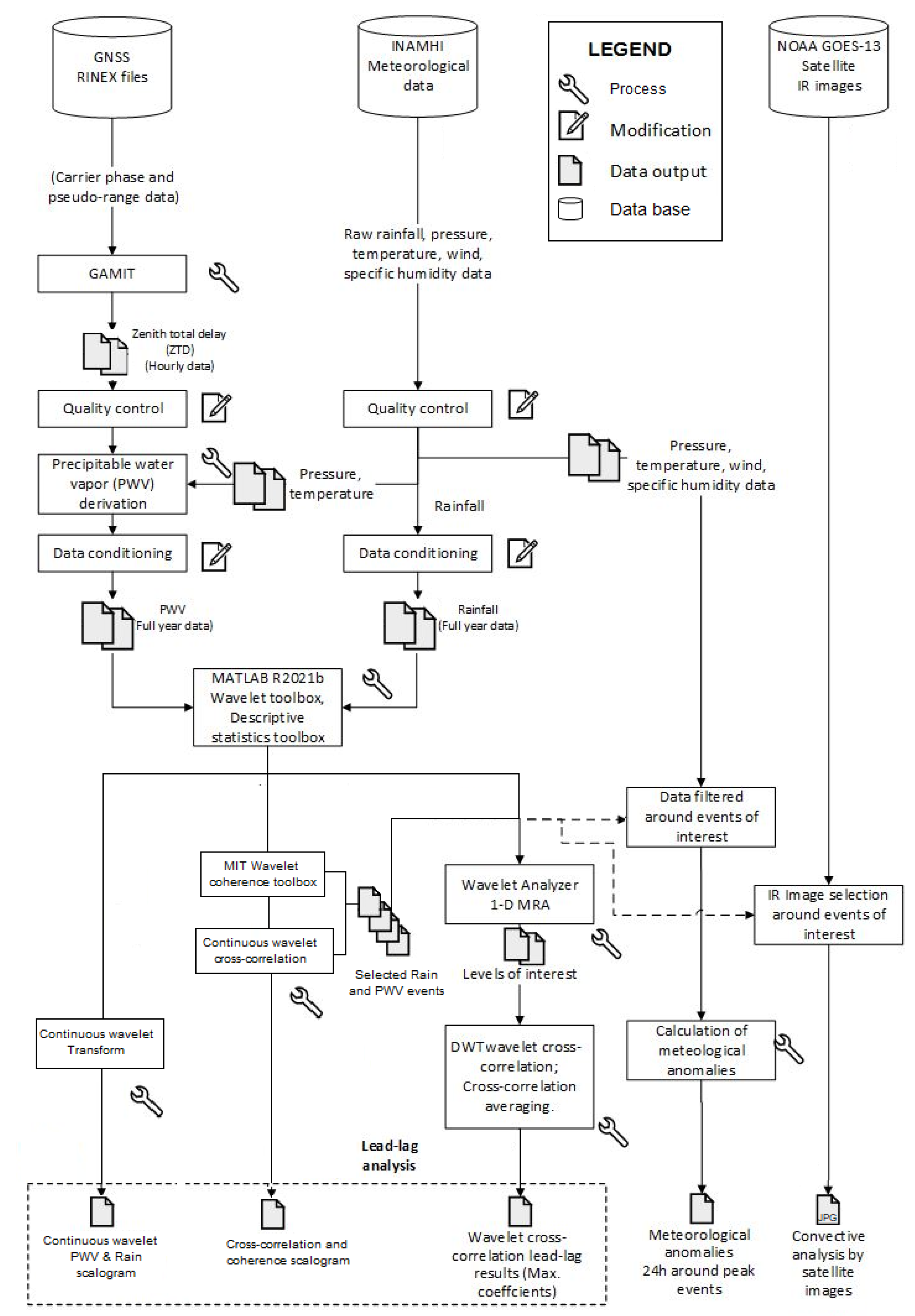
2. Geographical Location of the Measurement Network and Methods

2.1. GNSS-ZTD Data

Data used for the present analysis has been obtained from the National Geodetic Network RENGEO of the Geophysics Institute of the National Polytechnic School (Instituto Geofísico de la Escuela Politécnica Nacional IG-EPN) https://www.igepn.edu.ec/red-nacional-de-geodesia (accessed on 21 March 2019), which is continually updated in the database of UNAVCO https://www.unavco.org/data/gps-gnss/gps-gnss.html, accessed on 21 March 2019.
First, in this database, there were 17 stations that corresponded to the geographical regions of interest and had complete data allowing ZTD estimation with hourly resolutions. The selection was narrowed down to five sites, which were the ones close to meteorological stations with available hourly data for the year 2014. These GNSS-selected stations are located in the coastal region (SNLR), Andes region (BELI, IBEC, ASEC), and the Amazon region (TEN1) (See Figure 1). The location and technical specifications of these stations are found in Table 1 and Table 2, respectively.
After the selection process, the ZTD time series were estimated by processing the GNSS data using the GAMIT/GLOBK software [26].

2.2. Meteorological Data

Weather data from the year 2014 were obtained from locations close to the selected GNSS stations. These weather stations were sparse and managed by the National Institute of Meteorology and Hydrology of Ecuador (Instituto Nacional de Meteorología e Hidrología—INAHMI), in a particular case in cooperation with the French Institute of Research for Development (Institut de recherche pour le développement, IRD) [27], and by the Quito Atmospheric Monitoring Metropolitan Network (Red Metropolitana de Monitoreo Atmosférico de Quito—REMMAQ). Figure 1 shows the location of these weather and GPS stations on the map and Table 1 contains their geographic coordinates with additional information such as altitude, monitored weather parameters, a time resolution of the data, and distance to the closest GPS station.

2.3. Calculating ZTD from GNSS Data

The GNSS data processing is carried out through the GAMIT/GLOBK R10.7 software using a doubly differenced approach to eliminate clock errors from satellites and ground receivers in addition to a linear combination L3 (also called LC) of the GNSS phase signals in the L1 and L2 band to mitigate the errors introduced by the ionosphere. Only GPS data have been employed, as the receivers had no multi-GNSS capacities at the time of this study. Due to the fact that GAMIT determines the position of the GPS-GB stations with great accuracy and precision in order to quantify tectonic displacements, several models are taken into account for its computation, to separate tectonic deformation from other geophysical features. Modeled are for example the deformation of the earth’s crust due to the ocean tides, also known as ocean loading, atmospheric loading, and the influence of solar and lunar movements on Earth’s atmosphere (atmospheric tides) [26].
GAMIT parameterizes the ZTD as a stochastic variation of the Saastamoinen model, with a stepwise linear interpolation. The variation is calculated over a first-order Gauss–Markov process, with a potential density of 2 cm2/h, known as the “zenith restriction parameter”. A sliding window strategy is used to avoid offsets at the limits between two successive sessions in order to prevent day boundary discontinuities of the satellite orbits, e.g., [8]. Two 24 h sessions are calculated, starting at 0 h UTC and 12 h UTC, respectively. From both sessions, we keep the central 12 h to obtain a continuous well-constrained time series of ZTD for each station across the day boundary. The first and last 6 h of each analysis session are removed in order to take away the less well-constrained values at the session’s start and end while adjusting the final IGS orbits to smooth the day boundary discontinuity [28]. The GAMIT analysis producing these hourly ZTD values for each station was conducted at the Institute of Earth’s Sciences, ISTerre, of the University Grenoble Alpes, using the ISTerre computing cluster IST-OAR.

2.4. Quality Control and Data Synchronization

Once continuous ZTD data was obtained through the GAMIT sliding window analysis, repetitions of the values at session boundaries at 06:00 and 18:00 UTC, which account for 1% to 2% of the total data, were eliminated. In this way, it was possible to generate complete hourly ZTD series for the entire year 2014 at the Quito (Andes valley 1) and Antisana (High Mountain) stations. For the three remaining GB-GNSS stations, available data was found only from 21 July 2014 at 16:00 until the end of the year.
The quality of the hourly meteorological data from the in-situ stations required a thorough treatment, which was carried out on the available data series for each meteorological parameter rainfall: temperature, atmospheric pressure, wind speed, and relative humidity. The data series covered thirteen years for Antisana (High Mountain), seven years for Tena (Amazon), Esmeraldas (Coast) and Ibarra (Andes valley 2), and eight years for Quito (Andes valley 1). This amount of available data was used to determine the average values of the meteorological variables in order to determine the mean meteorology of the site presented in Section 3.1.
The quality control carried out for these meteorological data series was performed in accordance with the standards for hourly data treatment [29]. It was carried out first on the bias error, which corresponds to a discontinuity in the moving averages of the data, frequently due to the deviation of the sensors, which must be corrected by adding a constant value to the discontinuous period so that the moving averages are maintained [30].
Next, the extreme discontinuous values (outliers) were eliminated, defined as those values which were outside the interval [μ ± 4σ] [30], with the exception of the value of rainfall, which, being characterized by non-normal distributions [31,32] could present higher rainfall intensities. In this case, values greater than [μ + 10σ] were eliminated [33]. Once the outliers were eliminated, no padding was performed in these meteorological data.
Only in the case of the Antisana station (high mountain), the surface atmospheric pressure was estimated since it was not available in the corresponding weather station. The estimation used the time series of the surface atmospheric pressure of the Quito station instead (Andes valley 1), given its similar mean hourly homogenous behavior, but subtracting the value of 156.1 hPa, corresponding to the difference of the average pressures calculated by height differences [34] (Table 3).
Finally, the hourly time series of the ZTD was changed from UTC to local time, and common work periods were selected in order to synchronize the meteorological data with the ZTD.

2.5. Estimation of the PWV from the ZTD

The Total Zenith Delay ZTD depends on the refractivity that the GNSS signal encounters when crossing the atmosphere. This delay has two components: a Zenith Hydrostatic Delay ZHD due to a hydrostatic or total troposphere, which generally explains 90% of ZTD [35], and a wet component or Zenith Wet Delay ZWD due to the tropospheric water vapor, which is a strong variable and related to the PWV that explains the remaining 10% of the total delay. Equation (1) [3,4]:
Z T D = Z H D + Z W D
Z H D in [m] is obtained from the surface atmospheric pressure   P s in [hPa] by
Z H D = 2.2768 ± 0.0015 .10 5 P s / f θ , H
and,
f θ , H = 1 0.00266 c o s 2 θ 0.000279 H
where θ is the latitude, and H is the ellipsoidal height in [km]. Calculating ZHD from surface pressure and the station position, ZWD can be isolated in the ZTD measurement (Equation (1)). According to Bevis et al. [4], Z W D has a relationship with the P W V , given by:
P W V = κ Z W D
The κ constant depends on the vertical integral of the vapor density and the temperature, and it has a 2% precision [8]. In similar climatology studies, a κ E & D constant is used as presented by [36], which has a precision of 1.15% and has the advantage that it only depends on the surface temperature T s :
κ E & D = 10 3 6.324 0.0177   T s 289.76 + 0.000075   T s 289.76 2
Therefore, PWV can be estimated from GNSS ZTD measurements and meteorological ground pressure and temperature observations as in Equation (2):
P W V E & D = κ E & D Z W D

2.6. Conditioning of the Resulting PWV and Rain Data for Harmonic Analysis

Further analysis of the PWV and rain data required some data conditioning to assure the standardization and correct interpretation of the results while working with these two different magnitude time series: rainfall and PWV, using harmonic analysis tools.
The time series was normalized, dividing the values of the series by the maximum value recorded in order to preserve their original envelope, especially in the case of rainfall where sudden increases and the different intensities of the rainfall events where noticeable.
The choice of wavelets as the main tool to analyze these observables made it necessary to inspect if any incomplete or corrupted data was going to affect the periodicities of the series. Thus, the incomplete data were padded with linear interpolation in the case of PWV and with zeros in the case of rainfall, which correspond to the mode of this data. This padding was made between the available samples at each end of every empty (missing) piece of data in order to preserve the smoothness of the series rather than creating harsh discontinuities and, at the same time, minimizing the creation of artificial events. Figure 2 shows the time series of rain and PWV after conditioning per station. Regions padded with data are those marked with vertical gray lines.

2.7. Harmonic Analysis by Descriptive Statistics and Wavelets

The presented methodology uses the harmonic analysis of the time series via wavelets, a tool of great interest within applied mathematics that has allowed novel applications in several areas of knowledge, including those related to the study of natural phenomena [37,38,39]. The intrinsic relationship between time and frequency helps us to obtain information from rainfall and PWV data by visualizing the elementary atoms, or values of interest that are well concentrated in time and frequency, the variability of the signals, the analysis with various levels of detail of the signals by means of a change of scale (zooming) of time or frequency, and the characterization of signal structures such as singularities [40].
Additionally, it is recommended to read [41,42] for a deeper understanding of this tool. Note that the wavelet and statistical analysis was performed in Matlab R2021a [43] using built-in and third-party libraries as described later.

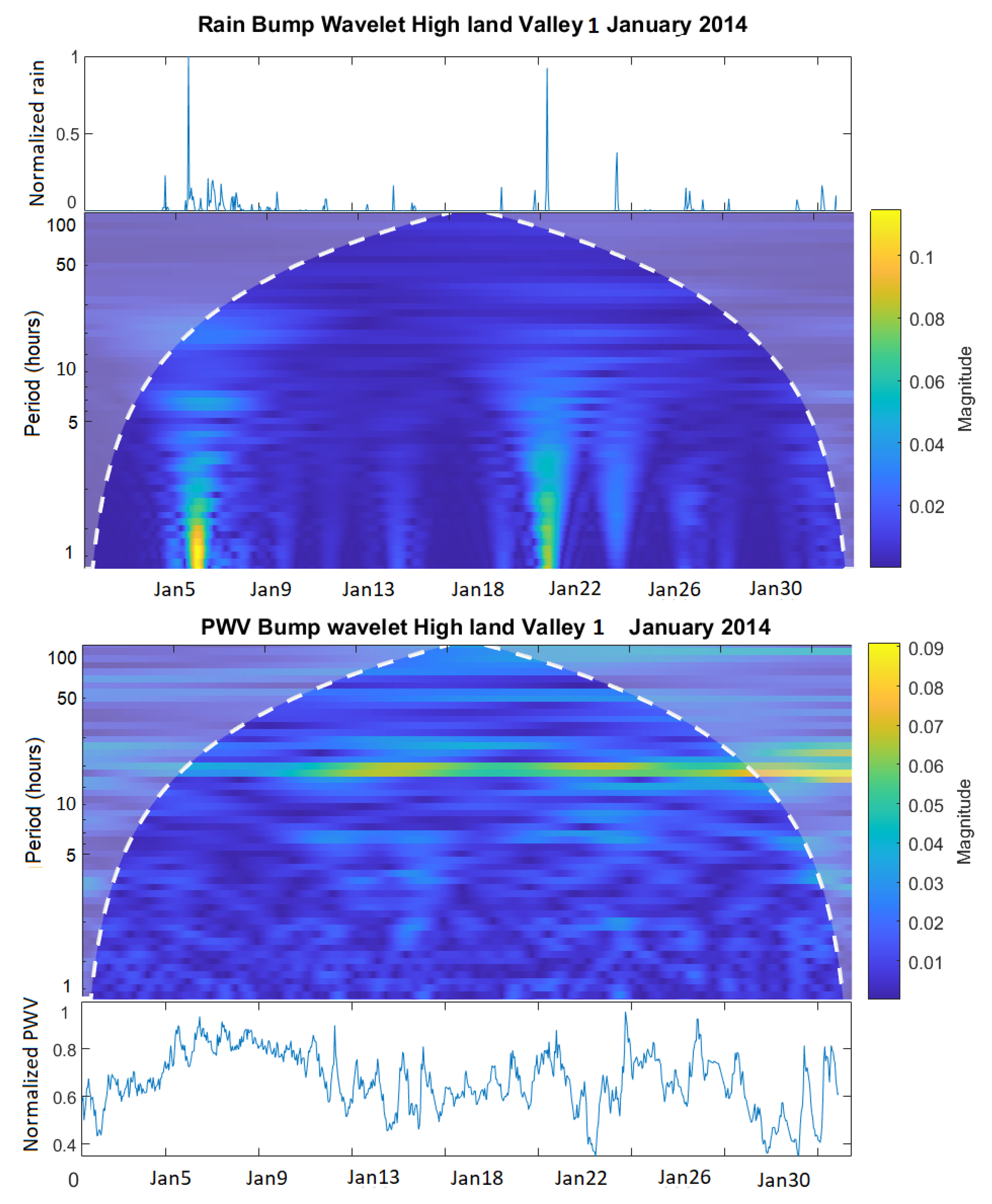
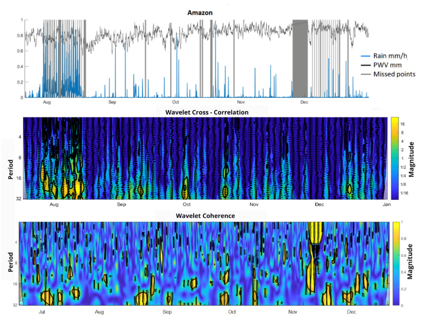
2.7.1. Continuous Wavelet Analysis: Transform, Coherence, and Cross-Spectrum

One of the objectives of this work is to find a correlation in the time-frequency domain between rain and PWV, that is, to determine the periods in which these two meteorological variables interact in a coordinated manner and in a localized period of time. The most appropriate tools for the effect are the wavelet coherence and cross-spectrum [37], as they provide the phase information between these signals. However, the continuous wavelet transform CWT is required for the calculation of any of them, and therefore becomes a previous step which enables the visualization of the harmonic content of the signals, that is, frequencies of interest that could provide additional or complementary information.
The computational analysis, data conditioning, simulations, and the plot of the results were performed with the aid of the Wavelets toolbox, Signal Processing toolbox, and Descriptive Statistics toolbox libraries (MathWorks, 2021), as well as the toolbox of Cross-wavelet and Wavelet Coherence by Grinsted [44].

Continuous Wavelet Transform

As a first step, the continuous wavelet or CWT transform was implemented to identify the harmonic behavior, if any, of both rain and water vapor. In essence, this transform decomposes a signal on a particular continuous wavelet wave.
A wavelet is a function ψ t of zero average,
ψ t d t = 0
This function ψ t is dilated with a scaling parameter s and translated in time with a parameter u :
ψ u , s t = 1 s ψ t u s
So, the wavelet transform W of a function f u , s , on the scale s and time position “ u ”, is calculated by correlating f with the wavelet signal [40].
W f u , s = f t 1 s ψ * t u s d t  
As it is observed, ψ t * , is the complex conjugate. W f u , s   can therefore measure the variations of spectral components just as the windowed Fourier transform or spectrogram does [45], but with a different time and frequency resolution. This is how through this CWT, very well-localized time and frequency packages can be determined but with the limitations of Heisenberg’s uncertainty principle [46]. For a mathematical explanation of this principle applied to time and frequency, see [40,45].
These packets that concentrate the energy of both time and frequency make up what is graphically known as a scalogram, which allows an identification at different scales of how the function f varies. If the “s” scale decreases, time support also decreases but the frequency range increases towards high frequencies. Similarly, if the “s” scale is dilated, the frequency range is located in the low-frequency range, but the support of the transform over time is enlarged.
The scalogram applied to the rain and PWV series, which are discrete functions in time (with hourly intervals in our case), would indicate in each case if they have harmonics or modes of interest throughout the year 2014. That is, the busiest intervals of repetitive events, whether they would be daily, weekly, monthly, or seasonal.
For our study, the scalograms were obtained by means of the bump-type analytical wavelet [43], given the fact that it narrows the variance of the CWT in frequency and thus allowing us to visualize with more finesse the periods of repetition of rain or PWV during certain time intervals of the series.

Bivariate Analysis with the Continuous Wavelet Transform

According to [47], if the CWT is applied to two time series, there is a geometric interpretation analogous to the covariance, which allows finding the common frequencies of these series, their location in time, and the common spectral power between these variables in two-dimensional graphs known as wavelet cross-correlation spectrum. It is important to mention that the covariance, unlike the correlation which is a value between −1 and +1, can take any value. Equation (6) determines the CWT of two time series   x t   and y t , after applying the individual wavelet transform on each of them, obtaining the functions W x u ,   s .   y W y u ,   s where u and   s are the time-location and frequency scale parameters, respectively, as it was noted in Equation (5). Therefore, the bivariate wavelet is
W x y u ,   s = S   W x u ,   s · W y u ,   s
Note that the asterisk represents the complex conjugate of the wavelet transform of the first series and S is a smoothing operator in time and frequency [43]. It can be clearly seen from this equation that the values to be operated on are complex. This is because the bivariate CWT uses an analytical (or complex) wavelet, thus obtaining the typical definition of the covariance of two complex random variables [48].
Then, we define the cross-wavelet power spectrum XWT in the following fashion:
XWT u ,   s = W x y u ,   s
the instantaneous lead phase, or relative phase angle between x t and y t , in the time-frequency space, is determined by calculating the complex argument of the bivariate transform. See [37].
θ   u ,   s = arg   W x y u ,   s
The libraries allow this phase to be calculated within the cross-spectrum plot through arrows, with the interval [−π, π]. An absolute value less than π/2 indicates that the two series tend to move in phase, having an ideal phase when the arrows point to the right horizontally. If the series tend to lag one another, the absolute value of the angle must be greater than π/2. If both signals oppose each other, or are in a complete out-of-phase, then the arrows are horizontal but left-oriented [49].
From Equations (7) and (8), it can be deducted that the XWT allows unveiling common high energy regions between the series, in our case rainfall and PWV, in addition to providing valuable information on the relationship of phase between these two. In other words, this is an important tool to be applied for the lead–lag analysis of the series of interest.
The libraries used the Morlet wavelet for the calculation of the XWT, since it provides an ideal balance in a location both in time and in frequency; this is because it has a complex exponential or carrier multiplied by a Gaussian or envelope window. This type of wavelet is also known as Gabor [40].
Note that a bivariate wavelet analysis benefits remarkably when evaluating the continuous wavelet coherence WTC, since the XWT cross-power spectrum is insufficient to analyze the correlations between a pair of processes in the time-frequency space, especially when the series has flat characteristics due to data loss or padding, such as in the case of the PWV. Their respective counterpart, on the other hand, presents pronounced peaks, as is the case of the rain. While the XWT reveals only the areas with the highest common concentrations of energy, the coherence reveals the local correlation of the two series in time and frequency throughout their extension and their localized phase behavior.
The continuous wavelet coherence WTC is obtained by normalizing the XWT, and it is appropriately known as the magnitude square coherence, and can be written as follows:
W T C x y u ,   s = S   W x u ,   s · W y u ,   s 2 S W x u ,   s 2 · S W y u ,   s 2
The smoothing operator “S” is equally present in the WTC in the same way as in Equation (6). This operator as explained in [39] performs a time smoothing followed by a frequency smoothing, although only time smoothing is possible according to [50]. Paying close attention to the WTC definition, it can be noticed that its structure is similar to the traditional method of obtaining the statistical correlation coefficient.
Therefore, the WTC is a complementary tool that serves to better analyze the behavior of rainfall and PWV, even in time and frequency segments that were not necessarily those detected by the XWT, but that could render useful information on the dynamics of these meteorological variables.

2.7.2. Simple Statistical Correlation as a Reference Parameter

As a precaution, the proposed wavelet tools cannot be applied blindly, but rather the data sets must be compared or tested with other models or mechanisms applicable to the process [44]. In our study, the control parameter for contrasting the results obtained by the XWT is the simple statistical cross-correlation [51] between the discrete vectors of the rainfall and PWV time series, since it would yield the lead of one signal over the other in units of time, where the maximum correlation coefficient is calculated. No previous treatment to the application of the cross-correlation was included because the stationarity of the specific rainfall events series is preserved [52].

2.7.3. Selection of Events of Interest by Their Statistical Significance Boundary

An event of interest is defined for this study as an intense rainfall occurrence, or in other words a sudden increase or peak in the hourly accumulated rain in the year 2014, which are selected for further analysis in order to determine its covariance with an associated PWV event preceding in time. Table 4 shows the max. rain occurrence, rain thershold and percentile of the most prominent events per station analyzed in this study.
The wavelet coherence WTC algorithm described in [37,53] was used to validate such events of interest because it allows the plotting of contours with a level of statistical significance of 5%. This is done by constructing a base background spectrum with white or red noise, on which the true spectrum of the wavelet coherence will be compared. These normalized-based spectrums, which are Chi-square distributed χ 2 2 , allow the construction of the statistical significance test. The premise, for a significance level α = 0.05 in our case, is that if the power of the WTC of the rainfall and PWV series is less than the normalized power of the wavelet coherence of two simulated base spectrum series, then the WTC wavelet power of the true signals is only generated due to random phenomena.
If instead the spectral power of the WTC of rainfall and PWV is greater than the spectral power obtained from operating the WTC of the series simulated with noise, the null hypothesis is discarded with a confidence level equal to (1 − α), 95% in our case, and it is inferred that the power of the WTC of the true signals is significantly larger than that generated by noise. The mathematical steps on how to obtain the statistical significance of the wavelet coherence WTC are very well explained in [54].
The WTC library [44] generates the surrogate noise series using data pairs which are the coefficients of the same lag-1 autoregressive model named AR(1). The WTC is calculated for each surrogate pair and with a Monte Carlo simulation approach the statistical significance level is estimated [50]. This library uses a default alpha α equal to 5% (0.05) for the significance test, in view of the fact that it provides an appropriate statistical balance to prevent Type 1 and Type 2 errors. By applying the wavelet coherence WTC, regions in time and scale (periods) can be identified with a confidence level above 95%. The time domain of these regions was used to locate the corresponding rainfall events of interest, in the time series, with the larger magnitudes or peaks.

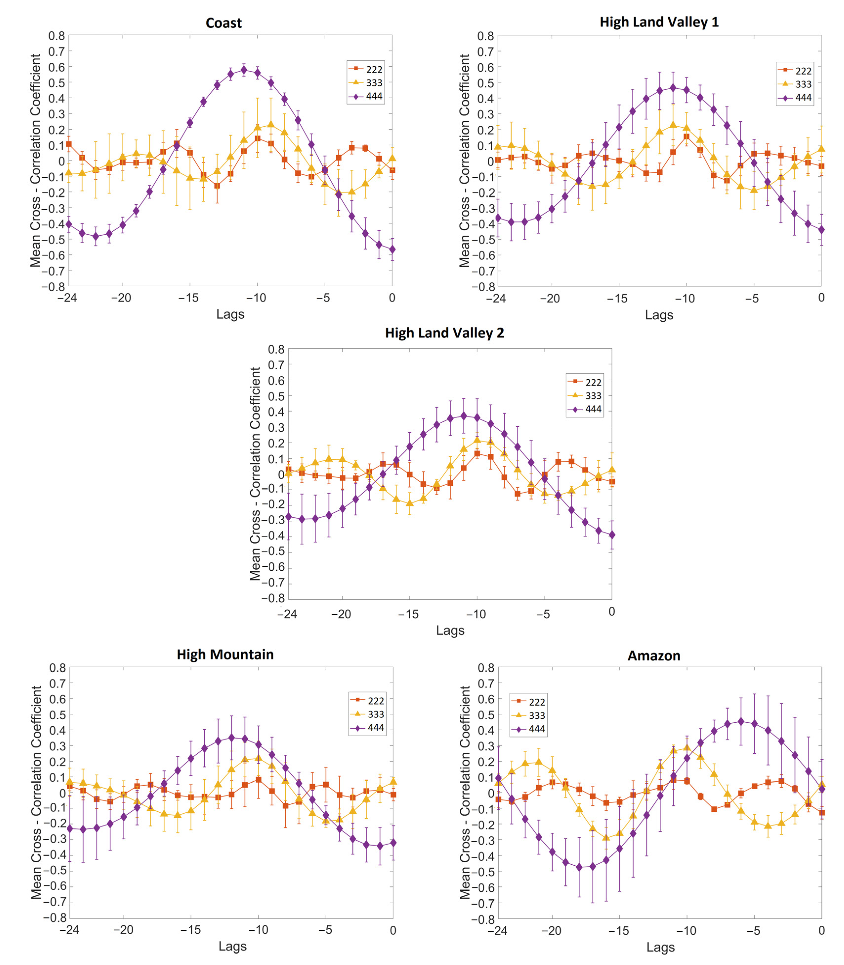
2.7.4. MRA Lead–Lag Analysis for the Events of Interest

Although the continuous wavelet spectrum plots obtained through XWT and WCT have important phase information that allows us to estimate the lead or lag that the rainfall presents with respect to the PWV, it is not without the compromise of accuracy since these plots can represent entire regions of energy spanning several days, even weeks or months along with a wide range of periods in the logarithmic scale. The phase accuracy can only be improved as far as the size of the analyzed energy atom can relate to the angle of orientation of a nearby arrow. It can be argued that the continuous bivariate analysis of the XWT and WCT is not meant to provide a quantity in particular, but the dynamic behavior of two signals for a particular time-frequency range or, better said, a region of significance.
Therefore, a multiresolution analysis or MRA method was used to obtain a quantifiable result of the phase content of the two series with hourly resolution. MRA refers to the method of decomposing a signal into sub-components or frequencies; there are many methods to perform signal decomposition and one of them is through discrete wavelets transform or DWT. There are several advantages of using the DWT over a CWT; for instance, faster computation and a wide choice of wavelets to choose from. A good reading for MRA fundamentals and examples can be found in [55].
The MRA decomposition of the rain and PWV series will produce different detail levels or one-dimensional scales (frequencies) for each one of them. The interesting fact is that these one-dimensional scales can be used in combination with a simple statistical cross-correlation approach to obtain the respective lag between a pair of rain and PWV scales. The larger the wavelet coefficients of the scale are, the more prominent the correlation coefficient would be and hence marking the lag between the different scales in hours.
Under this context, 20 events of interest were chosen per station which meet the following conditions: first, they have to correspond to the largest accumulated hourly rainfall data points that were detected per station; and second, that they shared with the PWV both coherence and the largest joint distribution energy over 95% confidence. Then, the final selection consisted of keeping mutually exclusive events that were not part of the same rain occurrence; in other words, that were at least 24 h apart in order to prevent overlapping with each other.
Other authors have used the cross-correlation of MRA scales of rain and PWV time series as in the case of [21]; however, with different time resolutions and possibly with different software tools. Note however that the results obtained in the present study are supported by a thorough continuous wavelet analysis (via cross-spectrum and coherence) and controlled by statistics in the time series as a way to make the lag selection process more objective and reliable.

2.8. Convection Analysis Using Satellite Images

Once the events of interest were obtained, the height of the clouds was analyzed one by one to identify deep convection through the GOES-13 satellite images in the infrared (IR) bands (10.2 to 11.2 μm), available every 30 min, both day and night, for Latin America from the Center Weather Forecast and Climate Studies (CPTEC) of the Government of Brazil available at http://satelite.cptec.inpe.br/acervo/goes16.formulario.logic?i=en, accessed on 21 March 2022 [56].
More than half of the incoming solar energy is absorbed by the planet’s surface is re-emitted as heat to space. As some of this energy passes up through the atmosphere clouds and atmospheric gases absorb a portion of this radiation. Then, the satellite IR channel senses radiation emitted by the earth’s surface, atmosphere, and cloud tops.
The IR images are colorized to bring out details in cloud patterns. In the colorized imagery used here clouds that have cloud-top temperatures colder than −80 °C are shown in pink and cloud-tops warmer than −30 °C are shown in orange. The colder the temperature, the taller the cloud-top height, and the relationship between temperature and cloud height is used to identify high, medium, or low clouds, with the more prominent heights being cumulonimbus clouds. Taller clouds correlate to more active weather such as stronger thunderstorms, and therefore a more convective activity.

2.9. Meteorological Anomalies of the Event’s Precipitation Threshold

The meteorological anomalies of atmospheric pressure, temperature, and wind speed were analyzed per station, in order to better visualize their behavior 24 h before and after the coherent rain events. Given the Gaussian nature of these variables, determined by a previous Shapiro–Wilk normality test, each anomaly is obtained by subtracting the meteorological variable minus its mean and is then divided by the standard deviation shown in Table 3. Both mean and standard deviation were calculated using the entire data set. Therefore, this anomaly is characterized by a dimensionless value in the interval [−3, 3]. These anomalies will complement the satellite images on the observed nature of rainfall, whether convective or stratiform, and its interactions with other local variables at each station.
The methodology and the steps of analysis applied to each station in order to obtain the relationship between rain and PWV are summarized in Figure 3. Note that atmospheric pressure was not available for Antisana (High Mountain station), therefore its derivation process is presented in Section 2.4.

3. Results

3.1. Meteorological Description of the Stations’ Location

The statistical analysis of every one of the available meteorological variables at each station for the year 2014, including the PWV and the missing data (NaN), is presented in Table 3. The stations are ordered from west to east, starting with the coast station (~45 m.a.s.l.), with a rain accumulation of 2640 mm/year, to the easternmost station located in the Amazon region (~553 m.a.s.l.), which is also the rainiest, with 3700 mm/year of accumulated precipitation. With increasing altitude, the annual accumulated rainfall decreases. The station with the highest altitude, located on Mount Antisana (4059 m.a.s.l.), records only precipitation of 415 mm/year.
In the same fashion, the variables of temperature and atmospheric pressure decrease with the altitude of the station, complying with Boyle’s Gas Law [57]. Regarding the behavior of the PWV, it can be seen that it decreases with altitude in most of the stations, with the exception of the high mountain station at Antisana which shows a precipitable water vapor as it is expressed in mm with a value of 21.52 ± 2.2 mm higher than the station at the Andes Valley in Quito, with 17.6 ± 1.7 mm. Despite the fact that the values of its rainfall are quite low; relative humidity, a magnitude which depends on both temperature and specific humidity, decreases at higher altitudes, except in high mountains where it increases due low temperatures. Wind registers the highest values in the high mountain station, with 4.56 ± 4.15 m/s, and a minimum in the Amazon station with 0.8 ± 0.6 m/s.
Figure 4 shows both the average hourly rainfall of the entire year 2014, including precipitation values ≥0, and the average hourly PWV per station. It can be seen that the diurnal cycle of these variables depends on the specific characteristics of the area, which produce rain with possible local origins. On the coast, land-sea breezes generated by the difference in heating between the sea and the coastal zone, which promotes convective rain at night [58]; steep-orography convective rain in the Andes valleys, which are usually present in the early morning and afternoon, and in the high mountain station, which favors rain during the day due to solar radiative forcing [59], especially in the high mountain region [60]; and a probable stratiform-convective rain in the Amazon region, in which the recorded precipitation does not adjust to a particular time or schedule.
Additionally, it can be noticed that the low variability of the hourly average PWV that present a slight increase during the hours when rain is less frequent.

3.2. Continuous and Discrete Wavelet Lead-Lag Analysis

The continuous wavelet analysis of the available rain and PWV data was performed for each station. Specifically, 12 months of data for the Andes Valley 1 and high mountain stations, and 6 months of data for the coast, Amazon region, and Andes Valley 2 stations.
As an example, Figure 5 shows a zoom-in of the wavelet plots of rain and PWV obtained from a bump-type analytic wavelet [43] for the Andes Valley 1 station for January 2014. It is evident how the presence of prominent rain events marks the magnitude of the wavelet plot, on which its lack of harmonic content can be seen except for the step-like frequency modes (periods) on 6 January and 22 January, whose intensity decreases as the period increases.
In contrast, when analyzing the CWT of the water vapor for the same time frame, a characteristic frequency of 24 h is present. In other words, throughout the time series, the influence of the diurnal cycle over the PWV, marked by the radiative forcing of the sun, is evident.
The wavelet analysis showed the non-periodical behavior of the rain for all stations, with a few localized exceptions where rain occurrences are well concentrated in a handful of days and whose noticeable periods do not exceed 6 or 8 h as shown above. Conversely, the wavelet plot of the PWV contains some acceptable harmonic content, enough to locate a 24 h year-round period for all stations (Appendix A, Figure A1) and well-localized minor sub-periods during certain days or weeks as in the case of the Amazon station, (Appendix A, Figure A1). These periods were extracted by using the Fourier Transform in the five stations.
Although the PWV and rainfall have harmonics in common, they are not necessarily in phase. On the contrary, as can be seen in Figure 4 and will be shown in subsequent analyses, these variables are in contra-phase (when it is maximum, the other is minimum).

3.2.1. Cross-Spectrum Wavelet XWT and Wavelet Coherence WTC Results

As shown in Figure 5, it is hard for a simple continuous wavelet to transform to point out any possible link between the series of rain and PWV. Therefore, a continuous cross-spectrum calculation of the wavelets transforms or XWT is performed as well as their wavelet transform coherence WTC as explained in Equation (7) and Equation (9), in order to determine the time-frequency areas where both rain and PWV show a common energy activity and are covariant at the same time with a level of confidence of at least 95%.
Appendix B (Figure A2) shows the XWT and WTC performed for each station for all data available in 2014. However, note that the study focuses on the plot areas where coherence and significant cross-spectrum shared the same time and frequency, so a zoom-in of such areas was necessary to determine the events of interest with a better resolution, as shown in Figure 6. The thick contour around the areas of maximum energy is referred to as the boundary of statistical significance of 5%.
It was found that areas with the largest power of XWT are due to the presence of important rain events. The larger the rain event, the stronger the power of the magnitude of XWT. This is because the XWT provides us with a measure of the power distribution of two signals. Hence, it is important to obtain the WTC coherence to determine which mutual events of rain and PWV have a true joint variability, as it was observed that there was no coherence with the PWV for all intense rainfall events, at least with a statistical confidence level greater than 95%.
The XWT and WTC are plotted to show periods of repetition (frequencies) of up to 32 h, with the aim of finding sub-diurnal relationships. For example, Figure 6 shows that the XWT has important periods well localized between 6 January and 9 January and also between 22 January and 26 January, being the more important ones, the periods ranging from the hours 16 to 32 in the first case, and periods centered around the hours 12 and 24 in the latter one. On the other hand, the WTC shows many areas where it can be said that the rain and PWV are covariant, the larger ones being the regions from 5 January to 9 January, 12 January to 18 January, and 26 January to 30 January, but did not consider the intense event of Jan. 22th. These regions comprise periods ranging mainly from hours 16 to 32.
The phase content of the rain and PWV can be determined from the direction of the arrows in the plot. It can be noted in Figure 6 that the only section where there is coherence and high energy activity, as matched with the above rainfall time series, corresponds to the intense event of 6 January. The arrows in this case are pointing to the left, indicating a complete out-of-phase scenario, where the PWV precedes the rain series in a half cycle as explained in Equation (8). The periods of peak energy are localized between hours 20 and 24 as seen from the XWT plot, thus the lag for the 6 January event can be calculated between hours 10 and 12, respectively.
It is interesting to note that approximately 12 h of lag will be common in all stations (Appendix B, Figure A2); this fact is also obtained from Figure 4, although less evidently, where high PWV values occur at the hourly level when the rain decreases, as if it were a continuous daily process where the PWV builds up, to later release itself previous to a rainfall event at particular hours during the day.
Table 4 shows the number of selected intense events with XWT and WTC with a confidence level above 95% between PWV and rainfall, among the largest selected independent rainfall events. Note that not all the intense events show XWT and WTC, i.e., not all the intense events were preceded by a PWV peak. In the same way, the rainfall threshold values are presented with their respective percentile, in addition to the maximum values and the median (50th percentile).
Additionally, Table 4 shows the climatic difference among the regions of study, not only for the quantity of accumulated rain found at each station of Table 3, but for their observed dissimilar maximum values and hourly intensity thresholds of rain (marked by the minimum rainfall value of the selected events of interest). It should be noted that all the stations register an identical minimum value of hourly accumulated precipitation equal to 0.1 mm/h, marked by the precision of the pluviometers. Note also the rapid decrease in the values of rainfall intensities since this value is close to the 50th percentile in all cases.
The coastal station is the only one where all the maximum accumulated rainfall intensity events show coherence and peak energy above the 95% confidence level boundary with the PWV, and therefore were preceded by a PWV peak. This fact may be due to the sea breeze phenomenon which is much more homogeneous and with less variability [58] than the events that occur in the steep orography of the Andes or in the Amazon region, where various climatic factors produce intense precipitation [61]. For other stations (Appendix B, Figure A2), these events are intercalated between the maximum values, although the largest event of the year always presents a correlation and a peak energy with the PWV.

3.2.2. Lead–Lag Discrete Wavelet and Convection Analysis for the Events of Interest

In order to define a more precise magnitude of the lag between the PWV and intense rain peaks, a discrete wavelet analysis was performed and a data set with as many samples as possible around the events of interest was constructed. Given the constraints that each event had to abide by, some event’s data sets were as short as 9 days (the truncated ones that occurred when intense events occurred close to each other) and as long as 30 days. This was performed for each station to assure a more reliable lead–lag calculation given the hourly resolution of the samples.
Once the data sets were obtained, a wavelet cross-correlation D-WCC calculation by using a Daubechies wavelet of order 20, was implemented. This wavelet was selected due to its ability to be implemented with a large number of vanishing moments, which are useful when analyzing complex signals, as well as due to its widely available information and implementation in MRA [41].
The Wavelet Toolbox [43] was very useful to decompose each of the data sets of interest for rain and PWV. Up to five different levels of detail can be seen by selecting the db10 (Order 20 Daubechies wavelet). These levels of detail are the plot of the wavelet coefficients obtained by performing the discrete wavelet transform in dyadic scales.
The selection of the levels of detail of rain and PWV was the most taunting one, since the amplitude of these coefficients has a direct impact on the final wavelet cross-correlation calculation and therefore the lag. Nonetheless, a trade-off was necessary in some cases given the constraints of the algorithm used to calculate the wavelet cross-correlation, which required same-size datasets to be operated. That said, the results were obtained from the same level coefficients for the rain and PWV.
The most representative levels of detail, from two to four, were obtained from all data sets of rain and PWV related to each event of interest and cross-correlated with the purpose of calculating their correlation coefficients and corresponding lag. This treatment was performed for all events of interest and per station. Figure 7 shows the average D-WCC of the levels per station with their respective standard deviation. Note that the D-WCC yields a matrix of cross-correlation coefficients obtained from the different levels of decomposition of the discrete db10 wavelets of each series. For that reason, a Level (x, y, z) indicates the cross-correlation of all levels of decomposition, x for the rain and y for the PWV, from which the level z is selected for analysis or plotting.
Level 444 has been the one with the highest correlation for all stations in this study. This means that the db10 discrete wavelet transform of the rain and PWV performed down to four levels of decomposition, yielded the highest cross-correlation coefficients at the fourth level.
The average correlation at level 444 in the coast station was not only the highest, but also the least dispersed, showing the most homogeneous behavior of all five stations, and providing the highest average lag at 11 h. Levels 222 and 333 presented higher dispersion and a smaller correlation coefficient than level 444, with a lag of 10 h and 9 h, respectively.
Similarly, at the Andes Valley 1 station, the average lag was located very close to each other for the analyzed levels of decomposition. A lag of 11, 11, and 9 h were obtained for levels 444, 333, and 222, respectively. In the case of Andes Valley 2, a lag of 11, 10, and 10 h were obtained at the same levels. In the High Mountain station, a lag of 12, 10, and 10 h were obtained for the same levels. These results change when analyzing the Amazon station, where the largest lag corresponded to 6, 10, and 3 h for levels 444, 333, and 222, respectively.
Table 5 collects the individual analysis of the studied events, indicating the date and time of the event of interest, the magnitude of the recorded rainfall, as well as the level of decomposition that provided the greatest correlation. Note also that the value of the simple statistical correlation of the time series is included as a control parameter, to corroborate the value of the lag calculated with the discrete wavelet transform. The sign of the lag achieved confirms that the peak that precedes the rain is from the PWV. Finally, a convection analysis achieved from satellite images complements Table 5.
With respect to the coast station, it presents a well-localized lag at 11 h with most rain events occurring at night, which corresponds to the diurnal cycle presented in Figure 4. The major rain events are not only shared with the PWV coherence and peak energies, but also convection. It could be inferred that the sea breeze influences the dynamics between rainfall and PWV, not only because it allows uniformity in the lag but also because it could be decisive in the presence of convection on the coast.
In the case of the Andes Valley 1 station, the largest events are recorded in the afternoon and early morning, which corresponds again to its diurnal cycle. While in Andes Valley 2 station, the largest events happen in the afternoon, with exception of one event recorded at dawn. Additionally, the high mountain station presents its events only during the day. In these three Andean stations, coherence between PWV and rain does not always occur, as shown in Table 5, i.e., the PWV peak does not always precede intense rainfall. Furthermore, it can be said then that convection is present in almost all events at these stations. Therefore, the relationship between the PWV peaks and rainfall is more complex than at the coast one station, and PWV is not always the only precursor for the generation of an intense rainfall event. Additionally, the orography of the Andes region plays an important role in stimulating this convective process.
The Amazon station has the most intense hourly accumulated rain events of the studied series, and in the Andean case not all intense rain events share coherence and peak energy with the PWV. Furthermore, in contrast with the rest of the stations, there is not a regular time during the day when rain occurs. The PWV periods found in the wavelet analysis are scattered and should be further analyzed. In the cases where there was coherence between the series, the selected events have shorter lags, which range from 5 to 10 h at most. The convection is minimal since the generation of high convective clouds is probably not required in order to achieve intense precipitation; it has already been discussed that the rain in this station may have a stratiform origin, produced by the advection of humidity masses transported through the Amazon jungle by the trade winds, differing as such from the other stations.

3.3. Analysis of Convective Clouds Using Satellite Images

The convection analysis presented in Table 5 has been obtained from the images in Figure 8. Note that convective events are represented by pink, blue, turquoise, yellow, and orange spots representing cloud top heights from −80 °C to −30 °C. The highest corresponds to tall vertical formations related to cumulonimbus clouds, and hence to convective rain. Only the Amazon station (Tena) shows one event of convective rain, and the rest of the occurrences correspond to low- or medium-height clouds. The analysis of the presence of high clouds tops and medium clouds, with lag evaluation, is presented in Table 5.

3.4. Analysis of Meteorological Anomalies

Figure 9 shows the average of the meteorological anomalies, 24 h before and after the selected rain events, which were centered at 0 h. These anomalies were calculated as explained in Section 2.9, using the data presented in Table 3. The atmospheric pressure anomalies (Figure 9a), show different behavior between the stations of the Andes, high mountain, and coast vs. the behavior of the Amazon station. In the first ones, a decrease in pressure is appreciated before the rainy event, which could indicate local convection caused either by the orography of the Andes, or due to the phenomenon of the sea breeze on the coast. However, in the Amazon station, this decrease in pressure is not appreciable. A phenomenon that may point to the stratiform nature of the rains in the Amazon region is caused by advective movements of moisture transport [61], in accordance with the preceding results.
In Figure 9b, a fairly regular behavior is observed with regard to wind speed, except at the coast station, where a marked increase in wind speed is seen in the presence of a rainfall event, possibly due to the effect of the sea breeze which could generate considerable winds [58]. Finally, when analyzing Figure 9c, it can be noted a generalized behavior is marked by a decrease in temperature as a result of the rain event, a phenomenon explained by the subsequent evaporation of precipitation and, therefore, absorption of latent heat from the surroundings [57,58,59,60].

4. Discussion

Considering the results, it can be noted the difference between the relationship between the PWV and the intense rainfall for the different climatic zones of Ecuador. The most homogeneous relationship is the one found at the coast station, showing the greatest predictive potential of the PWV peaks before an intense rain event. In the Andes, these relationships are less common and despite the fact that they exist, they also obey other dynamics that must be considered for the generation of intense rain. Similarly, in the case of the Amazon region, correlations between PWV and intense rainfall events do exist, but they are due to different climatic factors than in the previous cases.
The PWV and rainfall series around the selected intense events for the coast station presented both correlation and coherence. The dispersion of the lags encountered for the PWV preceding the intense rain was minimal at the highest correlation coefficient located at 11 h. Additionally, convection was found in almost all those events. It can be said that the phenomenon of sea breeze, the main driver of precipitation events on the coast, is dynamically the most uniform aspect of the studied areas.
In the Andes stations, correlation and coherence were found in a scattered way in a number of events chosen. A total value of 64.3% of the sampled events showed correlation and coherence for the case of Andes Valley 1. This could be indicative of the presence of other dynamic factors such as the topography of the area, leaving the relationship between PWV and rainfall as an important driver of intense rain but not an essential one. The selected events of interest which presented coherence with the PWV generated a lag similar to the coast, being close to 11 h. This is also similar to Andes Valley 2, where 53% of the events presented coherence and the most significant lag was at 11 h. The high mountain station, with 77% of events sharing coherence with the PWV, showed the most dispersed lag found at 12, 10, and 6 h.
The fact that the most common lag is found at 11 h for both the coast and Andes regions may have to do with the presence of more probable hours for precipitation (see Figure 4). This influence of the diurnal cycle favors the PWV recharge before the occurrence of an intense rainfall event, and even if it is not an intense rain, there are preferable hours for PWV to recharge in order to discharge in the rainfall most probable occurrence hours, in accordance with [62]. The effect of the diurnal cycle is ubiquitous for PWV at the coast and in the Andes regions as shown in Figure A1 and Figure 5, with characteristic periods of 12 h and 24 h reported [63]. Furthermore, it should be noted from the cross-spectrum plot XWT that the PWV and rainfall have the same region of covariance centered at the 24 h period.
Unlike the other regions, the Amazon station shows different behavior for the PWV and rain. There are no preferred hours for precipitation (Figure 4) and the 24 h period is not unique, with other major periods appearing for PWV (Figure A1). Furthermore, the winds are minimal (Table 3), in addition to the fact that local convection is not necessary for the formation of intense rain. The main cause of rain in this region could be the advective transfer of moist air masses by trade winds [61,64,65] and its subsequent orographic forcing when touching the eastern mountain range of Ecuador (see Figure 1). This transport is responsible for both the generation of water vapor peaks and rain, but due to the greater frequency of rainy events, this lag between PWV peaks and rain is shorter: 6, 10, and 3 h for the wavelet levels analyzed, and not necessarily due to the diurnal cycle. These results are in agreement with other studies in the region [22]. Satellite images and the study of meteorological anomalies (Figure 9) show that there is no evidence of a significant decrease in atmospheric pressure before the rainfall event, which reinforces the fact that stratiform rainfall is preponderant at the Amazonian station.

5. Conclusions

This study shows the potential of harmonic analysis tools to characterize the relationship between the PWV and rainfall, with the aim of possibly anticipating the occurrence of an intense rainfall event in different climatic zones. The area that showed the most consistent relationships between these variables was the coast, where all rainfall events were preceded by peaks in water vapor within 95% of confidence. This fact points to the importance of the PWV dynamics for the occurrence of intense rain events, in accordance with previous investigations carried out in other coastal areas such as Portugal [19], Italia [10], and China [17,18]. Nevertheless, the reported lag is different, which may be due not only to the choice of short windows in the study of this lag, but also to other dynamic factors of each locality that must be considered.
In contrast, in the Andes, this relationship loses consistency, since only 53% to 77% of intense rainfall events were preceded by water vapor peaks. These types of studies in high-altitude areas have been little reported [62] and show the importance not only of the appearance of PWV peaks, but of other factors such as the topography in the occurrence of intense rainfall events. Likewise, in the Amazon region, where 66.7% of rain events preceded by PWV peaks were reported, the importance of other atmospheric phenomena is also appreciated, such as the advective transport of moisture carried by the trade winds from the Amazon. The reported lag was also found in previous studies [22].
This study identified two types of lag, the first around 11 h, and found both on the coast and in the Andean areas, which had rainfall characterized by connectivity and determined rainfall occurrence times. Smaller lag (around 6 h) was recorded in the Amazon area, which coincides with previous research [21,22]. In this region, no preferred times for the occurrence of rain were identified, and most of the intense events were stratiform. It is possible that one of these factors or both influences the duration of the reported lag.
Therefore, the present study is an attempt to understand the relationships between PWV and rainfall in regions that have been identified for this purpose as relevant and with different climatology. Likewise, the integration of not only high-resolution regional models but also re-analyses of atmospheric circulation would be of great help to interpret other physical connections deemed important and necessary. Further progress would be the improvement of the tropospheric models through the adequate assimilation of GNSS-PWV data. All these factors will improve not only the better prediction of severe intense rain events, but also their comprehension in a complementary way to the traditional ones.
It is also important to highlight the contrast between the different harmonic analysis tools used in this study. Despite the featureless results provided by the spectrogram of a single variable wavelet analysis, when combined with statistics in a bivariate approach to obtain the cross-spectrum and coherence scalograms, the results are more significant. Time-frequency regions that would go otherwise unnoticed are now evident with a level of statistical significance including the phase content (lead or lag) between rain and PWV. The discrete wavelet analysis using Daubechies 20 was performed to validate the results of the cross-spectrum scalogram and to determine a measurable quantity that could be compared to the traditional statistical correlation method used as a control parameter.
Further research with data sets containing longer periods of time, perhaps years if not decades, and sampled to better temporal resolutions, are necessary in order to increase the understanding of the relationship between rain and PWV, improve the harmonic content of the results, and accuracy of the lag in the aforementioned geographical areas. Although this is not always possible in stations located in remote or hard-to-access areas, refurbishing, maintaining, and expanding the current meteorological network will allow better data collection and data logging in the long term,

Author Contributions

M.V., T.C., L.C., L.A.E., A.W. and S.S.-V. contributed to the conception and design of the methodology of the study. S.S.-V. and A.W. made computations, S.S.-V. and D.C.-M. organized the database and performed the statistical analysis, S.S.-V. and L.A.E. wrote the original draft preparation and conducted the formal analysis of the results presented in the study. Supervision, validation, review, and editing were performed by M.V., T.C., L.C., L.A.E. and A.W. All authors have read and agreed to the published version of the manuscript.

Funding

This research was funded by Universidad Politécnica Salesiana doctoral scholarships and the IRD and EPN for the LMI GREATICE grant.

Data Availability Statement

Rinex GNSS data is available in the database of UNAVCO https://www.unavco.org/data/gps-gnss/gps-gnss.html, accessed on 21 March 2019. Satellite imagery of Latin America is available from the Center Weather Forecast and Climate Studies (CPTEC) of the Government of Brazil, available at http://satelite.cptec.inpe.br/acervo/goes16.formulario.logic?i=en, accessed on 21 March 2019 [56].

Acknowledgments

The authors thank INAMHI, IRD, and REMMAQ for the provided data. We also thank Luis Maisincho and Jean Carlos Ruiz for their contributions and valuable discussions for this research. Finally, our acknowledgment to Luis Muñoz and Jéssica Guamán for their collaboration with Figure 1 and Appendix A (Figure A1).

Conflicts of Interest

The authors declare no conflict of interest that may be perceived as inappropriately influencing the representation or interpretation of reported research results.

Appendix A

Characteristic periods of (a) PWV. Note the marked period of 24 h and the secondary one of 12. In the Amazon region, the spectral density is lower and there are two more characteristic periods of 8 and 16 h (b) rain. Note the lower spectral density in comparison with PWV, and the characteristic period of around 24 h.
Figure A1. Characteristic periods of (a) PWV. Note the marked period of 24 h and the secondary one of 12. In the Amazon region, the spectral density is lower and there are two more characteristic periods of 8 and 16 h (b) rain. Note the lower spectral density in comparison with PWV, and the characteristic period of around 24 h.
Atmosphere 13 01809 g0a1

Appendix B

Wavelet Cross-Spectrum (XWT) and Wavelet Transform Coherence (WTC) of the stations for the year 2014 for the Coast, Andes Valley 1, Andes Valley 2, High Mountain and Amazon.
Figure A2. Wavelet Cross-Spectrum (XWT) and Wavelet Transform Coherence (WTC) of the stations for the year 2014 for the Coast, Andes Valley 1, Andes Valley 2, High Mountain and Amazon.
Atmosphere 13 01809 g0a2aAtmosphere 13 01809 g0a2bAtmosphere 13 01809 g0a2c

References

  1. Businger, S.; Chiswell, S.R.; Bevis, M.; Duan, J.; Anthes, R.A.; Rocken, C.; Ware, R.H.; Exner, M.; VanHove, T.; Solheim, F.S. The Promise of GPS in Atmospheric Monitoring. Bull. Am. Meteorol. Soc. 1996, 77, 5–18. [Google Scholar] [CrossRef]
  2. Bonafoni, S.; Biondi, R.; Brenot, H.; Anthes, R. Radio Occultation and Ground-Based GNSS Products for Observing, Understanding and Predicting Extreme Events: A Review. Atmos. Res. 2019, 230, 104624. [Google Scholar] [CrossRef]
  3. Bevis, M.; Businger, S.; Herring, T.A.; Rocken, C.; Anthes, R.A.; Ware, R.H. GPS Meteorology: Remote Sensing of Atmospheric Water Vapor Using the Global Positioning System. J. Geophys. Res. 1992, 97, 787–801. [Google Scholar] [CrossRef]
  4. Bevis, M.; Businger, S.; Chiswell, S.; Herring, T.A.; Anthes, R.A.; Rocken, C.; Ware, R.H. GPS Meteorology: Mapping Zenith Wet Delays onto Precipitable Water. J. Appl. Meteorol. 1994, 33, 379–386. [Google Scholar] [CrossRef]
  5. Yeh, T.K.; Hong, J.S.; Wang, C.S.; Chen, C.H.; Chen, K.H.; Fong, C.T. Determining the Precipitable Water Vapor with Ground-Based GPS and Comparing Its Yearly Variation to Rainfall over Taiwan. Adv. Space Res. 2016, 57, 2496–2507. [Google Scholar] [CrossRef]
  6. Sguerso, D.; Labbouz, L.; Walpersdorf, A. 14 Years of GPS Tropospheric Delays in the French–Italian Border Region: Comparisons and First Application in a Case Study. Appl. Geomat. 2016, 8, 13–25. [Google Scholar] [CrossRef]
  7. Walpersdorf, A.; Bouin, M.; Bock, O.; Doerflinger, E. Assessment of GPS Data for Meteorological Applications over Africa: Study of Error Sources and Analysis of Positioning Accuracy. J. Atmos. Sol. Terr. Phys. 2007, 69, 1312–1330. [Google Scholar] [CrossRef]
  8. Brenot, H.; Walpersdorf, A.; Reverdy, M.; van Baelen, J.; Ducrocq, V.; Champollion, C.; Masson, F.; van Baelen, J.; Doerflinger, E.; Collard, P.; et al. A GPS Network for Tropospheric Tomography in the Framework of the Mediterranean Hydrometeorological Observatory Cévennes-Vivarais (Southeastern France). Atmos. Meas. Tech. 2014, 7, 553–578. [Google Scholar] [CrossRef] [Green Version]
  9. Padullés, R.; Kuo, Y.-H.; Neelin, J.D.; Turk, F.J.; Ao, C.O.; De la Torre Juárez, M. Global Tropical Precipitation Relationships to Free Tropospheric Water Vapor Using Radio Occultations. J. Atmos. Sci. 2022, 79, 1585–1600. [Google Scholar] [CrossRef]
  10. Bonafoni, S.; Biondi, R. The Usefulness of the Global Navigation Satellite Systems (GNSS) in the Analysis of Precipitation Events. Atmos. Res. 2016, 167, 15–23. [Google Scholar] [CrossRef]
  11. Shoji, Y.; Kunii, M.; Saito, K. Assimilation of Nationwide and Global GPS PWV Data for a Heavy Rain Event on 28 July 2008 in Hokuriku and Kinki, Japan. Sola 2009, 5, 45–48. [Google Scholar] [CrossRef] [Green Version]
  12. Risanto, C.B.; Castro, C.L.; Arellano, A.F., Jr.; Moker, J.M., Jr.; Adams, D.K. The Impact of Assimilating GPS Precipitable Water Vapor in Convective-Permitting WRF-ARW on North American Monsoon Precipitation Forecasts over Northwest Mexico. Mon. Weather Rev. 2021, 149, 3013–3035. [Google Scholar] [CrossRef]
  13. Li, H.; Wang, X.; Wu, S.; Zhang, K.; Chen, X.; Qiu, C.; Zhang, S.; Zhang, J.; Xie, M.; Li, L. Development of an Improved Model for Prediction of Short-Term Heavy Precipitation Based on Gnss-Derived Pwv. Remote Sens. 2020, 12, 4101. [Google Scholar] [CrossRef]
  14. Li, L.; Zhang, K.; Wu, S.; Li, H.; Wang, X.; Hu, A.; Li, W.; Fu, E.; Zhang, M.; Shen, Z. An Improved Method for Rainfall Forecast Based on GNSS-PWV. Remote Sens. 2022, 14, 4280. [Google Scholar] [CrossRef]
  15. Labbouz, L.; van Baelen, J.; Duroure, C. Investigation of the Links between Water Vapor Field Evolution and Rain Rate Based on 5 Years of Measurements at a Midlatitude Site. Geophys. Res. Lett. 2015, 42, 9538–9545. [Google Scholar] [CrossRef]
  16. Pendergrass, A.G. What Precipitation Is Extreme? Science 2018, 360, 1072–1073. [Google Scholar] [CrossRef]
  17. Yao, Y.; Shan, L.; Zhao, Q. Establishing a Method of Short-Term Rainfall Forecasting Based on GNSS-Derived PWV and Its Application. Sci. Rep. 2017, 7, 12465. [Google Scholar] [CrossRef] [Green Version]
  18. Zhao, Q.; Ma, X.; Yao, Y. Preliminary Result of Capturing the Signature of Heavy Rainfall Events Using the 2-d-/4-d Water Vapour Information Derived from GNSS Measurement in Hong Kong. Adv. Space Res. 2020, 66, 1537–1550. [Google Scholar] [CrossRef]
  19. Benevides, P.; Catalao, J.; Miranda, P.M.A. On the Inclusion of GPS Precipitable Water Vapour in the Nowcasting of Rainfall. Nat. Hazards Earth Syst. Sci. Discuss. 2015, 3, 3861–3895. [Google Scholar] [CrossRef] [Green Version]
  20. Benevides, P.; Catalao, J.; Nico, G. Neural Network Approach to Forecast Hourly Intense Rainfall Using GNSS Precipitable Water Vapor and Meteorological Sensors. Remote Sens. 2019, 11, 917. [Google Scholar] [CrossRef]
  21. Sapucci, L.F.; Machado, L.A.T.; de Souza, E.M.; Campos, T.B. Global Positioning System Precipitable Water Vapour (GPS-PWV) Jumps before Intense Rain Events: A Potential Application to Nowcasting. Meteorol. Appl. 2019, 26, 49–63. [Google Scholar] [CrossRef] [Green Version]
  22. Adams, D.K.; Gutman, S.I.; Holub, K.L.; Pereira, D.S. GNSS Observations of Deep Convective Time Scales in the Amazon. Geophys. Res. Lett. 2013, 40, 2818–2823. [Google Scholar] [CrossRef]
  23. Calori, A.; Santos, J.R.; Blanco, M.; Pessano, H.; Llamedo, P.; Alexander, P.; de la Torre, A. Ground-Based GNSS Network and Integrated Water Vapor Mapping during the Development of Severe Storms at the Cuyo Region (Argentina). Atmos. Res. 2016, 176, 267–275. [Google Scholar] [CrossRef]
  24. Ayala, M.F.; Carrera-Villacrés, D.; Tierra, A. Relación Espacio-Temporal Entre Estaciones Utilizadas Para El Relleno de Datos de Precipitación En Chone, Ecuador. Rev. Geográfica Venez. 2018, 59, 298–313. [Google Scholar]
  25. Romero, R.; Pilapanta, C.; Porras, L.; Tierra, A. Prediction of Precipitable Water Vapor With a Neural Network From the Ecuadorian Gnss and Meteorological Data. Rev. Geoespacial 2019, 15, 1. [Google Scholar] [CrossRef]
  26. Herring, T.A.; King, R.W.; McClusky, S.C. Introduction to GAMIT/GLOBK; Massachusetts Institute of Technology: Cambridge, MA, USA, 2018; pp. 1–16. [Google Scholar]
  27. Wagnon, P.; Lafaysse, M.; Lejeune, Y.; Maisincho, L.; Rojas, M.; Chazarin, J.P. Understanding and Modeling the Physical Processes That Govern the Melting of Snow Cover in a Tropical Mountain Environment in Ecuador. J. Geophys. Res. Atmos. 2009, 114, 1–14. [Google Scholar] [CrossRef]
  28. Brenot, H.; Ducrocq, V.; Walpersdorf, A.; Champollion, C.; Caumont, O. GPS Zenith Delay Sensitivity Evaluated from High-Resolution Numerical Weather Prediction Simulations of the 8-9 September 2002 Flash Flood over Southeastern France. J. Geophys. Res. 2006, 111, 15105. [Google Scholar] [CrossRef] [Green Version]
  29. Climate World. Programme Guidelines on the Quality Control of Surface Climatological Data; World Meteorological Organization: Geneva, Switzerland, 1986. [Google Scholar]
  30. Lanzante, J.R. Resistant, Robust and Non-Parametric Techniques for the Analysis of Climate Data: Theory and Examples, Including Applications to Historical Radiosonde Station Data. Int. J. Climatol. 1996, 16, 1197–1226. [Google Scholar] [CrossRef]
  31. Cho, H.-K.; Bowman, K.P.; North, G.R. A Comparison of Gamma and Lognormal Distributions for Characterizing Satellite Rain Rates from the Tropical Rainfall Measuring Mission. J. Appl. Meteorol. 2004, 43, 1586–1597. [Google Scholar] [CrossRef]
  32. Serrano-Vincenti, S.; Condom, T.; Campozano, L.; Guamán, J.; Villacís, M. An Empirical Model for Rainfall Maximums Conditioned to Tropospheric Water Vapor Over the Eastern Pacific Ocean. Front. Earth Sci. 2020, 8, 198. [Google Scholar] [CrossRef]
  33. Lewis, E.; Quinn, N.; Blenkinsop, S.; Fowler, H.J.; Freer, J.; Tanguy, M.; Hitt, O.; Coxon, G.; Bates, P.; Woods, R. A Rule Based Quality Control Method for Hourly Rainfall Data and a 1 km Resolution Gridded Hourly Rainfall Dataset for Great Britain: CEH-GEAR1hr. J. Hydrol. 2018, 564, 930–943. [Google Scholar] [CrossRef]
  34. Garratt, R.J. The Atmospheric Boundary Layer; Press, C., Ed.; Elsevier: Amsterdam, The Netherlands, 1992. [Google Scholar]
  35. Fernández, L.I.; Meza, A.M.; Natali, M.P. Determinación Del Contenido de Vapor de Agua Precipitable (PWV) a Partir de Mediciones GPS: Primeros Resultados En Argentina. Geoacta 2009, 34, 35–57. [Google Scholar]
  36. Emardson, T.; Derks, H. On the Relation Between the Wet Delay and the Integrated Precipitable Water Vapour in the European Atmosphere. Meteorol. Appl. 1992, 7, 61–68. [Google Scholar] [CrossRef]
  37. Grinsted, A.; Moore, J.C.; Jevrejeva, S. Application of the Cross Wavelet Transform and Wavelet Coherence to Geophysical Time Series. Nonlinear Process. Geophys. 2004, 11, 561–566. [Google Scholar] [CrossRef]
  38. Yang, M.; Yao, T.; Gou, X.; Wang, H.; Neumann, T. Wavelet Analysis Reveals Periodic Oscillations in a 1700 Year Ice-Core Record from Guliya. Ann. Glaciol. 2006, 43, 132–136. [Google Scholar] [CrossRef] [Green Version]
  39. Torrence, C.; Compo, G.P. A Practical Guide to Wavelet Analysis. Bull. Am. Meteorol. Soc. 1998, 79, 61–78. [Google Scholar] [CrossRef]
  40. Mallat, S. A Wavelet Tour of Signal Processing; Elsevier: Amsterdam, The Netherlands, 1999; ISBN 9780080520834. [Google Scholar]
  41. Daubechies, I. Ten Lectures on Wavelets; SIAM: Philadelphia, PA, USA, 1992; ISBN 978-1-61197-010-4. [Google Scholar]
  42. Chui, C.K. An Introduction to Wavelets; Academic Press: New York, NY, USA, 1992; ISBN 9781483282862. [Google Scholar]
  43. Mathworks Choose a Wavelet 2021 Homepage. Available online: https://la.mathworks.com/help/wavelet/gs/choose-a-wavelet.html (accessed on 20 July 2022).
  44. Grinsted, A. Wavelet Coherence 2014. Available online: http://www.glaciology.net/wavelet-coherence (accessed on 10 June 2022).
  45. Benedetto, J. Harmonic Analysis and Applications; CRC Press. Inc.: Boca Raton, FL, USA, 1997; ISBN 9781003068839. [Google Scholar]
  46. Heisenberg, W. Über Den Anschaulichen Inhalt Der Quantentheoretischen Kinematik Und Mechanik. Z. Fur Phys. 1927, 11, 561–566. [Google Scholar]
  47. Rösch, A.; Schmidbauer, H. WaveletComp: Computational Wavelet Analysis. R Package; Version 1.1.; R Core Team: Vienna, Austria, 2018; pp. 1–38. [Google Scholar]
  48. Park, K.I. Fundamentals of Probability and Stochastic Processes with Applications to Communications; Springer: Berlin/Heidelberg, Germany, 2018. [Google Scholar]
  49. Percival, D.B.; Walden, A.T. Wavelet Methods for Time Series Analysis; Cambridge University Press: Cambridge, UK, 2000. [Google Scholar]
  50. Cohen, E. A Statistical Study of Wavelet Coherence for Stationary and Nonstationary Processes; Imperial College: London, UK, 2011. [Google Scholar]
  51. Stoica, P.; Moses, R. Spectral Analysis of Signals [Book Review]; Prentice Hall, Inc.: Hoboken, NJ, USA, 2005; Volume 24, ISBN 0131139568. [Google Scholar]
  52. Guevara Díaz, J.M. Uso Correcto de La Correlación Cruzada En Climatología: El Caso de La Presión Atmosférica Entre Taití y Darwin. Terra 2014, 30, 79–102. [Google Scholar]
  53. Torrence, C. Interdecadal Changes in the ENSO-Monsoon System. J. Clim. 1999, 12, 2679–2690. [Google Scholar] [CrossRef]
  54. Ge, Z. Significance Tests for the Wavelet Cross Spectrum and Wavelet Linear Coherence. Ann. Geophys. 2008, 26, 3819–3829. [Google Scholar] [CrossRef]
  55. Meyer, Y. Wavelets and Operators. In The Mathematical Gazette; The Mathematical Association: Leicester, UK, 1995; ISBN 9780521420006. [Google Scholar]
  56. DSA Centre of Wether Forecast and Climate Studies. Available online: http://satelite.cptec.inpe.br/acervo/goes.formulario.logic (accessed on 21 March 2022).
  57. Houze, R.A. Cloud Dynamics; Academic Press: London, UK, 2014; ISBN 9780080921464. [Google Scholar]
  58. Mapes, B.; Warner, T.; Xu, M. Diurnal Patterns of Rainfall in Northwestern South America. Part II: Model Simulations. Mon. Weather Rev. 2003, 131, 813–829. [Google Scholar] [CrossRef]
  59. Yepes, J.; Mejía, J.F.; Mapes, B.; Poveda, G. Gravity Waves and Other Mechanisms Modulating the Diurnal Precipitation over One of the Rainiest Spots on Earth: Observations and Simulations in 2016. Mon. Weather Rev. 2020, 148, 3933–3950. [Google Scholar] [CrossRef]
  60. Ruiz-Hernández, J.C.; Condom, T.; Ribstein, P.; Le Moine, N.; Espinoza, J.C.; Junquas, C.; Villacís, M.; Vera, A.; Muñoz, T.; Maisincho, L.; et al. Spatial Variability of Diurnal to Seasonal Cycles of Precipitation from a High-Altitude Equatorial Andean Valley to the Amazon Basin. J. Hydrol. Reg. Stud. 2021, 38, 100924. [Google Scholar] [CrossRef]
  61. Segura, H.; Espinoza, J.C.; Junquas, C.; Lebel, T.; Vuille, M.; Garreaud, R. Recent Changes in the Precipitation-Driving Processes over the Southern Tropical Andes/Western Amazon. Clim. Dyn. 2020, 54, 2613–2631. [Google Scholar] [CrossRef]
  62. Meza, A.; Mendoza, L.; Natali, M.P.; Bianchi, C.; Fernández, L. Diurnal Variation of Precipitable Water Vapor over Central and South America. Geod. Geodyn. 2020, 11, 426–441. [Google Scholar] [CrossRef]
  63. Torri, G.; Adams, D.K.; Wang, H.; Kuang, Z. On the Diurnal Cycle of GPS-Derived Precipitable Water Vapor over Sumatra. J Atmos. Sci. 2019, 76, 3529–3552. [Google Scholar] [CrossRef]
  64. Campozano, L.; Célleri, R.; Trachte, K.; Bendix, J.; Samaniego, E. Rainfall and Cloud Dynamics in the Andes: A Southern Ecuador Case Study. Adv. Meteorol. 2016, 2016, 3192765. [Google Scholar] [CrossRef] [Green Version]
  65. Vargas, D.; Pucha-Cofrep, D.; Serrano-Vincenti, S.; Burneo, A.; Carlosama, L.; Herrera, M.; Cerna, M.; Molnár, M.; Jull, A.J.T.; Temovski, M.; et al. ITCZ Precipitation and Cloud Cover Excursions Control Cedrela Nebulosa Tree-Ring Oxygen and Carbon Isotopes in the Northwestern Amazon. Glob. Planet. Chang. 2022, 211, 103791. [Google Scholar] [CrossRef]
Figure 1. (Top) GPS stations where the tropospheric delays were calculated in purple and their nearby meteorological stations in red. (Bottom) GPS stations alongside the altitude profile of the segments marked in the map in white (See Table 1 for details).
Atmosphere 13 01809 g001
Figure 2. Normalized time series of rain and PWV after data conditioning in 2014. Missing data is shown in gray (See Table 3 for details).
Atmosphere 13 01809 g002
Figure 3. Data processing framework was applied to each of the five studied locations.
Atmosphere 13 01809 g003
Figure 4. Diurnal cycle of rainfall and PWV. Hourly average histograms of the rainfall 0 (light blue) and average PWV (orange) for 2014.
Atmosphere 13 01809 g004
Figure 5. Zoom-in of the continuous wavelet plot of the Andes valley station 1 (Quito) for the rain (top) and PWV (bottom) for January 2014 with their respective time series.
Atmosphere 13 01809 g005
Figure 6. Zoom-in of the continuous wavelet cross-spectrum XWT and wavelet coherence scalogram WTC of the Andes Valley 1 (Quito) station for January 2014 compared with their normalized time series. Note the vertical red line which intersects the time domain for both plots and how there is coherence with a significance boundary of 5%, marked by the black line, for the 6 January event while there is none for the 22 January event.
Atmosphere 13 01809 g006
Figure 7. Average of the discrete wavelet correlation lag results registered per level of detail for the selected rainfall events presented in Table 5, including their standard deviation.
Atmosphere 13 01809 g007
Figure 8. Satellite images corresponding to the GOES 13 in the infrared spectrum to determine the cloud top height temperature for all events per station. The timestamp of the occurrence of each image is displayed in GMT.
Atmosphere 13 01809 g008
Figure 9. Average anomalies 24 h before and after each rainfall event of interest presented in Table 5: (a) atmospheric pressure (b) wind speed (c) temperature. The number of studied events per station are Coast (6), Andes Valley 1 (9), Andes Valley 2 (8), High Mountain (7), and Amazon (6).
Atmosphere 13 01809 g009
Table 1. Weather station coordinates, altitude, and distance to the nearest GPS station in kilometers.
Weather Station (Code)RegionLON (°)LAT (°)Altitude m.a.s.lVariablesTime
Resolution
(Time Span)
GPS Distance with the Meteorological Stations (km)
Antisana
(ORE)
High Mountain−78.2112−0.50924059Rain (mm/h)
Temperature (°C)
Rel. Humidity (%)
Wind speed (m/s)
30 min
(2005–2018)
ASEC
(4.75)
Tena (M1219)Amazon−77.8190−0.9168553Rain (mm/h)
Temperature (°C)
Rel. Humidity (%)
Wind speed (m/s)
Pressure (hPa)
Hourly
(2014–2020)
TEN1
(8.18)
Esmeraldas (M1249)Coast−78.73161.3058345Hourly
(2014–2018)
SNLR
(12.97)
Quito
(BELI)
Andes valley 1−78.49−0.182835Hourly
(2013–2020)
BELI
(6.42)
Ibarra
(M1240)
Andes valley 2−78.13970.333882247Hourly
(2014–2020)
IBEC
(3.4)
Table 2. Technical specifications of the weather and GNSS stations instrumentation.
IRD-INAMHI Antisana (High Mountain)
ParameterSensor TypeAccuracy
Precipitation (kg m−2)Geonor T-200B, Davis rain collector II±0.1 × 10⁻³ ± 0.2 × 10⁻³
Air temperature (°C)Vaisala HPM45C, ventilated±0.2
Relative humidity (%)Vaisala HPM45C, ventilated±2 on [0–90]; ±3 on [90–100]
Wind speed (m/s)Young 05103±0.3
INAMHI: ESMERALDAS (Coast), TENA (Amazon), IBARRA (Andes valley 2)
Rain (mm/h)TR525M Texas±0.1 (mm)
Air temperature (°C)HPM155D Vaisala±(0.055 + 0.0057 × T) °C
Relative humidity (%)HPM155D Vaisala±1% RH on [40–95%]
Wind speed (m/s)WMT 702D Vaisala±0.8 (m/s)
Atmospheric Pressure (hPa)Vaisala PTB110±0.3 (hPa)
REMMAQ: BELISARIO-QUITO (Andes valley 1)
Rain (mm/h)AQMR25–Vaisala±5%
Air temperature (°C)AQMR25–Vaisala±0.3 °C
Relative humidity (%)AQMR25–Vaisala±3% RH
Wind speed (m/s)AQMR25–Vaisala±0.3 m/s
Atmospheric Pressure (hPa)AQMR25–Vaisala±0.5 hPa
IG-GNSS-EPN
GNSSTrimble NetRS, NetR8 and NetR915 and 1 seg (volcanoes)
30, 1 and 0.2 seg (tectonic structures)
Table 3. Accumulated rain, annual average, and standard deviation of the studied hourly meteorological variables for the year 2014. NA% is the percent of data loss per variable and * means that the data for these stations were only available from 21 July to 31 December 2014.
VariableCoast (Esmeraldas)
45 m.a.s.l.
NA% *Andes Valley 1 (Quito)
2835 m.a.s.l.
NA%Andes Valley 2 (Ibarra)
2247 m.a.s.l.
NA% *High Mountain (Antisana)
4059 m.a.s.l.
NA%Amazon
(Tena *)
553 m.a.s.l.
NA% *
Accum. rain (mm/year)26405.61224.59.41098.765.6415.70370033.5
Mean PWV ± SD (mm)58.2 ± 3.94.317.6 ± 1.75.924.07 ± 3.84.321.52 ± 2.24.546.3 ± 4.57.7
Mean hourly Temperature ± SD (°C)25.3 ± 1.65.611.9 ± 3.39.416.32 ± 3.85.61.02 ± 1.685.823.1 ± 3.231.8
Mean Relative Humidity ± SD (%)94.3 ± 3.8678.1 ± 14.412.674.9 ± 17.46.181.9 ± 12.9 5.889.3 ± 11.431.8
Mean atmospheric pressure (hPa)1001.4 ± 1.75.6708.1 ± 0.569.4780.6 ± 1.45.6552 ± 1.249.4951.5 ± 2.548.6
Mean wind speed ± SD (m/s)1.5 ± 16.12.46 ± 0.6317.31.6 ± 1.256.14.56 ± 4.15 90.8 ± 0.648.9
Table 4. Characteristics of selected events of interest. * Points the series with data from 21 July to 31 December 2014. ** Indicates that the six chosen events correspond to the most intense as well.
VariableCoast *
45 m.a.s.l.
Andes Valley 1 2835 m.a.s.l.Andes Valley 2 *
2247 m.a.s.l.
High Mountain Antisana
4059 m.a.s.l.
Amazon Region *
553 m.a.s.l.
Events with XWT and CWT/Num. selected events6/10 = 60% **9/14 = 64.3%8/15 = 53%7/9 = 77%6/9 = 66.7%
Maximum hourly accumulated rainfall event (mm/h) 27.519.816.89.549.1
Rain threshold for the selected events (mm/h)12.98.43.63.935.1
Percentile of threshold in the rainfall series 99.4th98.4th96th97.4th98.4th
95th percentile (mm/h)4.45.23.013.118.6
50th percentile (mm/h)0.20.40.10.50.5
Table 5. Events of interest arranged in descending order of magnitude (first column) with the corresponding date and time, rain intensity, wavelet decomposition levels with the max. correlation, lag, control cross-correlation parameter of the time series, and the presence or not of convective clouds registered by satellite images as Y = Yes, N = No, Not Available = NA, Minimum = M. The data sets of events marked with * were truncated to prevent overlapping, for (a) Coast, (b) Andes Valley 1, (c) Andes Valley 2, (d) High mountain and (e) Amazon.
(a) Coast Station Selected Events
No.TimeRain intensity [mm/h]MaxCorrLevelLag [hours]Control
SCC
Convective Rain
10/29/2014 3:0027.50.54444−11−11Y
8/12/2014 19:00220.6444−11−10Y
8/21/2014 20:00 *17.40.63444−11−10Y
10/5/2014 0:0016.90.56444−11−10Y
8/5/2014 20:00 *15.90.55444−11−10Y
10/4/2014 23:00 *12.90.56444−11−11N
Mean ± St.Dev−11
(b) Andes Valley 1 Selected Events
No.TimeRain intensity [mm/h]MaxCorrLevelLag [hours]Control
SCC
Convective Rain
1/6/2014 15:0019.80.38333−11−10Y
8/26/2014 17:0014.60.41333−11−10NA
11/17/2014 18:0013.60.57444−12−10Y
2/22/2014 20:0011.50.57444−11−10N
4/26/2014 20:0010.90.57444−12−10M
5/29/2014 20:0010.90.46444−10−10NA
12°4/19/2014 00:00 *9.40.64444−11−10Y
13°3/12/2014 20:00 *9.10.46333−11−12Y
14°2/19/2014 19:00 *8.40.57444−11−11M
Mean ± St.Dev11.1 ± 0.6
(c) Andes Valley 2 Selected Events
No.TimeRain intensity [mm/h]MaxCorrLevelLag [hours]Control
SCC
Convective Rain
10/10/2014 19:0016.80.32444−11−11Y
10/28/2014 7h006.90.4444−9−10M
11/9/2014 19:006.90.28444−10−10Y
11/21/2014 16:004.70.409444−11−13Y
10°10/8/2014 14:00 *4.20.15333−12−10N
11°10/19/2014 18:004.10.16333−11−11Y
13°9/11/2014 23:003.60.53444−12−10N
Mean ± St.Dev10.9 ± 1.1
(d) High Mountain Station Selected Events
No.TimeRain intensity [mm/h]MaxCorrLevelLag [hours]Control
SCC
Convective Rain
5/10/2014 15:009.50.23333−9−9Y
5/14/2014 11:00 *5.990.12333−9−10N
4/24/2014 12:004.10.5444−12−12Y
3/18/2014 17:004.10.5444−13−14Y
12/7/2014 15:004.90.51444−12−12Y
12/28/2014 12:003.90.51444−12−12Y
Mean ± St.Dev11.2 ± 1.7
(e) Amazon Station Selected Events
No.TimeRain intensity [mm/h]MaxCorrLevelLag [hours]Control
SCC
Convective Rain
8/13/2014 12:0049.10.56444−5−6N
10/19/2014 22:0048.60.412333−10−10Y
7/30/2014 12:0047.10.52444−8−5N
8/16/2014 11:00 *42.90.2333−3−2N
8/4/2014 7:00 *42.20.6333−10−11N
8/9/2014 11:00 *35.10.2333−3−2N
Mean ± St.Dev6.5 ± 3.3
Publisher’s Note: MDPI stays neutral with regard to jurisdictional claims in published maps and institutional affiliations.

