Article

Characteristics of PM10 Level during Haze Events in Malaysia Based on Quantile Regression Method

by
Siti Nadhirah Redzuan
1,
Norazian Mohamed Noor
1,2,*,
Nur Alis Addiena A. Rahim
1,2,
Izzati Amani Mohd Jafri
1,2,
Syaza Ezzati Baidrulhisham
1,
Ahmad Zia Ul-Saufie
3,
Andrei Victor Sandu
4,5,*,
Petrica Vizureanu
4,6,
Mohd Remy Rozainy Mohd Arif Zainol
7,8 and
György Deák
9
1
Faculty of Civil Engineering & Technology, Universiti Malaysia Perlis, Jejawi 02600, Perlis, Malaysia
2
Sustainable Environment Research Group (SERG), Centre of Excellence Geopolymer and Green Technology (CEGeoGTech), Universiti Malaysia Perlis, Jejawi 02600, Perlis, Malaysia
3
School of Mathematical Sciences, College of Computing, Informatics and Media, Universiti Teknologi Mara (UiTM), Shah Alam 40450, Selangor, Malaysia
4
Faculty of Materials Science and Engineering, Gheorghe Asachi Technical University of Lasi, Blvd. D. Mangeron 71, 700050 Lasi, Romania
5
Romanian Inventors Forum, Str. Sf. P. Movila 3, 700089 Iasi, Romania
6
Technical Sciences Academy of Romania, Dacia Blvd 26, 030167 Bucharest, Romania
7
School of Civil Engineering, Universiti Sains Malaysia, Engineering Campus, Nibong Tebal 14300, Penang, Malaysia
8
River Engineering and Urban Drainage Research Centre (REDAC), Universiti Sains Malaysia, Engineering Campus, Nibong Tebal 14300, Penang, Malaysia
9
National Institute for Research and Development in Environmental Protection INCDPM, Splaiul Independentei 294, 060031 Bucharest, Romania
*
Authors to whom correspondence should be addressed.
Atmosphere 2023, 14(2), 407; https://doi.org/10.3390/atmos14020407
Submission received: 25 January 2023 / Revised: 14 February 2023 / Accepted: 16 February 2023 / Published: 20 February 2023
(This article belongs to the Special Issue Urban Air Quality Modelling)

Abstract

:
Malaysia has been facing transboundary haze events repeatedly, in which the air contains extremely high particulate matter, particularly PM10, which affects human health and the environment. Therefore, it is crucial to understand the characteristics of PM10 concentration and develop a reliable PM10 forecasting model for early information and warning alerts to the responsible parties in order for them to mitigate and plan precautionary measures during such events. This study aims to analyze PM10 variation and investigate the performance of quantile regression in predicting the next-day, the next two days, and the next three days of PM10 levels during a high particulate event. Hourly secondary data of trace gases and the weather parameters at Pasir Gudang, Melaka, and Petaling Jaya during historical haze events in 1997, 2005, 2013, and 2015. The Pearson correlation was calculated to find the correlation between PM10 level and other parameters. Moderate correlated parameters (r > 0.3) with PM10 concentration were used to develop a Pearson–QR model with percentiles of 0.25, 0.50, and 0.75 and were compared using quantile regression (QR) and multiple linear regression (MLR). Several performance indicators, namely mean absolute error (MAE), root mean squared error (RMSE), coefficient of determination (R2), and index of agreement (IA), were calculated to evaluate and compare the performances of the predictive model. The highest daily average of PM10 concentration was monitored in Melaka within the range of 69.7 and 83.3 µg/m3. CO and temperature were the most significant parameters associated with PM10 level during haze conditions. Quantile regression at p = 0.75 shows high efficiency in predicting PM10 level during haze events, especially for the short-term prediction in Melaka and Petaling Jaya, with an R2 value of >0.85. Thus, the QR model has high potential to be developed as an effective method for forecasting air pollutant levels, especially during unusual atmospheric conditions when the overall mean of the air pollutant level is not suitable for use as a model.

1. Introduction

Recently, air quality has emerged as a significant environmental concern on a global scale [1,2]. Malaysia has experienced rapid industrial development and urbanization for the past years, which has resulted in air pollution. The problem raises public health and environmental concerns in Malaysia. The development process has polluted the environment despite having various economic benefits [3]. According to the Department of Statistics [4], the emission of pollutants to the atmosphere in 2017 were largely contributed by mobile sources (70.4%) followed by power plants (24.5%), industrial activities (2.9%), and others (2.1%). The emissions have affected the air quality in Malaysia, which has led to air pollution issues in Malaysia. Malaysia has also experienced high particulate events (HPEs), also known as haze, which has contributed to high air pollution index (API) readings.
Malaysia has experienced an air pollution issue for over a decade as a result of haze transported from its neighboring country, Indonesia. Hence, the haze phenomenon in Malaysia is not uncommon, as it was first recorded back in the year 1982, when regional haze from biomass burning disrupted daily life in Malaysia [5]. Since then, several episodes of severe haze have been reported whereby the concentrations of particulate matter (PM) with an aerodynamic diameter of less than 10 μm (PM10) concentrations greatly exceeded the recommended Malaysian ambient air quality guideline (RMAAQG) for PM10 concentration (150 µg/m−3 for a 24 h average) at one or more locations across Malaysia.
Few studies on air pollution in Malaysia have been conducted and the most of them are connected to the haze episode in 1997. In most years, the Malaysian air quality has been influenced by the occurrence of dense haze episodes. A study of air quality in Kuala Lumpur by Awang et al. [3] found that the smoke haze was linked with high levels of suspended microparticulate matter, but with relatively low levels of other gaseous pollutants such as carbon monoxide, nitrogen dioxide, sulfur dioxide, and ozone. A series of severe haze events were recorded in peninsular Malaysia, Sabah, and Sarawak in 1991, in 1994, and during September and October of 1997 due to the transportation of significant amounts of particle matter having been transported by southwesterly winds from a neighboring country due to uncontrolled biomass burning activities. The large-scale forest and plantation fires, mainly in southern Sumatra and central Kalimantan, both in neighboring Indonesia, contributed to the cause of the 1997 haze. The chronological history of haze episodes in Malaysia can also be highlighted with severe incidents recorded in the years 2005, 2013, and 2015 as reported by the Department of Environment [4,6,7]. The haze crisis has also affected not just Malaysia but other neighboring countries such as Singapore and Brunei. The severe haze episode recorded in 2005 occurred mainly on the central west coast of the Malaysian peninsula [8,9]. Haze has occurred regularly almost every year during the dry season between June and September since the occurrence in 2005. The severe haze in September 2015 was the latest longest episode recorded in Malaysia [10].
Meteorological conditions usually have a significant association with PM10 concentration. Several studies indicated that PM10 levels demonstrated positive correlation with ambient temperature [11]. It was stated that the increase in temperature usually rises with the quantity of biomass burning and the evaporation of materials, causing the increase of PM10 concentration. Conversely, PM10 has an opposite relationship with relative humidity and wind speed [12,13]. Relative humidity is commonly affected by the number of rain occasions, which through wash-out processes of the atmospheric aerosols [14,15] and increase in wind speed causes PM10 to dilute by dispersion, which results in a reduction in concentration of pollutants in the air [16].
The ability to accurately model and predict the ambient concentration of particulate matter is essential for effective air quality management and policy development. Various statistical approaches exist for modelling air pollutant levels. Multiple linear regression (MLR) is one of the approaches that has been widely adopted throughout the world and for many years as a technique for forecasting air pollution since it can be used to make decisions based solely on historical and present data [17]. The MLR model demonstrates the relationship between the dependent variable and several independent variables, such as meteorological factors and gaseous pollutants by using uncomplicated computation and easy implementation [18]. MLR is probably the most commonly used technique for the modelling of air pollution levels. Several studies have been conducted in Malaysia by developing the MLR model to forecast PM10 concentration, specifically in the east coast of the Malaysian peninsula, based on several site classifications and during different types of monsoon to determine its variation during non-haze periods [19]. However, it has its own limitations [17]. According to Ul-Saufie et al. [20], the MLR model’s limitations include its inability to extend the response to noncentral locations of explanatory variables and its failure to meet model assumptions. In contrast, Baur et al. [21] compared MLR with other models and determined that nonlinear and learning machine methods outmatched the linear regression methods. The method is still in use due to its simplicity and easiness.
Another approach that has been used in forecasting PM10 concentrations is quantile regression (QR), which is insensitive to deviations from normality and to skewed tails and allows the covariates to have varied contributions at different quantiles of the modelled variable distribution [22]. The noncentral location of a distribution can be represented in all quantiles, which allows the QR to be more useful and precise, as reported by Lingxin and Naiman [23]. A study by Kudryavtsev [24] suggested that QR models have some advantages compared to MLR since it is distribution-free and does not use any properties, does not require independence or a weak degree of dependence, and is robust to outliers. Previous studies on pollution research demonstrate the significance of QR by providing a more comprehensive understanding on the various effects of explanatory variables on the distributions of PM10 or other pollutants as well as modelling nonlinear connections. Baur et al. [21] used QR to study ozone (O3) distribution in Athens. It was found that the effects of independent variables vary over the O3 quantile distributions and that QR was capable of delineating the nonlinear relationship between O3 and the independent variables. A study by Ul-Saufie et al. [20] suggested that the QR used was better for forecasting future PM10 concentrations in Seberang Perai, Malaysia as compared to MLR, based on their prediction performances. QR is useful for providing a more thorough picture of how predictor variables affect the concentration of PM10 at different distributions, and may assist in air quality control, especially during HPEs [25]. Munir [26] and Ng and Awang [25] investigated the effect of lagged PM10, meteorological and pollutants’ variables on PM10 concentrations by using QR. QR and MLR approaches were used by Zhao et al. [27] to study the influences of meteorological variables on O3 levels in Hong Kong and it was proven that QR was able to deal with the changing effects in meteorology at various percentiles.
Many studies on the application of QR method were carried out using a typical air quality dataset that contains less a extreme concentration of air pollutants; hence, the effectiveness of the method could not be maximized. Hence, the aim of this research is to compare the performance of quantile regression in predicting PM10 levels during a high particulate event.

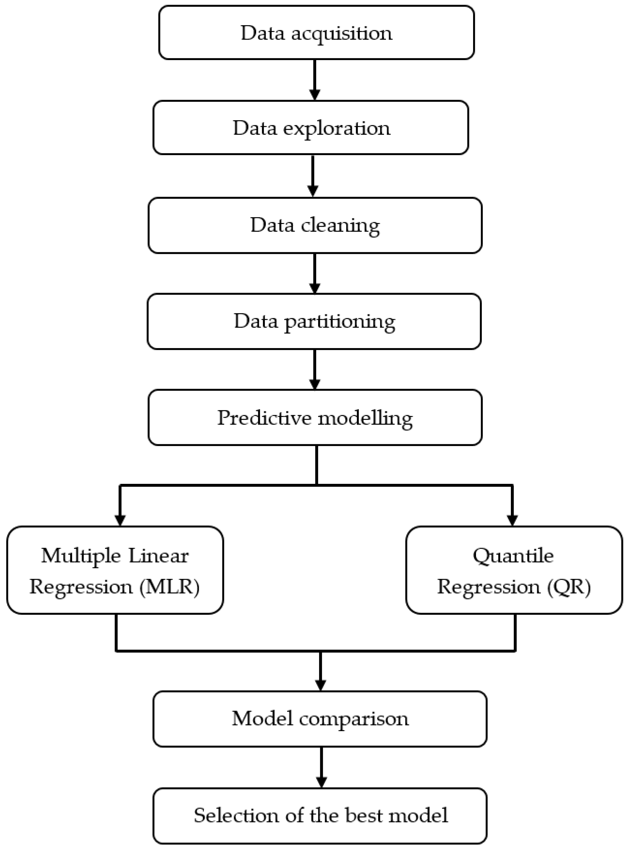
2. Materials and Methods

2.1. Study Areas

Three air quality monitoring stations situated in the west coast of the Malaysian peninsula were used in this study, namely Petaling Jaya, Melaka, and Pasir Gudang. These locations were chosen because they are directly affected by transboundary flow due to the location that they are situated in—the southern region of the Malaysian peninsula’s west bank, close to Indonesia. Table 1 details descriptions of the selected monitoring areas.

2.2. Air Pollutant Dataset

The air quality measurement records were received from the Air Quality Division of the Department of Environment (DoE), Malaysia. Continuous hourly data of air pollutants and meteorological parameters in the year that Malaysia experienced historic HPEs (1997, 2005, 2013, and 2015) were chosen for this study. Table 2 shows the air pollutants and weather parameters that were used in this study. An example of recorded data for each air quality parameter in 1997 is provided in Table S1: Air quality dataset for 1997.

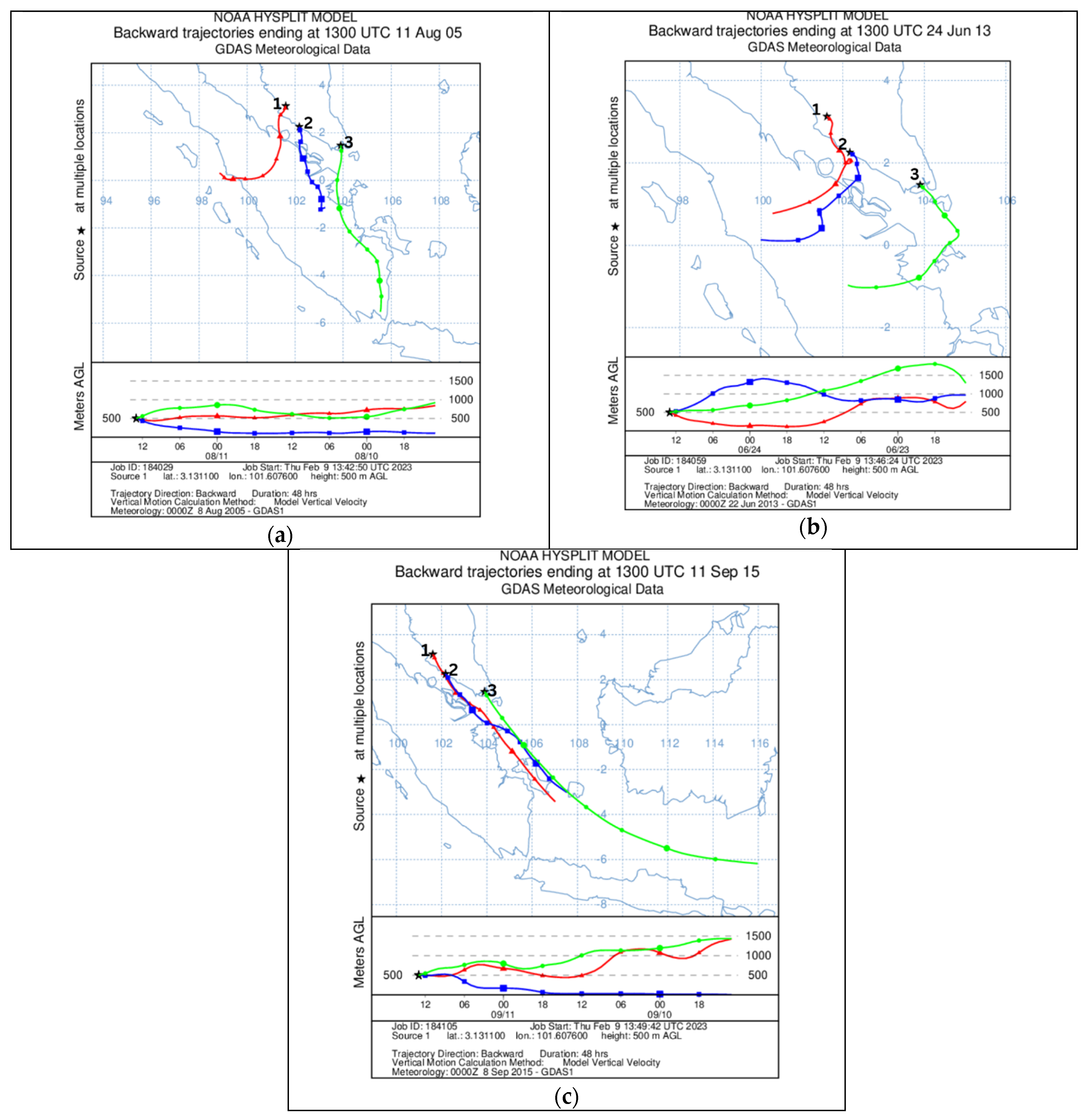
2.3. Trajectory Analysis

A trajectory analysis using hybrid single-particle Lagrangian-integrated trajectory (HYSPLIT) was conducted to determine the origin of the air masses’ backward trajectories for 48 h (2 days) during the haze events. The model used in this study is the NOAA (HYSPLIT-4). The model calculation method is a hybrid between the Lagrangian approach, using a moving frame of reference for the advection and diffusion calculations as the trajectories or air parcels move from their initial location, and the Eulerian methodology, which uses a fixed three-dimensional grid as a frame of reference to compute pollutant air concentrations [28].

2.4. Measure of Association using Pearson Correlation

Pearson correlation is an effective technique for calculating the relationship between two variables of interest. In this study, the relationship between PM10 with other pollutants and weather parameters was calculated using the Pearson correlation. The two variables x and y are measured using Pearson correlation analysis, which provides a correlation coefficient (r) between +1 and −1, with 1 denoting a positive correlation, 0 denoting no connection, and −1 denoting a negative correlation. The Pearson correlation equation is provided as:
r = ( x i x ¯ ) ( y i y ¯ ) ( x i x ¯ ) 2 ·   ( y i y ¯ ) 2
where
  • r = correlation coefficient
  • xi = values of the x-variable in a sample
  • x ¯ = mean of values of the x-variable
  • yi = values of the y-variable in a sample
  • y ¯ = mean of values of the y-variable
From the calculated r value, the degree of correlation can be identified. Table 3 shows the description of correlation using the following guide for the absolute value of “r” [29]:

2.5. Prediction Models

In this study, the next-day (PM10+24), the next-two-day (PM10+48) and the next-three-day (PM10+72) PM10 level during haze event were predicted. Figure 1 shows the modeling framework of this study. Data preparation include data acquisition, exploration, cleaning, and partitioning. The data acquisition pronounces the information of data and parameters included in this study (as presented in Section 2.2). Secondly, descriptive analysis, including central tendency (mean and median) and dispersion (standard deviation) analysis, was measured in data exploration. Then, data cleaning describes the technique involved in imputing the missing observation of the air quality monitoring dataset. In this study, expectation maximization (EM) was used to fill in the missing data, as this method was reported as the most consistent technique in estimating missing air pollutant observation [30]. Before developing the model, the original dataset was partitioned into two datasets for training and validation. Out of the total data, 80% was used to develop the model, where the rest of the data were used to validate the model. Parameters that had moderate to strong correlation (r ≥ 0.3) with PM10 level from the Pearson correlation analysis were used as the inputs for the prediction models. The details of the predictive models are discussed in Section 2.5.1 and 2.5.2 and the performance evaluation for comparing the performances of the model is described in Section 2.5.3.

2.5.1. Multiple Linear Regression (MLR)

MLR tries to simulate the connection between two or more independent variables and a dependent variable by fitting a linear equation to the observed data. MLR is one of the most used forecasting techniques. Equation (2) depicts a response (Y) based on a multiple regression model’s independent variables x1, x2…, xk.
Yi = β0+ β1X1 + …+ βk Xk + ϵi
where i is equal to n observations; Yi = the dependent variable (predicted PM10 level); Xk are the explanatory variables (air pollutants and weather parameters); β0 is the y-intercept (constant term); βk are the slope coefficients for each explanatory variable; ϵ = the model’s error term (also known as the residuals).

2.5.2. Quantile Regression (QR)

The target’s conditional median was calculated using quantile regression. When the prerequisites for linear regression—namely, linearity, homoscedasticity, independence, or normality—were not satisfied, the quantile regression method was applied. A certain value in the features variables may yield at any quantile (percent) using quantile regression, which is not only limited to computing the median. The quantile regression model equation is comparable in structure to the linear regression model. By minimizing the median absolute deviation, the optimum quantile regression line was discovered. In this research, quantile regression was applied and compared to the conventional MLR with specified percentile values of 0.25, 0.50, and 0.75. Taking a comparable structure to the linear regression model, the quantile regression model equation for the τth quantile is
Qτ(Yi) = β0(τ) +β1(τ)X1+ …+ βk(τ) Xk
where i is equal to n observations; τ = specified percentile value (0.25, 0.50, and 0.75); Yi = dependent variable (predicted PM10 level); Xk are the explanatory variables (air pollutants and weather parameters); β0 is the y-intercept with a dependency on the τ (constant term); βk are the slope coefficients for each explanatory variable with a dependency on the τ.

2.5.3. Performance Indicator

Performance measures were used to evaluate how well the regression models predicted the PM10 level at each research site. The performance measures used in this study are mean absolute error (MAE), root mean square error (RMSE), coefficient of determination (R2), and index of agreement (IA). A detailed description of performance indicators is tabulated in Table 4 [31].
  • where
  • n = total number of hourly measurements of particular site;
  • P i = predicted values of one set of hourly monitoring record;
  • O i = observed values of one set of hourly monitoring record;
  • P ¯ = mean of the predicted values of one set of hourly monitoring record;
  • O ¯ = mean of the observed values of one set of hourly monitoring record;
  • S p = standard deviation of the predicted values;
  • S O = standard deviation of the observed values of one set.

3. Results and Discussion

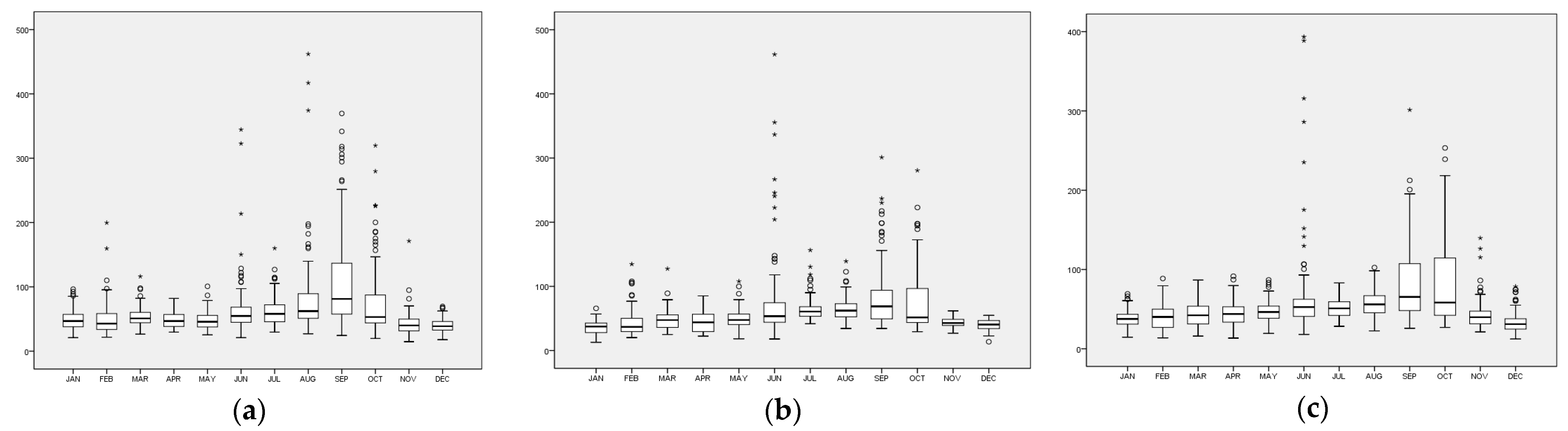
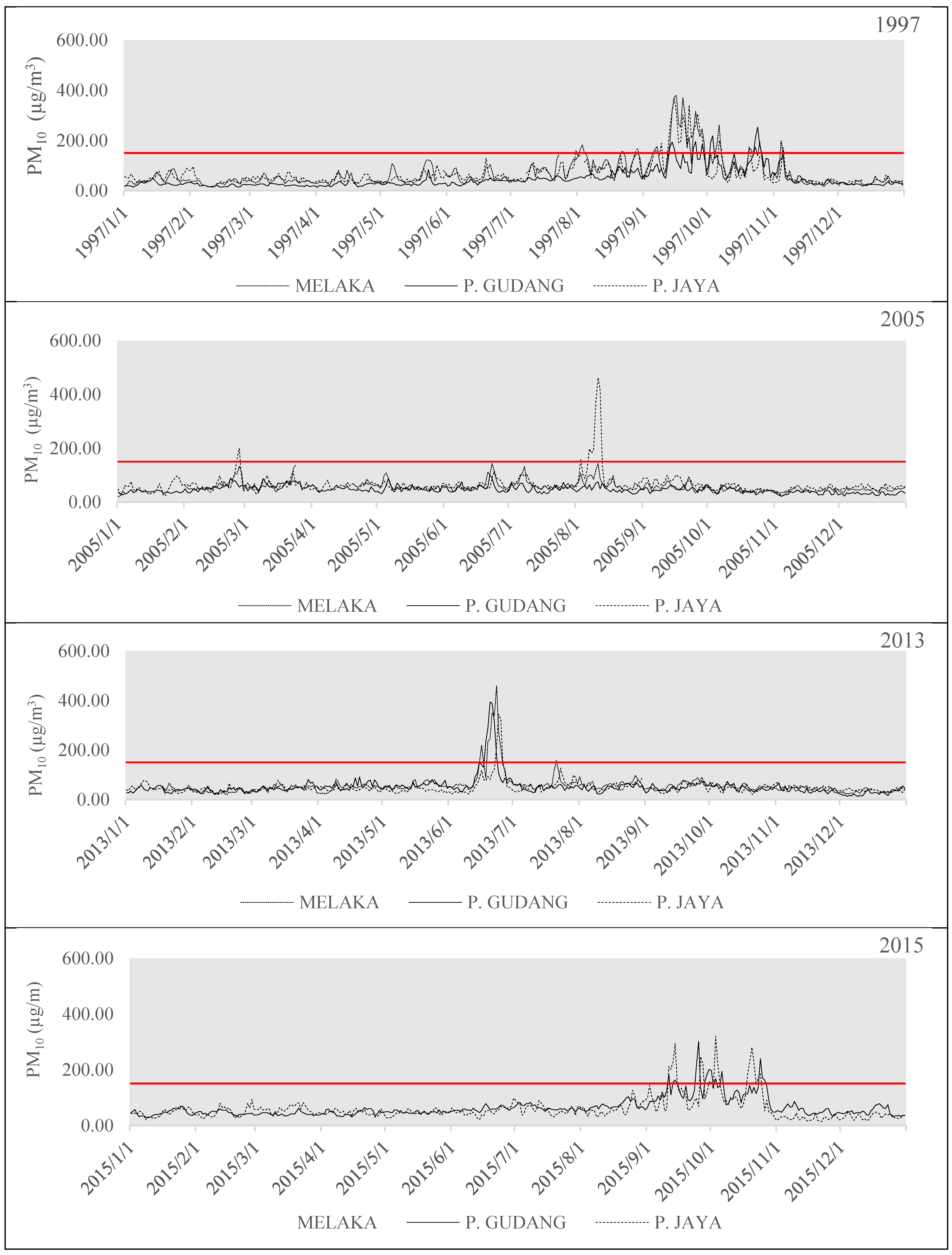
3.1. Variation of PM10 Level during Haze Event

Table 5 describes the data summary for PM10 concentration at Pasir Gudang, Melaka and Petaling Jaya, respectively, in 1997, 2005, 2013, and 2015. According to the recommended Malaysian ambient air quality guidelines (RMAAQG), the guideline for the 1-year average time of PM10 was 50 μg/m3. The mean PM10 levels for Pasir Gudang, Melaka, and Petaling Jaya were above the threshold value, especially in Melaka, with the highest annual concentration being recorded in 2005 (83 µg/m3). The mean values for all years exceeded the median values, indicating the existence of more a extreme concentration of PM10 in those years. Melaka and Pasir Gudang recorded maximum concentrations of PM10 in during haze event of 2013 with the measurement of 577 µg/m3 and 462 µg/m3, whereas Petaling Jaya recorded its highest PM10 level in 2005. Higher variability of PM10 level were recorded in Melaka and Petaling Jaya and Pasir Gudang with a standard deviation range of 27.4 µg/m3 to 61.6 µg/m3 compared to Pasir Gudang with a range of 13.7 µg/m3 to 39.9 µg/m3.
Figure 2 shows the box plots for PM10 concentration in Pasir Gudang, Melaka, and Petaling Jaya. Generally, it indicates that the measurement data were skewed to the right, and it indicates a distribution with a tail extending towards more positive value for the years 1997, 2005, 2013, and 2015 at Pasir Gudang, Melaka, and Petaling Jaya. Hence, it signified the occurrence of extreme values and outliers for the data sets. These values were due to the high particulate events (HPEs) experienced by Malaysia in those years. The highest exceedances or extreme PM10 concentrations can be observed in 2013. The haze phenomenon that occurred between June 2013 and October 2013—which was supposed to have the same effects as the smog in 1997—was to blame for this. The historic 1997 and the 2013 haze outbreaks were the two years that recorded a hazardous air pollutant index (API) in selected areas in Malaysia, including Melaka and Petaling Jaya. Pasir Gudang was not affected by the haze event in 2005, while Melaka was less affected than Petaling Jaya. The effects of the haze in 2015 were nearly the same in all locations.
Figure 3 displays the monthly boxplot of PM10 concentration in Pasir Gudang, Melaka, and Petaling Jaya in 1997, 2005, 2013, and 2015. Overall, the exceedances of PM10 concentration can be observed from June to September, i.e., during the southwest monsoon and in October during the intermonsoon period. Higher variability in PM10 concentrations in Petaling Jaya was recorded in September; meanwhile, Melaka and Pasir Gudang showed the highly variable PM10 concentrations in October. The slow wind during southwest monsoon and biomass burning affects the concentration of air particulate matter in Southeast Asia, specifically Malaysia [9]. The transboundary pollution due to biomass burning was transported from Indonesia. Studies by Juneng et al. [32] found that the exceedances in PM10 concentration coincided when regional low-level winds were primarily southerlies and southwesterlies, as well as when the region experienced a dry season. The lack of precipitation and high temperature may have contributed to the high concentrations of PM10 during the southwest monsoon [33].
To closely monitor the trend of haze event during these years, Figure 4 shows the timeseries plot for daily PM10 concentration in 1997, 2005, 2013, and 2015 at Melaka, Pasir Gudang, and Petaling Jaya. The solid red line designates the recommended Malaysia ambient air quality guideline (RMAAQG) for a 24 h averaging time, which is 150 µg/m3. The highest concentrations were observed in year 1997 at Petaling Jaya on 15th September and continued until the middle of September. A smoke-haze layer has formed in Malaysia due to transboundary pollution from the vegetation fires in Kalimantan and Sumatra during that time [34,35]. In addition, the El Niño phenomenon that year prolonged the dry season and caused the extended effects of the haze event in 1997. Bimodal peaks of PM10 concentrations are observed at Petaling Jaya in 2005 on 17th and 25th February. It was observed that Melaka and Pasir Gudang were not affected by the haze event in 2005. According to Soleiman et al. [36], the haze episode in August 2005 was more severe compared to the 1997 haze occurrence in peninsular Malaysia. The haze episode largely affected the entire Klang Valley and its nearby areas, where the air pollution index (API) in Klang Valley exceeded 500; thus, a haze emergency was declared in the area.
In 2013, the PM10 concentration started to rise, starting on 11th August, and high concentrations were observed at Melaka, Pasir Gudang, and Petaling Jaya on 25 June 2013, 23 June 2013, 21 June 2013, and 24 June 2013, respectively. The air quality in most regions within peninsular Malaysia worsened as a result of the transboundary pollution transported from massive land burning in Sumatra, Indonesia during that time [7]. In 2015, the peak PM10 concentrations at all four study locations started to increase from early September until the end of October in 2015. PM10 concentrations exceeded the RMAAQG with a fluctuating trend between September and October of that year. The air quality in Malaysia deteriorated due to huge land and forest fires in Sumatra and Kalimantan, Indonesia. It occurred during the period of the southwest Monsoon, coupled with an El Niño effect that resulted in a strong and prolonged drought observed across Southeast Asia [37]. The El Niño and drought, as well as the wide spread of the seasonal fires in Indonesia were greatly inflated, which caused large amounts of terrestrially-stored carbon to be released into the atmosphere [10]. According to the Department of Environment [4], for the first time in Malaysia’s history since 1997, 34 locations in the country experienced an unhealthy air quality level on 15 September 2015.
Figure 5 shows the backward trajectories of air parcels during the haze events in 2005, 2013, and 2015 at the studied areas. The trajectories were calculated for 48 h periods at a height of 500 m above ground level (AGL). Figure 5a indicates that during haze event in August 2005, the air masses travelled from the North Sumatra region to Petaling Jaya; meanwhile, the air masses arriving at Melaka and Pasir Gudang originated from the South Sumatra region. As shown in Figure 4, the haze event in 2005 only affected Petaling Jaya, as a high particulate event originated from Medan, Indonesia, which is located in the north of Sumatra. It was reported by Show and Chang [38] that 676 fire activities were recorded in Sumatra on 19 June 2013, which counted as a prominent peak hotspot. During this season, the southwesterly wind blowing from Sumatra to Malaysia and brought along thick smoke, covering Singapore and part of Malaysia for weeks [11]. Figure 5c demonstrates the backward trajectory in the middle of September 2015, showing the air masses travelling from the Kalimantan region. Khan et al. [39] reported that the release of CO flux in Kalimantan was about 6–7 times higher in strength than in Sumatra during the fire events of 2015; thus, the fire events in the Kalimantan area were likely to have more influence over the concentration of air pollutants at the study areas.

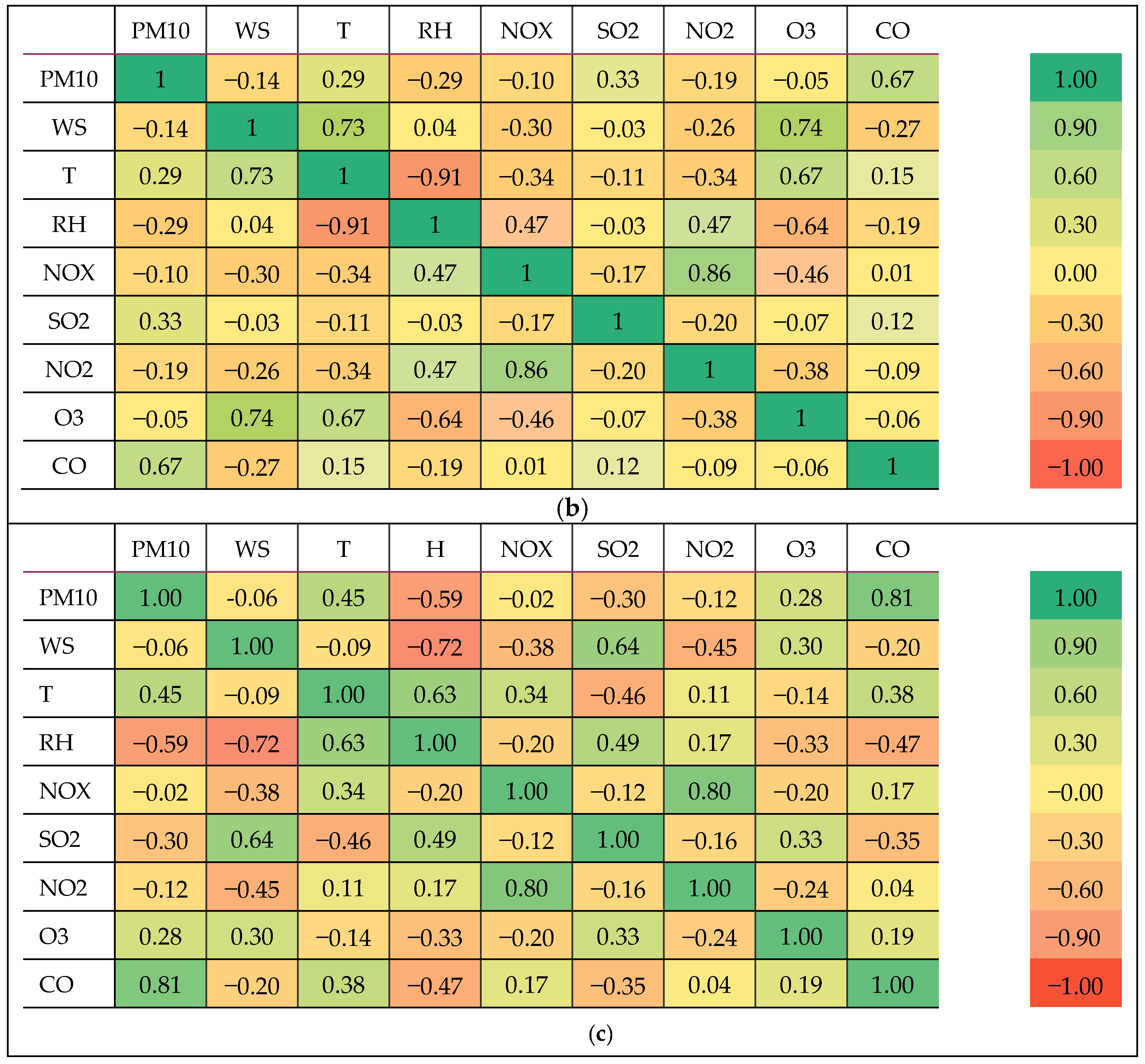
3.2. Association of PM10 Level with Other Air Pollutants and Weather Parameter during HPE

The heat map of the Pearson correlation in the three study areas is shown in Figure 6. The PM10 level in each location was found to have strong correlation with CO during haze events with the highest r value calculated in Petaling Jaya (r = 0.87). A strong association between PM10 level and CO may specify the influence from local anthropogenic sources such as emissions from traffic congestion and machinery usage due to the locations’ urban and industrial backgrounds. Moreover, the periodic land burning activities in the Sumatra region of Indonesia may have led to this situation as well. The huge land fires released huge amounts of terrestrially stored carbon into the atmosphere, primarily in the form of CO2, CO, and CH4 [10]. While this was happening, smoke travelled over large parts of Indonesia as well as other Southeast Asian countries including Malaysia [40]. The smoke came from peatland fires where over half had been cleared and drained for plantation development in particular (including oil palm and acacia for pulp and paper production). Drained, but still wet peat soils burn incompletely, at relatively low temperatures, which results in relatively high emissions of a mix of pollutants including particulate matter, carbon monoxide, and polycyclic aromatic compounds (PACs).
Weather parameters were observed to have strong and moderate relationships with PM10 levels in certain areas of study. A moderate positive correlation can be observed between PM10 level and temperature for all stations with the range from r 0.29 to 0.45. In addition, negatively strong (r = −0.6) and moderate correlation (r = −0.3) of PM10 level with relative humidity was detected in Pasir Gudang and Melaka, respectively. Other than CO, PM10 level was observed to have positive and negatively moderate correlation with SO2 in Melaka and Pasir Gudang, respectively. Grivas et al. [41] reported that the influence of diesel-powered vehicles to particle levels is suggested by the high correlation coefficients between PM10 and SO2. Sulfate is a main component of ambient particulate matter (PM) in the urban environment during haze episodes [41,42]. Among the pollutants, SO2 is an important precursor of sulfate and new atmospheric particle formation. Furthermore, high SO2 levels in ambient air also cause the formation of other sulfur oxides (Sox) that can react with other compounds in the atmosphere to form small particles, thus contributing to particulate matter pollution [43]. A relative humidity level of above 80% can significantly promote SO2 oxidation on CaCO3 particles and form CaSO4·2H2O crystals [43] where Malaysia has an average of RH of 75% and 95% [44].
For prediction model proposes, the parameters that were moderately to strongly correlated (r > 0.3) were used to develop the modified quantile regression model (Pearson–QR). Table 6 summarizes the parameters for each area.

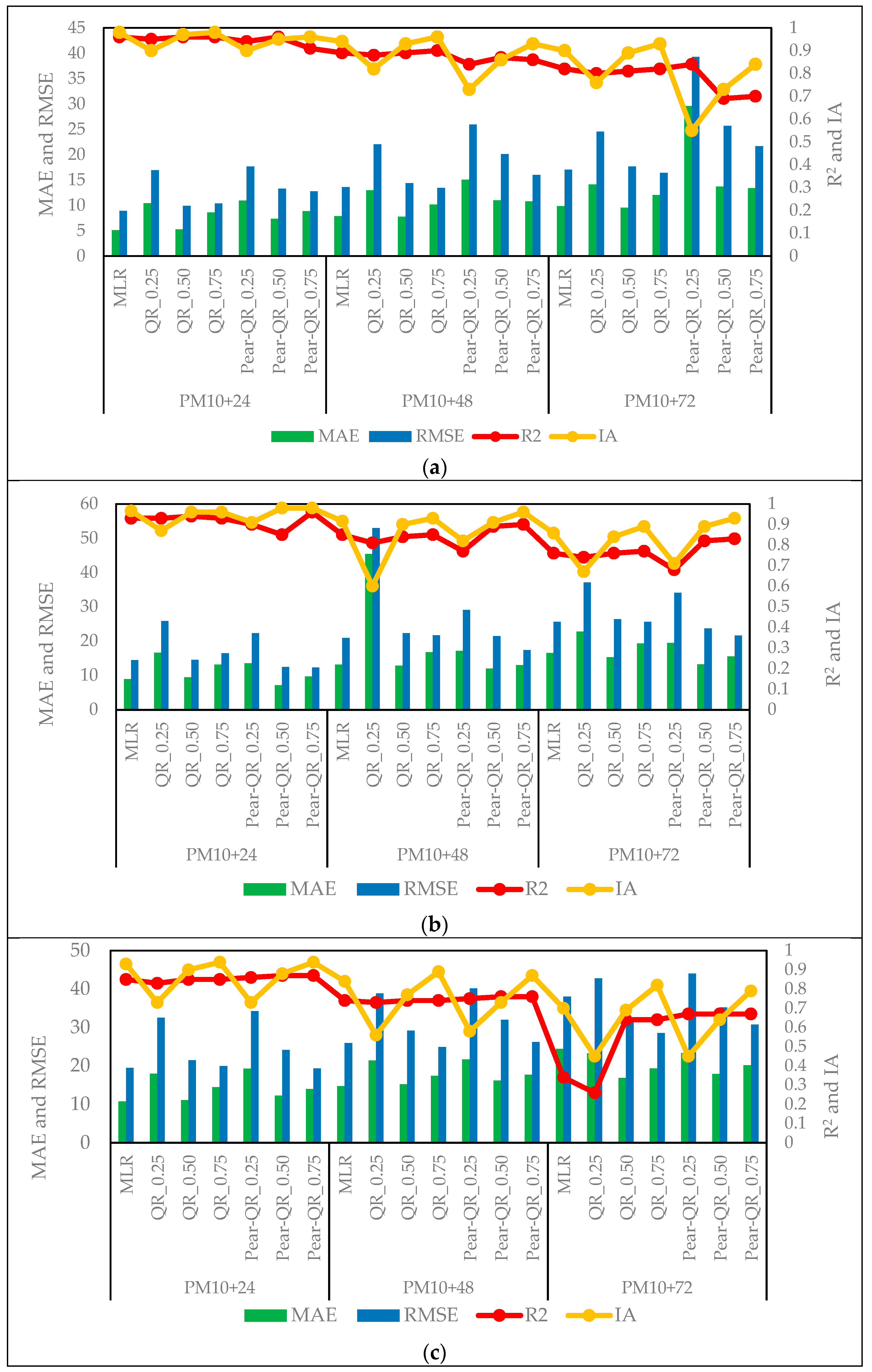
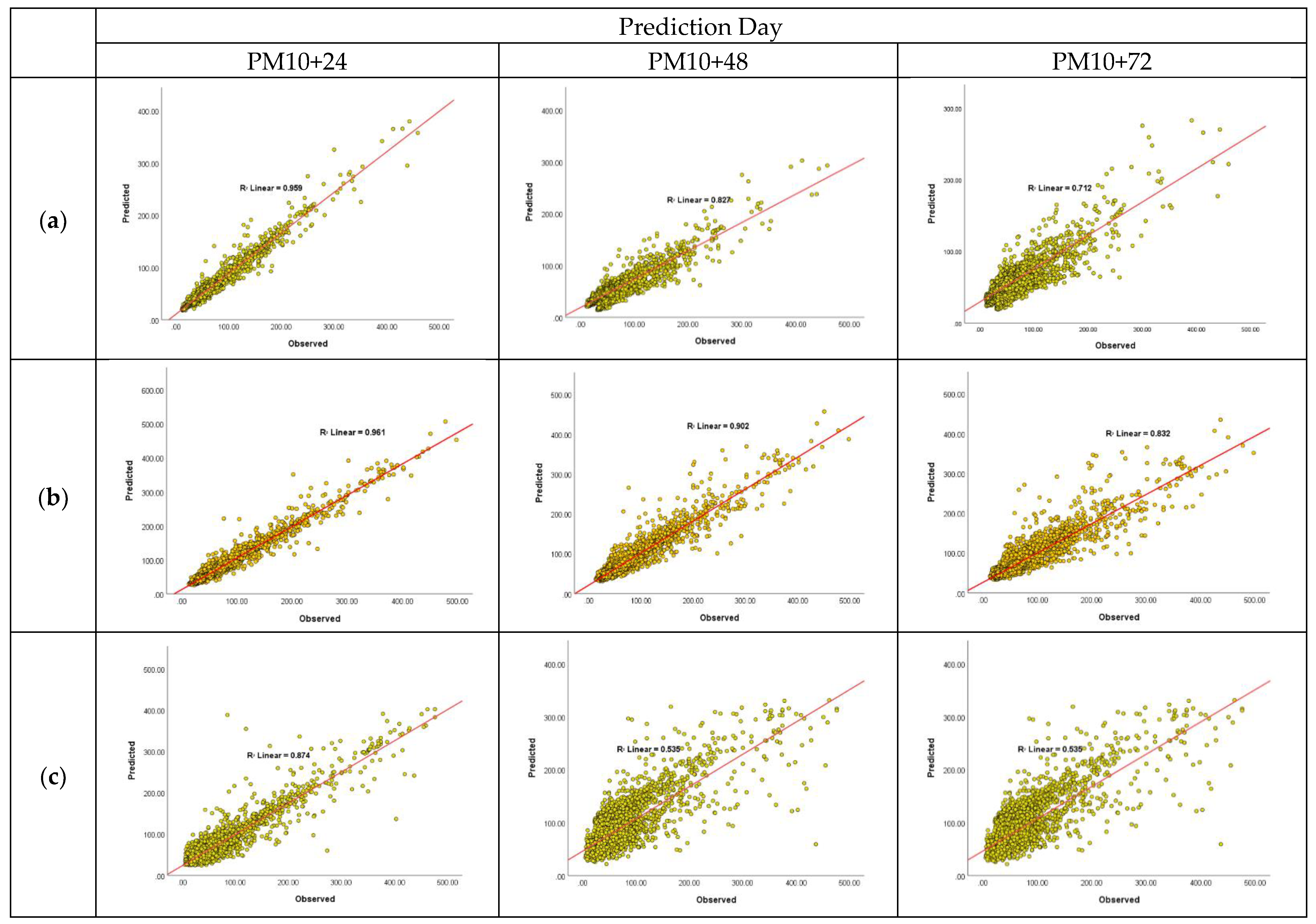
3.3. Predictive Models and Their Performances

Table 7 lists the predictive models (MLR, QR, and Pearson–QR) for the prediction of PM10 levels for the next day (PM10+24), the next two-days (PM10+48) and the next three-days (PM10+72) during a high particulate event. Obviously, in Melaka, for the MLR and QR predictive models, high constant values for parameters of NOx, SO2, NO2, and O3 were observed, ranging from 4.4 (constant for NOx) to 246 (constant for NO2). However, a smaller constant value for the CO parameter (ranging from 0.38 to 8.3) was calculated compared to the abovementioned parameters. In contrast, small values of constants for all selected parameters were detected in Pasir Gudang and Petaling Jaya if compared to Melaka. Conversely, higher values of constants, especially for the CO parameters of the Pearson–QR model, were noticed in Pasir Gudang and Melaka compared to other parameters where the values ranged from 0.68 to 3.9.
Table 8 presents the values of performance indicators once the predicted values were compared with the observed values. The bold values in the table indicate the best method with the best values of performance measures for each prediction time. Generally, when the prediction time increases from the next-day (PM10+24) to the next three-day (PM10+72), the error increases and the prediction of PM10 level is less accurate.
In Pasir Gudang, MLR was observed to be the most accurate model for the prediction of PM10+24 and PM10+48, whereas QR, with p = 0.75, was the best method for the prediction of PM10+72. It can be observed that for the QR model, p = 0.50 provides the best prediction for all prediction days. If compared to MLR, the modified Pearson–QR model at p = 0.50 showed the best performance for prediction of PM10+24 and PM10+48, while for PM10+72, the Pearson–QR at p = 0.75 provided a better prediction. This was due to the less extreme concentration of PM10 level in Pasir Gudang, as the mean average PM concentration was much lower than in other areas. Thus, MLR is suitable for implementation to model the overall mean concentration of PM10 with little emphasis on extreme conditions due to its assumption of normality [20].
Contrarily, in Melaka, the modified Pearson–QR model at percentile of 0.75 provided the most accurate prediction of PM10 levels for all prediction times. The performance of the QR regression at p = 0.50 was the best among all quantiles for the prediction of PM10+24 and PM10+48, whereas for PM10+72, QR at p = 0.75 provided better performance. In Petaling Jaya, QR models at the quantile of 0.75 provided the most accurate prediction for prediction of PM10+24 and PM10+48, whereas for PM10+72, the Pearson–QR at p = 0.75 provided the best prediction. MLR, on the other hand, provided a less accurate prediction compared to the QR and Pearson QR at p = 0.75. The QR has the ability to be more useful and precise, since the noncentral location of a distribution can be represented in all quantiles [23]. The QR has the capability to include models for all quantiles, evaluating the entire function and calculating the central tendency (such as mean, median, and mode) for the entire function of the variable of interest. The advantage of QR is its robustness and that it can also be adapted to unbalanced observational frequencies [45]. Table 9 summarizes the best method for each area according to prediction time.
In order to straightforwardly compare the performances of all the predictive models, Figure 7 summarizes the performance measures for all predictive models for the three-day prediction. The bar chart represents the error measure whereas the line describes the fitted line of observed and predicted PM10 concentration. Generally, all predictive models provided good prediction of PM10 concentration, especially for the next-day concentrations in Pasir Gudang and Melaka. However, Petaling Jaya showed slightly less accurate prediction of PM10 levels even on the first-day of prediction. For all areas, the QR method at p = 0.25 was observed to be the least accurate method for all three-day predictions. The QR at 0.25 describes the PM10 level at 25% of the total distribution of the dataset; hence, the prediction was too small if compared to the observed data. If compared to the mean value represented by MLR and QR at p = 0.75, they estimated the PM10 concentration according to the mean value and 75% from the total dataset, respectively. Thus, the predicted values of PM10 for these two methods were better than QR at 0.25. This finding is consistent with Ng and Awang [25], where better prediction of daily PM10 concentration in Petaling Jaya, Malaysia was calculated using a higher percentile compared to lower percentile of quantile regression, thus suggesting this method as one of the potential methods to be used for calculating air pollutants during haze events compared to usual atmospheric conditions. As for the modified QR model (Pearson–QR model), it is observed that less error was calculated for Pearson–QR at 0.75 if compared to the QR at 0.75 for prediction of PM10 concentration in Pasir Gudang and Melaka. Contrarily, in Petaling Jaya, the modified model (Pearson–QR at p = 0.75) recorded more error than the QR at p = 0.75 for predicted PM10 levels in the next two-day and the next three-day analyses.
Figure 8 describes the agreement between the predicted and observed PM10 level in the three areas using the best selected method as provided in Table 9. Generally, the prediction is more accurate for the short period, i.e., for the next-day (PM10+24) prediction compared to the next three-day (PM10+72) estimates. Out of the three areas, Petaling Jaya shows less agreement between the predicted and observed PM10 concentration that was calculated using Pearson–QR and QR, as the value of R (0.87) was significantly less if compared to the R-values in Pasir Gudang and Melaka (R = 0.96) for the first-day prediction. The Pearson–QR model at p = 0.75 predicted PM10 concentration very well in Melaka from the first day of prediction to the third day with the R-value > 0.80 whereas for Pasir Gudang, MLR model performed well in predicting PM10 level for the next day and the next two-day. Meanwhile, prediction for the next three-day of PM10 level in Pasir Gudang that was calculated using QR (p = 0.75) shows quite good estimates with an R-value of 0.7. Thus, it can be concluded that quantile regression is suitable for consideration as a reliable method of predicting PM10 concentration during unusual atmospheric conditions (haze) where the distribution of air pollutants were usually skewed to the right (due to extreme air pollutants concentration).

3.4. Comparing the Effectiveness of the Quantile Regression (QR) with Other Predictive Models

In this study, we aim to model the PM10 concentration during haze event using QR and a modified QR (Pearson–QR) and comparing the accuracy of the predictive models using MLR. From the previous section, it was proven that QR and Pearson–QR are reliable methods for use as predictive tools for estimating PM10 levels, especially during a high particulate event. QR and Pearson QR at p = 0.75 provided the most accurate prediction in Melaka and Petaling Jaya, in which QR at p = 0.25 provided the least effective prediction in all study areas.
In this section, the effectiveness of the QR models applied in this study are compared with recent studies that implemented QR, modified QR, MLR as well as machine learning algorithm. Table 10 shows selected recent studies on forecasting PM10 or PM2.5 concentration during haze and usual atmospheric conditions. Abdullah et al. [17] applied MLR to predict the next hour until the next three hours of PM10 concentration during transboundary haze in Malaysia. It was observed that the accuracy of the models were quite low, as the R2 value is <0.5 for the best selected model, i.e., the next-hour prediction. MLR is a linear model that is the most frequent predictive model used to forecast air quality. In addition to providing a simple mean linear relationship of PM10 concentration with other parameters, linear regression may not provide accurate predictions in some complex situations such as extreme value data [46]. A study by Ng and Awang [25] and Ul-Saufie et al. [47] used QR and a modified QR (coupling with a boosted regression tree), respectively, to forecast PM10 levels in peninsular Malaysia. Overall, the QR and BRT–QR provided more accurate prediction of PM10 in the specified study area. However, once comparing the R2 values for the BRT–QR model [47], the range of R2 values for this study was higher with the range from 0.98 to 0.93 for the next-day prediction. This might be due to less extreme PM10 concentration in the dataset since the study was conducted during usual atmospheric conditions. Hence, QR could not maximize its ability of describing the noncentral location of a distribution that can be represented in any quantiles, which allows QR to be more precise.
Machine learning is known as an effective technique for understanding the interdependence of climatic data and air pollution since it supports exploratory analysis of data without using an empirical model [48]. Worldwide, a lot of studies have been conducted to predict air pollutants using various kinds of machine learning algorithms. Recently, Tian et al. [49] proposed the deep belief–backpropagation neural network (DBN–BP) to predict next-day PM10 and PM2.5 levels during a smog-polluted weather period in Sichuan, China. Zhang et al. [50] claimed to develop an accurate prediction of the next-day PM2.5 level a during haze event using the gated recurrent unit (GRU) method with the accuracy increasing with the increase in its iteration. In Malaysia, lately Syaziayani et al. [51] proposed the support vector machine (SVM)–BRT to predict PM10 levels for three consecutive days. The accuracy of the proposed model was comparable with this study; however, this model was not developed for predicting PM10 during extreme an event. In summary, very limited-to-no study was known to predict PM10 levels during haze events using the QR method in Malaysia. Hence, this study has successfully developed QR models in Malaysia and the accuracy of the models were comparable with other predictive models including machine learning algorithms. Yet, this study can be enhanced by verifying the predictive models developed using the cross-validation method by the use of current air quality datasets. Since we do not have the suitable and recent air quality dataset (air quality with recent haze event) to verify the accuracy of the model, it is sufficient to compare the accuracy of the model using other related studies as presented in this subsection.

4. Conclusions

In this study, hourly air quality parameters in three locations (Petaling Jaya, Melaka, and Pasir Gudang), are situated in the west coast of peninsular Malaysia, during historical haze events in 1997, 2005, 2013, and 2015 were analyzed. The main purpose of this study was to investigate the performance of the quantile regression (QR) method in predicting the next-day (PM10+24), the next two-day (PM10+48) and the next three-day (PM10+72) PM10 levels at various percentiles including 0.25, 0.50, and 0.75. The Pearson correlation was calculated to identify the most influential parameters associated with PM10 concentration, specifically, in all study areas. It was found out that CO and temperature has a strong and moderate correlation with PM10 measurement records for all areas, respectively. Meanwhile, moderate association of SO2 was detected in Melaka and Pasir Gudang. From the Pearson analysis, parameters that had moderate to strong correlation with PM10 level (r > 0.3) were used as independent parameters to develop a PM10 predictive model, i.e., Pearson–QR. These models were compared with QR and multiple linear regression (MLR) to evaluate the applicability of the QR model in predicting unusual conditions in PM10 level, i.e., during a haze event. A number of performance measures such as mean absolute error (MAE), root mean squared error (RMSE), coefficient of determination (R2), and index of agreement (IA) were used to assess the performances of the models. It was proven that the Pearson–QR model at p = 0.75 outperformed the prediction of PM10 levels in Melaka for the next-day to next three-day periods with an R2 value >0.8. Meanwhile, QR with p = 0.75 was chosen as the best model in Petaling Jaya with the IA value ranging from 0.82 to 0.94. Contrarily, MLR outperformed the prediction of PM10 levels in Pasir Gudang due to less of extreme values in the dataset; hence, the overall mean concentration model was the best for representing PM10 concentration in this area. Thus, it was verified that the QR method can a reliable method for predicting air quality, especially during atmospheric unusual conditions, for example, during a high particulate event (HPE). Due to its ability to represent a noncentral location of a distribution that can be represented in any quantiles, QR can be seen as a preferred method for application, especially in nonnormal distributions of air pollutant concentration.
Despite the robustness of the QR method towards extreme data, one of the major drawbacks of quantile regression is that it is time-consuming to determine the best quantile for each model. Many training runs or experiments need to be conducted prior to obtain the best quantile for each dependent variable. Hence, application of a genetic algorithm could used to solve this problem. Genetic algorithms are a kind of optimization algorithm that can be used to solve problems in a variety of domains.

Supplementary Materials

The following supporting information can be downloaded at: https://www.mdpi.com/article/10.3390/atmos14020407/s1, Table S1: Air quality dataset for 1997.

Author Contributions

Conceptualization, N.M.N. and S.N.R.; methodology, N.M.N. and A.Z.U.-S.; software, N.A.A.A.R. and I.A.M.J.; validation, N.M.N., S.N.R. and A.Z.U.-S.; formal analysis, N.A.A.A.R. and I.A.M.J.; investigation, S.N.R.; resources, N.M.N.; data curation, S.N.R.; writing—original draft preparation, S.N.R. and S.E.B.; writing—review and editing, N.M.N. and A.V.S.; visualization, M.R.R.M.A.Z.; supervision, N.M.N.; project administration, A.V.S.; funding acquisition, A.V.S., P.V. and G.D. All authors have read and agreed to the published version of the manuscript.

Funding

This research was funded by Malaysian Ministry of Higher Education, grant number FRGS/1/2020/TK0/UNIMAP/02/53 (FRGS 9003-00837).

Institutional Review Board Statement

Not applicable.

Informed Consent Statement

Not applicable.

Data Availability Statement

Not applicable.

Acknowledgments

The author would like to thank the Department of Environment (DOE), Malaysia, for the air pollutant dataset.

Conflicts of Interest

The authors declare no conflict of interest.

References

  1. Latif, M.T.; Dominick, D.; Ahamad, F.; Khan, M.F.; Juneng, L.; Hamzah, F.M.; Nadzir, M.S.M. Long term assessment of air quality from a background station on the Malaysian Peninsular. Sci. Total Environ. 2014, 482, 336–348. [Google Scholar] [CrossRef] [PubMed]
  2. Abdullah, S.; Ismail, M.; Samat, N.N.A.; Ahmed, A.N. Modelling Particulate Matter (PM10) Concentration in Industrialized Area: A Comparative Study of Linear and Nonlinear Algorithms. ARPN J. Eng. Appl. Sci. 2019, 13, 8227–8235. [Google Scholar]
  3. Awang, M.B.; Jaafar, A.B.; Abdullah, A.M.; Ismail, M.B.; Hassan, M.N.; Abdullah, R.; Johan, S.; Noor, H. Air quality in Malaysia: Impacts, management issues and future challenges. Respirology 2000, 5, 183–196. [Google Scholar] [CrossRef] [PubMed]
  4. Department of Environment. Malaysia Environmental Quality Report 2015; Department of Environment, Ministry of Natural Resources and Environment: Putrajaya, Malaysia, 2016. [Google Scholar]
  5. Glover, D.; Jessup, T. Indonesia’s Fires and Haze: The Cost of Catastrophe; Institute of Southeast Asian Studies, International Development Research Centre: Ottawa, ON, Canada, 2000. [Google Scholar]
  6. Department of Environment. Malaysia Environmental Quality Report 2005; Department of Environment, Ministry of Natural Resources and Environment: Putrajaya, Malaysia, 2006. [Google Scholar]
  7. Department of Environment. Malaysia Environmental Quality Report 2013; Department of Environment, Ministry of Natural Resources and Environment: Putrajaya, Malaysia, 2014. [Google Scholar]
  8. Norela, S.; Saidah, M.S.; Mahmud, M. Chemical composition of the haze in Malaysia 2005. Atmos. Environ. 2013, 77, 1005–1010. [Google Scholar] [CrossRef]
  9. Sahani, M.; Zainon, N.A.; Wan Mahiyuddin, W.R.; Latif, M.T.; Hod, R.; Khan, M.F.; Tahir, N.M.; Chan, C.C. A case-crossover analysis of forest fire haze events and mortality in Malaysia. Atmos. Environ. 2014, 96, 257–265. [Google Scholar] [CrossRef]
  10. Huijnen, V.; Wooster, M.J.; Kaiser, J.W.; Gaveau, D.L.A.; Flemming, J.; Parrington, M. Fire carbon emissions over maritime southeast Asia in 2015 largest since 1997. Sci. Rep. 2016, 6, 26886. [Google Scholar] [CrossRef]
  11. Noor, N.M.; Yahaya, A.S.; Ramli, N.A.; Luca, F.A.; Al Bakri Abdullah, M.M.; Sandu, A.V. Variation of air pollutant (particulate matter-PM10) in peninsular Malaysia: Study in the southwest coast of peninsular Malaysia. Rev. Chim. 2015, 66, 1443–1447. [Google Scholar]
  12. Alifa, M.; Bolster, D.; Mead, M.I.; Latif, M.T.; Crippa, P. The influence of meteorology and emissions on the spatio-temporal variability of PM10 in Malaysia. Atmos Res. 2020, 246, 105107. [Google Scholar] [CrossRef]
  13. Payus, C.; Abdullah, N.; Sulaiman, N. Airborne Particulate Matter and Meteorological Interactions during the Haze Period in Malaysia. Int. J. Environ. Sci. Dev. 2013, 4, 398–402. [Google Scholar] [CrossRef] [Green Version]
  14. Afzali, A.; Rashid, M.; Sabariah, B.; Ramli, M. PM10 Pollution: Its prediction and meteorological influence in Pasir Gudang, Johor. IOP Conf. Ser. Earth Environ. Sci. 2014, 18, 012100. [Google Scholar] [CrossRef] [Green Version]
  15. Gvozdić, V.; Kovač-Andrić, E.; Brana, J. Influence of Meteorological Factors NO2, SO2, CO and PM10 on the Concentration of O3 in the Urban Atmosphere of Eastern Croatia. Environ. Model. Assess. 2009, 16, 491–501. [Google Scholar] [CrossRef]
  16. Akpinar, S.; Oztop, H.F.; Akpinar, E.K. Evaluation of relationship between meteorological parameters and air pollutant concentrations during winter season in Elaziğ, Turkey. Environ. Monit. Assess. 2008, 46, 21–24. [Google Scholar] [CrossRef] [PubMed]
  17. Abdullah, S.; Napi, N.N.L.M.; Ahmed, A.N.; Mansor, W.N.W.; Mansor, A.A.; Ismail, M.; Abdullah, A.M.; Ramly, Z.T.A. Development of multiple linear regression for particulate matter (PM10) forecasting during episodic transboundary haze event in Malaysia. Atmosphere 2020, 11, 289. [Google Scholar] [CrossRef] [Green Version]
  18. Fong, S.Y.; Abdullah, S.; Ismail, M. Forecasting of Particulate Matter (PM10) Concentration Based On Gaseous Pollutants And Meteorological Factors For Different Monsoons Of Urban Coastal Area In Terengganu. J. Sustain. Sci. Manag. 2018, 5, 3–17. [Google Scholar]
  19. Abdullah, S.; Ismail, M.; Fong, S.Y.; Ahmed, A.N. Evaluation for Long Term PM10 Concentration Forecasting using Multi Linear Regression (MLR) and Principal Component Regression (PCR) Models. EnvironmentAsia 2016, 9, 101–110. [Google Scholar]
  20. Ul-Saufie, A.Z.; Yahaya, A.S.; Ramli, A.; Hamid, H.A. Future PM 10 Concentration Prediction Using Quantile Regression Models. IPCBEE 2012, 37, 15–19. [Google Scholar]
  21. Baur, D.; Saisana, M.; Schulze, N. Modelling the Effects of Meteorological Variables on Ozone Concentration–A Quantile Regression Approach. Atmos. Environ. 2004, 38, 4689–4699. [Google Scholar] [CrossRef]
  22. Sayegh, A.S.; Munir, S.; Habeebullah, T.M. Comparing the performance of statistical models for predicting PM10 concentrations. Aerosol. Air Qual. Res. 2014, 14, 653–665. [Google Scholar] [CrossRef] [Green Version]
  23. Lingxin, H.; Naiman, D.Q. Quantile Regression; Sage Publications: London, UK, 2007. [Google Scholar]
  24. Kudryavtsev, A.A. Using quantile regression for rate-making. Insur. Math. Econ. 2009, 45, 296–304. [Google Scholar] [CrossRef]
  25. Ng, K.Y.; Awang, N. Quantile regression for analysing PM10 concentrations in Petaling Jaya. Mal. J. Fund. Appl. Sci. 2017, 13, 86–90. [Google Scholar] [CrossRef]
  26. Munir, S. Modelling the non-linear association of particulate matter (PM10) with meteorological parameters and other air pollutants—A case study in Makkah. Arab. J. Geosci. 2016, 9, 64. [Google Scholar] [CrossRef]
  27. Zhao, W.; Fan, S.; Guo, H.; Gao, B.; Sun, J.; Chen, L. Assessing the impact of local meteorological variables on surface ozone in Hong Kong during 2000–2015 using quantile and multiple line regression models. Atmos. Environ. 2016, 144, 182–193. [Google Scholar] [CrossRef]
  28. Stein, A.F.; Draxler, R.R.; Rolph, G.D.; Stunder, B.J.B.; Cohen, M.D.; Ngan, F. NOAA’s HYSPLIT Atmospheric Transport and Dispersion Modeling System. Bull. Am. Meteor. 2015, 96, 59–77. [Google Scholar] [CrossRef]
  29. Gogtay, N.J.; Thatte, U.M. Principles of correlation analysis. J. Assoc. Physicians India 2017, 65, 78–81. [Google Scholar]
  30. Sukatis, F.F.; Ul-Saufie, A.Z.; Noor, N.M.; Zakaria, N.A.; Suwardi, A. Estimation of Missing Values in Air Pollution Dataset by Using Various Imputation Methods. Int. J. Conserv. Sci. 2019, 10, 791–804. [Google Scholar]
  31. Ul-Saufie, A.Z.; Yahaya, A.S.; Ramli, N.A.; Hamid, H.A. Performance of multiple linear regression model for longterm PM10 concentration prediction based on gaseous and meteorological parameters. J. Appl. Sci. 2012, 12, 1488–1494. [Google Scholar] [CrossRef]
  32. Juneng, L.; Latif, M.T.; Tangang, F.T.; Mansor, H. Spatio-temporal characteristics of PM10 concentration across Malaysia. Atmos. Environ. 2009, 43, 4584–4594. [Google Scholar] [CrossRef]
  33. Juneng, L.; Latif, M.T.; Tangang, F. Factors influencing the variations of PM10 aerosol dust in Klang Valley, Malaysia during the summer. Atmos. Environ. 2011, 45, 4370–4378. [Google Scholar] [CrossRef]
  34. Heil, A.; Goldammer, J. Smoke-haze pollution: A review of the 1997 episode in Southeast Asia. Reg. Environ. Chang. 2001, 2, 24–37. [Google Scholar] [CrossRef]
  35. Fang, M.; Huang, W. Tracking the Indonesian forest fire using NOAA/AVHRR images. Int. J. Remote Sens. 1998, 19, 387–390. [Google Scholar] [CrossRef]
  36. Soleiman, A.; Othman, M.; Samah, A.A.; Sulaiman, N.M.; Radojevic, M. The occurrence of haze in Malaysia: A case study in an urban industrial area. In Air Quality; Rao, G.V., Raman, S., Singh, M.P., Eds.; Birkhäuser: Basel, Switzerland, 2003; pp. 221–238. [Google Scholar] [CrossRef]
  37. Samsuddin, N.A.C.; Khan, M.F.; Maulud, K.N.A.; Hamid, A.H.; Munna, F.T.; Rahim, M.A.A.; Latif, M.T.; Akhtaruzzaman, M. Local and transboundary factors’ impacts on trace gases and aerosol during haze episode in 2015 El Niño in Malaysia. Sci. Total Environ. 2018, 630, 1502–1514. [Google Scholar] [CrossRef] [PubMed]
  38. Show, D.L.; Chang, S.-C. Atmospheric impacts of Indonesian fire emissions: Assessing Remote Sensing Data and Air Quality During 2013 Malaysian Haze. Procedia Environ. Sci. 2016, 36, 6–9. [Google Scholar] [CrossRef] [Green Version]
  39. Khan, M.F.; Hamid, A.H.; Rahim, H.A.; Maulud, K.N.A.; Latif, M.T.; Nadzir, M.S.M. El Niño driven haze over the Southern Malaysian Peninsula and Borneo. Sci. Total Environ. 2020, 730, 139091. [Google Scholar] [CrossRef] [PubMed]
  40. Stockwell, C.E.; Jayarathne, T.; Cochrane, M.A.; Ryan, K.C.; Putra, E.I.; Saharjo, B.H.; Ati, D.N.; Israr, A.; Donald, R.B.; Isobel, J.S.; et al. Field measurements of trace gases and aerosols emitted by peatland fires in Central Kalimantan, Indonesia during the 2015 El Niño. Atmos. Chem. Phys. 2016, 16, 11711–11732. [Google Scholar] [CrossRef] [Green Version]
  41. Grivas, G.; Chaloulakou, A.; Samara, C.; Spyrellis, N. Spatial and Temporal Variation of PM10 Mass Concentrations within the Greater Area of Athens, Greece. Water Air Soil Pollut. 2004, 158, 357–371. [Google Scholar] [CrossRef]
  42. Liu, Y.; Tian, J.; Zheng, W.; Yin, L. Spatial and temporal distribution characteristics of haze and pollution particles in China based on spatial statistics. Urban Clim. 2022, 41, 101031. [Google Scholar] [CrossRef]
  43. Yue, Y.; Cheng, J.; Kang, S.; Stocker, R.; He, X.; Yao, M.; Wang, J. Effects of relative humidity on heterogeneous reaction of SO2 with CaCO3 particles and formation of CaSO4·2H2O crystal as secondary aerosol. Atmos. Environ. 2022, 268, 118776. [Google Scholar] [CrossRef]
  44. Saifullah, A.Z.A.; Yau, Y.H.; Chew, B.T. Thermal Comfort Temperature Range for Industry Workers in a Factory in Malaysia. Am. J. Eng. Res. 2016, 5, 152–156. [Google Scholar]
  45. Schlink, U.; Thiem, A.; Kohajda, T.; Richter, M.; Strebel, K. Quantile regression of indoor air concentrations of volatile organic compound (VOC). Sci. Total Environ. 2010, 408, 3840–3851. [Google Scholar] [CrossRef]
  46. Hashim, N.M.; Noor, N.M.; Ul-Saufie, A.Z.; Sandu, A.V.; Vizureanu, P.; Deák, G.; Kheimi, M. Forecasting Daytime Ground-Level Ozone Concentration in Urbanized Areas of Malaysia Using Predictive Models. Sustainability 2022, 14, 7936. [Google Scholar] [CrossRef]
  47. Shaziayani, W.N.; Ul-Saufie, A.Z.; Ahmat, H.; Al-Jumeily, D. Coupling of quantile regression into boosted regression trees (BRT) technique in forecasting emission model of PM10 concentration. Air Qual. Atmos. Health 2021, 14, 1647–1663. [Google Scholar] [CrossRef]
  48. Tong, W. Chapter 5-Machine learning for spatiotemporal big data in air pollution. In Spatiotemporal Analysis of Air Pollution and Its Application in Public Health; Li, L., Zhou, X., Tong, W., Eds.; Elsevier: Amsterdam, The Netherlands, 2020. [Google Scholar]
  49. Tian, J.; Liu, Y.; Zheng, W.; Yin, L. Smog prediction based on the deep belief-BP neural network model (DBN-BP). Urban Clim. 2022, 41, 101078. [Google Scholar] [CrossRef]
  50. Zhang, Z.; Tian, J.; Huang, W.; Yin, L.; Zheng, W.; Liu, S. A haze prediction method based on one-dimensional convolutional neural network. Atmosphere 2021, 12, 1327. [Google Scholar] [CrossRef]
  51. Shaziayani, W.N.; Ahmat, H.; Razak, T.R.; Zainan Abidin, A.W.; Warris, S.N.; Asmat, A.; Noor, N.M.; Ul-Saufie, A.Z. A Novel Hybrid Model Combining the Support Vector Machine (SVM) and Boosted Regression Trees (BRT) Technique in Predicting PM10 Concentration. Atmosphere 2022, 13, 2046. [Google Scholar] [CrossRef]
Figure 1. Modeling framework.
Atmosphere 14 00407 g001
Figure 2. The box plots for PM10 concentration in Pasir Gudang, Melaka, and Petaling Jaya.
Atmosphere 14 00407 g002
Figure 3. Monthly average boxplot of PM10 level in (a) Petaling Jaya, (b) Melaka, and (c) Pasir Gudang.
Atmosphere 14 00407 g003
Figure 4. Daily time series plot of PM10 level in Petaling Jaya, Melaka, and Pasir Gudang in 1997, 2005, 2013, and 2015.
Atmosphere 14 00407 g004
Figure 5. 48 h backward trajectories in Petaling Jaya, Melaka, and Pasir Gudang in (a) 2005, (b) 2013, and (c) 2015. Number 1 represents Petaling Jaya; 2 is Melaka; and 3 is Pasir Gudang.
Atmosphere 14 00407 g005
Figure 6. Heat map of the Pearson correlation matrix of PM10 levels with the other air pollutants and weather parameters for (a) Petaling Jaya, (b) Melaka, and (c) Pasir Gudang.
Atmosphere 14 00407 g006aAtmosphere 14 00407 g006b
Figure 7. Performance measures for prediction of the next-day (PM10+24), the next two days (PM10+48), and the next three days (PM10+72) in (a) Pasir Gudang, (b) Melaka, and (c) Petaling Jaya. MLR is multiple linear regression; QR_0.25 is quantile regression at p = 0.25; QR_0.50 is quantile regression at p = 0.50; QR_0.75 is quantile regression at p = 0.75; Pear-QR_0.25 is Pearson–quantile regression at p = 0.25; Pear-QR_0.50 is Pearson–quantile regression at p = 0.50; Pear-QR_0.75 is Pearson–quantile regression at p = 0.75.
Atmosphere 14 00407 g007
Figure 8. Relationship between observed and predicted value of PM10 concentration using the best predictive model (a) Pasir Gudang, (b) Melaka, (c) Petaling Jaya.
Atmosphere 14 00407 g008
Table 1. Details of study areas.
LocationStationCoordinatesBackground of Study Areas
Petaling JayaBandar Utama Primary School3.1311° N
101.6076° E
Heavy traffic particulars during the morning hour
Industrial area and
housing
MelakaBukit Rambai Secondary School2.2587° N
102.1729° E
Agriculture
Residential area and
housing
Pasir GudangPasir Gudang 2 Secondary School 1.4703° N
103.8956° E
Heavy industrial areas
Commercial land
Transportation and logistics
Table 2. Air quality parameters.
Air Quality and Weather
Parameters
SymbolUnit
Particulate matterPM10µg/m3
Ground-level ozoneO3ppm
Nitrogen oxidesNOxppm
Nitrogen dioxidesNO2ppm
Sulfur dioxidesSO2ppm
Carbon monoxideCOppm
TemperatureT°C
Relative humidityRH%
Wind SpeedWSkm/h
Table 3. Description of correlation related to the value of r.
Value of rDescription
0.0–0.3Weak
0.3–0.6Moderate
0.6–1.0Strong
Table 4. Performance indicator.
Performance IndicatorsEquationDescription
Mean absolute error (MAE) M A E = i = 1 n | P i O i | n When the value of MAE is closer to zero, it indicates better method.
Root mean square deviation (RMSE) R M S E = 1 n 1 i = 1 n ( P i O i ) 2 When the value of RMSE is closer to zero, it indicates better method.
Coefficient of determination (R2) R 2 = ( i = 1 n ( P i P ¯ ) ( O i O ) ¯ n . S p . S O ) When the value of R2 is closer to one, it indicates better method.
Index of agreement (IA) I A = [ i = 1 n ( P i O i ) 2 i = 1 n | P i O ¯ | + | O i O ¯ | 2 ] When the value of IA is closer to one, it indicates better method.
Table 5. Data summary for PM10 dataset in Pasir Gudang, Melaka, and Petaling Jaya in 1997, 2005, 2013, and 2015.
Place/
Year
Pasir GudangMelakaPetaling Jaya
199720052013201519972005201320151997200520132015
Total value, NValid863187158745871083378669866987598222872786598591
Missing1294515504239191153833101169
Mean47.746.595164.871.783.379.269.769.464.348.460.5
Median33.044.045.054.046.078.072.058.049.056.043.049.0
Standard deviation39.913.738.436.161.627.442.841.555.140.729.350.1
Minimum1119102713.02932242020175
Maximum268116462351415.0268577338393494372472
Table 6. Selected parameters for modified QR (Pearson–QR) model.
AreaSelected Parameter
Petaling JayaCO
Temperature
MelakaCO
RH
SO2
Temperature
Pasir GudangCO
RH
Temperature
SO2
Table 7. MLR, QR, and modified QR (Pearson–QR) equations for PM10 level prediction. The cream color represents the next-day prediction (PM10+24); blue represents the next two-day prediction (PM10+48); green represents the next three-day prediction (PM10+72).
AreaMethodQuantilePrediction DayPM10WSTRHNOxSO2NO2O3CO
Pasir GudangMLRMeanPM10+240.791−0.0970.228−0.0360.0150.0410.1070.0061.701
PM10+480.610−0.1810.788−0.006−0.0690.213−0.139−0.0710.800
PM10+720.482−0.3521.4280.095−0.1040.213−0.037−0.100−3.572
QR0.25PM10+240.471−0.115−0.111−0.1180.0210.2060.072−0.078−0.409
PM10+480.2720.0570.282−0.0330.1700.540.002−0.089−1.271
PM10+720.1690.0090.5740.0300.0250.428−0.100−0.139−0.810
0.50PM10+240.679−0.1120.154−0.035−0.0580.212−0.034−0.067−0.537
PM10+480.529−0.1930.424−0.029−0.1000.3550.084−0.045−2.021
PM10+720.429−0.1630.6730.025−0.0830.391−0.025−0.027−3.761
0.75PM10+240.772−0.1730.7320.082−0.0150.270−0.0180.0670.683
PM10+480.704−0.2430.6870.037−0.2030.2160.0930.036−1.092
PM10+720.580−0.1830.8600.089−0.1390.2840.0310.094−3.843
Pearson–QR0.25PM10+240.585 −0.108−0.086 0.125 −0.682
PM10+480.385 0.263−0.065 0.499 −1.373
PM10+720.310 0.5860.021 0.320 −1.958
0.50PM10+240.678 0.177−0.010 0.229 −0.487
PM10+480.533 0.4150.012 0.370 −1.981
PM10+720.429 0.6820.061 0.404 −3.580
0.75PM10+240.771 0.7000.110 0.319 1.011
PM10+480.702 0.6390.076 0.260 −0.601
PM10+720.587 0.8550.129 0.314 −3.896
MelakaMLRMeanPM10+240.771–0.275–0.004–0.195100.59629.012–53.14917.0900.483
PM10+480.663–0.221–0.121–0.20763.996204.937–91.66818.4321.021
PM10+720.594–0.205–0.009–0.19863.783208.651144.20841.8800.737
QR0.25PM10+240.5490.037–0.695–0.19321.083−52.16151.80061.6200.531
PM10+480.4300.084–1.023–0.245–5.578–143.956159.49650.740–0.477
PM10+720.3250.170–0.897–0.218–23.562–60.339246.02957.959–0.376
0.50PM10+240.766–0.132–0.201–0.1084.391–7.639105.47323.2181.313
PM10+480.578–0.105–0.342–0.11823.58–48.032159.49650.740.477
PM10+720.581–0.250–0.391–0.11713.265–79.94132.92524.141–0.655
0.75PM10+240.8600.2180.2270.06848.006173.93742.77722.2648.331
PM10+480.778–0.1660.134–0.08833.34686.98415.279–17.9326.667
PM10+720.732–0.05–0.135–0.11314.284162.53145.815–18.586.259
Pearson–QR0.25PM10+240.567 –0.685–0.201 –29.625 0.823
PM10+480.447 –0.932–0.249 –112.707 –0.340
PM10+720.857 0.196–0.068 –172.322 9.725
0.50PM10+240.776 –0.135–0.099 36.943 1.824
PM10+480.583 –0.296–0.105 –14.280 1.820
PM10+720.774 0.004–0.087 108.901 7.559
0.75PM10+240.857 0.196–0.068 –172.322 9.725
PM10+480.774 0.004–0.087 108.901 7.559
PM10+720.731 –0.254–0.110 164.423 6.914
Petaling JayaMLRMeanPM10+240.599–0.675–1.106–0.434–0.065–0.1630.5520.1473.867
PM10+480.457–0.68–1.506–0.5360.1190.3670.3600.082–0.11
PM10+720.353–0.281–1.846–0.5630.1290.8110.7250.01–1.647
QR0.25PM10+240.365–0.790–0.705–0.2730.0600.6590.624–0.1961.516
PM10+480.240–0.654–0.796–0.292–0.0481.0710.433–0.200–0.520
PM10+720.141–0.467–0.925–0.2790.0041.2500.563–0.076–1.194
0.50PM10+240.526–0.749–0.746–0.299–0.0900.1730.724–0.0091.477
PM10+480.358–0.436–1.277–0.415–0.0310.4750.276–0.0680.178
PM10+720.288–0.355–1.356–0.397–0.0010.7370.3130.084–1.410
0.75PM10+240.802–0.524–1.254–0.419–0.117–0.5900.4600.233–0.033
PM10+480.631–0.181–2.025–0.6090.050–0.4841.1590.111–0.903
PM10+720.497–0.085–2.053–0.6210.01–0.0110.2930.041–1.515
Pearson–QR0.25PM10+240.381 0.143 2.856
PM10+480.261 0.172 1.331
PM10+720.173 0.151 0.698
0.50PM10+240.554 0.176 1.863
PM10+480.386 0.166 0.329
PM10+720.322 0.095 0.995
0.75PM10+240.810 0.193 0.596
PM10+480.643 0.321 2.342
PM10+720.514 0.202 2.444
Table 8. Performance indicator values for the predicted PM10 levels. The cream color represents the next-day prediction (PM10+24); blue represents the next two-day prediction (PM10+48); green represents the next three-day prediction (PM10+72).
AreaMethodTimeMAERMSER2IA
Pasir GudangMLRPM10+245.118.900.960.98
PM10+487.8313.610.890.94
PM10+729.8617.030.820.90
QR0.25PM10+2410.4316.900.950.90
0.505.259.890.960.97
0.758.5810.330.960.98
0.25PM10+4812.9822.010.880.82
0.507.7314.370.890.93
0.7510.1713.430.900.96
0.25PM10+7214.1224.520.800.76
0.509.5317.630.810.89
0.7512.0016.420.820.93
Pearson–QR0.25PM10+2410.9217.640.940.90
0.507.3413.290.960.95
0.758.8612.750.910.96
0.25PM10+4815.0625.050.840.73
0.5010.9620.120.870.86
0.7510.7816.000.860.93
0.25PM10+7229.5639.250.840.55
0.5013.7125.650.690.73
0.7513.3721.640.700.84
MelakaMLRPM10+248.9314.430.930.9656
PM10+4813.0520.850.850.9162
PM10+7216.4825.550.760.8576
QR0.25PM10+2416.5625.770.930.87
0.509.5014.470.940.96
0.7513.0516.380.930.96
0.25PM10+4845.3952.930.810.60
0.5012.7722.270.840.90
0.7516.6721.650.850.93
0.25PM10+7222.7137.020.740.67
0.5015.2426.360.760.84
0.7519.2525.560.770.89
Pearson–QR0.25PM10+2413.4822.280.900.91
0.507.1212.430.850.98
0.759.7312.260.960.98
0.25PM10+4817.1329.030.770.82
0.5011.9221.430.890.91
0.7512.9017.340.900.96
0.25PM10+7219.3934.080.680.71
0.5013.1423.620.820.89
0.7515.4521.530.830.93
Petaling JayaMLRPM10+2410.7219.450.850.93
PM10+4814.6825.880.740.84
PM10+7224.4138.000.340.70
QR0.25 PM10+2417.9432.480.830.73
0.5011.0821.470.850.90
0.7514.4419.930.850.94
0.25PM10+4821.3538.830.730.56
0.5015.2029.120.740.77
0.7517.4224.870.740.89
0.25PM10+7223.2342.740.260.45
0.5016.8232.340.640.69
0.7519.2928.510.640.82
Pearson–QR0.25PM10+2419.2734.200.860.73
0.5012.5524.110.870.88
0.7513.9219.300.870.94
0.25PM10+4821.6640.120.750.58
0.5016.2031.960.760.73
0.7517.6926.170.760.87
0.25PM10+7223.2944.000.670.45
0.5017.8635.220.670.64
0.7520.1330.700.670.79
Table 9. Summary of the best prediction method.
AreaPrediction DayBest Method
Petaling JayaPM10+24Pearson–QR (p = 0.75)
PM10+48QR (p = 0.75)
PM10+72QR (p = 0.75)
MelakaPM10+24Pearson–QR (p = 0.75)
PM10+48Pearson–QR (p = 0.75)
PM10+72Pearson–QR (p = 0.75)
Pasir GudangPM10+24MLR
PM10+48MLR
PM10+72QR (p = 0.75)
Table 10. Recent studies forecasting PM concentration during haze and typical atmospheric conditions.
AreaMethodDependent
Variable
Prediction TimeDescription
Urban area in Malaysia [17]
  • MLR
PM10
  • Next h
  • Next two-h
  • Next three-h
  • Prediction was made for transboundary haze event using hourly dataset 2005 to 2015.
  • The best prediction time was the next-hour with the RMSE value of 127 and R2 value of 0.447.
Petaling Jaya [25]
  • QR (0.05 < p < 0.95 with the increment of p = 0.05)
  • MLR
PM10
  • Next day
  • The values of R τ 1 range from 0.29 at 0.05 quantile to 0.46 at 0.95 quantile.
  • This suggests that the PM10 distributions at high levels are better explained by the model com-pared to the lower quantiles.
  • This might suggest that the lagged air pollutants and meteorology played larger role in PM10 variation during haze period than any other time.
Peninsular Malaysia [47]
  • BRT–QR
PM10
  • Next 24 h
  • Next 48 h
  • Next 72 h
  • The results indicate that the QR has fulfilled the assumptions and the good model for BRT for predicting maximum daily PM10 concentration.
  • The performance measures show good prediction for next-day prediction with values of RMSE (9.33–22.25) and R2 (0.60–0.73).
  • Most of the results used 0.5 as the best quantile, which represents the median data, but 0.55 and 0.6 had also been chosen as the best quantile because the model has more number of outliers compared to the other models.
  • Overall, QR is an alternative loss function for BRT to predict the 3 days ahead of PM10 concentration and suitable for data containing influence outlier.
Sichuan, China [48]
  • Deep belief–backpropagation neural network (DBN–BP)
PM10PM2.5
  • Next 24 h
  • Proposed DBN-BP to predict PM10 and PM2.5 level during smog polluted weather in 2016–2017.
  • The analysis shows that the larger the number of hidden layers in the belief network, the higher the prediction accuracy. The prediction accuracy of PM2.5 is significantly higher than PM10.
  • The prediction effect of the DBN-BP neural network proposed is better compared to the traditional BP Neural Network.
China [49]
  • One-dimensional convolutional neural networks
  • Gated recurrent unit method (GRU)
PM2.5
  • Next 24 h
  • The convolutional neural network rises quickly in a short time, but the subsequent changes are not significant.
  • The accuracy rate of the GRU increases with the increase in the number of iterations. It can be said that the GRU neural network is more suitable for tasks with sufficient data volume and no requirement for training time.
Malaysia [50]
  • Support vector machine (SVM)–BRT
PM10
  • Next day
  • Next two-day
  • Next three-day
  • The BRT model was trained by utilizing maximum daily data in the cities of Alor Setar, Klang, and Kuching from the years 2002 to 2017.
  • The SVM–BRT model can optimize the number of predictors and predict PM10 concentration; it was shown to be capable of predicting air pollution based on the models’ performance with RMSE (10.46–32.60) and R2 (0.33–0.70).
  • This was accomplished while saving training time by reducing the feature size provided in the data representation and preventing learning from noise (overfitting) to improve accuracy.
West coast of peninsular Malaysia [This study]
  • QR
  • Pearson–QR
  • MLR
PM10
  • Next 24 h
  • Next 48 h
  • Next 72 h
  • Hourly air quality datasets during historical haze event were used to predict PM10 concentration.
  • Proposed modified QR method (Pearson–QR) and compared the performances of the predictive model with QR and MLR.
  • The QR and the Pearson–QR at percentile 75% provides the best prediction in areas with extreme PM10 concentration. Thus, the QR method a simple predictive model that can be used as a predictive tool during a haze event.
Disclaimer/Publisher’s Note: The statements, opinions and data contained in all publications are solely those of the individual author(s) and contributor(s) and not of MDPI and/or the editor(s). MDPI and/or the editor(s) disclaim responsibility for any injury to people or property resulting from any ideas, methods, instructions or products referred to in the content.

