Article

Comparison of PBL Heights from Ceilometer Measurements and Greenhouse Gases Concentrations in São Paulo

by
Amanda Vieira dos Santos
1,*,
Elaine Cristina Araújo
1,
Izabel da Silva Andrade
1,
Thais Corrêa
1,
Márcia Talita Amorim Marques
2,
Carlos Eduardo Souto-Oliveira
2,
Noele Franchi Leonardo
2,
Fernanda de Mendonça Macedo
3,
Giovanni Souza
1,
Pérola Pereira de Queiroz Lopes
1,
Gregori de Arruda Moreira
4,
Maria de Fátima Andrade
2 and
Eduardo Landulfo
1
1
Centro de Lasers e Aplicações (CELAP), Instituto de Pesquisas Energéticas e Nucleares IPEN-CNEN, São Paulo 05508-000, Brazil
2
Department of Atmospheric Sciences, Institute of Astronomy, Geophysics and Atmospheric Sciences, University of São Paulo, São Paulo 05508-090, Brazil
3
Faculdade de Tecnologia do Estado de São Paulo (FATEC), Praia Grande 11700-100, Brazil
4
Federal Institute of São Paulo (IFSP), Campus Registro, São Paulo 11900-000, Brazil
*
Author to whom correspondence should be addressed.
Atmosphere 2023, 14(12), 1830; https://doi.org/10.3390/atmos14121830
Submission received: 5 September 2023 / Revised: 16 October 2023 / Accepted: 17 November 2023 / Published: 16 December 2023
(This article belongs to the Special Issue Remote Sensing Measurement of Greenhouse Gases Emission)

Abstract

:
This paper presents a study conducted in São Paulo, Brazil, where the planetary boundary layer height (PBLH) was determined using ceilometer data and the wavelet covariance transform method. The retrieved PBLH values were subsequently compared with the concentrations of CO2 and CH4 measured at three distinct experimental sites in the city. The period of study was July 2021. This study also included a comparison between ceilometer data and lidar data, which demonstrated the favorable applicability of the ceilometer data for PBLH estimation. An examination of the correlation between changes in average CO2 concentrations and PBLH values revealed stronger correlations for the IAG and UNICID stations, with correlation coefficients (ρ) of approximately −0.86 and −0.85, respectively, in contrast to the Pico do Jaraguá station, which exhibited a lower correlation coefficient of −0.42. When assessing changes in CH4 concentrations against variations in PBL height, the retrieved correlation coefficients were approximately −0.78 for IAG, −0.66 for UNICID, and −0.38 for Pico do Jaraguá. The results indicated that CO2/CH4 concentrations are negatively correlated with PBL heights, with CO2 concentrations showing more significant correlation than CH4. Additionally, among the three measurement stations, IAG measurements displayed the most substantial correlation. The results from this study contribute to the understanding of the relationship between PBLH and greenhouse gas concentrations, emphasizing the potential of remote sensing systems like ceilometers in monitoring and studying atmospheric processes.

1. Introduction

The atmospheric boundary layer or planetary boundary layer (PBL) is the lowermost region of the troposphere. Such a region is directly influenced by the Earth’s surface, so that it is fundamental in the exchange process of momentum, heat, and moisture between the atmosphere and the surface [1]. The vertical height of the PBL (PBLH) is influenced by weather conditions and topography, varying in time and space, presenting a daily and seasonal cycle strongly influenced by the atmospheric stability and surface heat fluxes [1]. The PBLH is a key parameter in pollutant dispersion studies, as well as weather forecasting, air quality, and climate modeling [2,3]. The PBL dynamics affect the greenhouse gases (GHG) concentration near the surface [4,5] because the top of this layer acts as a lid, partially blocking the transport and dispersion process to the free atmosphere (FA). Therefore, the PBL is often used as a fundamental parameter to estimate the vertical fluxes of pollutants and greenhouse gases.
However, it is not possible to measure the PBLH directly; in fact, it can be obtained by using as a proxy some vertical profiles of atmospheric variables, such as particle concentrations, relative humidity, wind speed, and potential temperature. Then, PBLH can be estimated by many different methodologies, using remote sensing instruments such as lidar (elastic and/or Doppler [6]), ceilometers, wind-profiling radars [7], microwave radiometers [8], and mainly radiosondes, the most widely applied method. PBLHs measured from radio soundings are often estimated using methods like the Richardson number [9], which is based on the wind and temperature profiles. Although these estimates are generally accurate, unfortunately radiosondes lack the necessary temporal (they are often launched twice per day) and spatial resolution for effectively detecting the PBLH daily cycle. On the other hand, lidar systems and ceilometers are powerful tools that can be applied in this kind of study [10,11,12,13,14,15]. These kinds of remote sensing systems allow for long-term measurements with high temporal and spatial resolutions [16,17,18,19,20,21]. However, due to the high complexity of the PBL dynamics, the PBLH detection depends on mathematical methods like the maximum gradient method [22,23,24], the variance method [24,25], the wavelet covariance transform method [7,12,16,20,26,27], and ideal profile fitting [28,29].
Although ceilometers are simpler than elastic lidars, they are reasonable tools for automatic PBLH evolution retrievals. The ceilometers utilize a single wavelength and typically employ a less intense laser source, thereby offering a smaller instrument range and producing a signal with more noise. However, they operate continuously and can be fully automated, making them good alternatives to more powerful lidar systems. Although their performance is limited when compared to lidar systems, the usual algorithms of estimation for the PBLH still can be used with ceilometers [30].
When investigating GHG concentrations in the PBL, a knowledge of the PBL height is a useful tool to learn about sinks and sources of GHGs. For instance, concentrations of carbon dioxide (CO2), a long-lived anthropogenic GHG, are influenced by the interactions happening near the surface, such as photosynthesis and evapotranspiration, and by the PBLH [5,31,32]. Carbon dioxide, in particular, accounts for most of the warming effect on the climate [33,34,35,36], and methane contributes to roughly 20% of the global warming attributed to all well-mixed GHGs [35,36,37]. A substantial portion of the longwave radiation emitted by the surface is absorbed by methane. Therefore, this GHG shows a considerable trend to affect the radiative forcing [38]. Comprehending the influence of atmospheric CH4 and CO2 on Earth’s climate, including tracking their sources, sinks, global dispersion, and long-term trends, remains crucial for future climate assessment.
Cities play a substantial role in the emission of GHGs, accounting for approximately 70% of CO2 anthropogenic emissions [39]. The Metropolitan Region of São Paulo (MRSP) has around 19 million inhabitants and a large number of vehicles, which are the main source of air pollutants emission in the region and currently number seven million. Comprehending the urban impact is essential for the creation of mitigation policies. Nonetheless, calculating the total amount of pollutants emitted is a complex challenge, since their emission is influenced not only by human activities but also affected by the interaction between land and surface. This study aims to investigate the influence of the PBL height on CO2 and CH4 concentrations measured in São Paulo during July 2021. PBLHs were obtained using a ceilometer and applying the wavelet covariance transform method, and CO2 and CH4 concentrations were obtained with CRDS instruments.

2. Materials and Methods

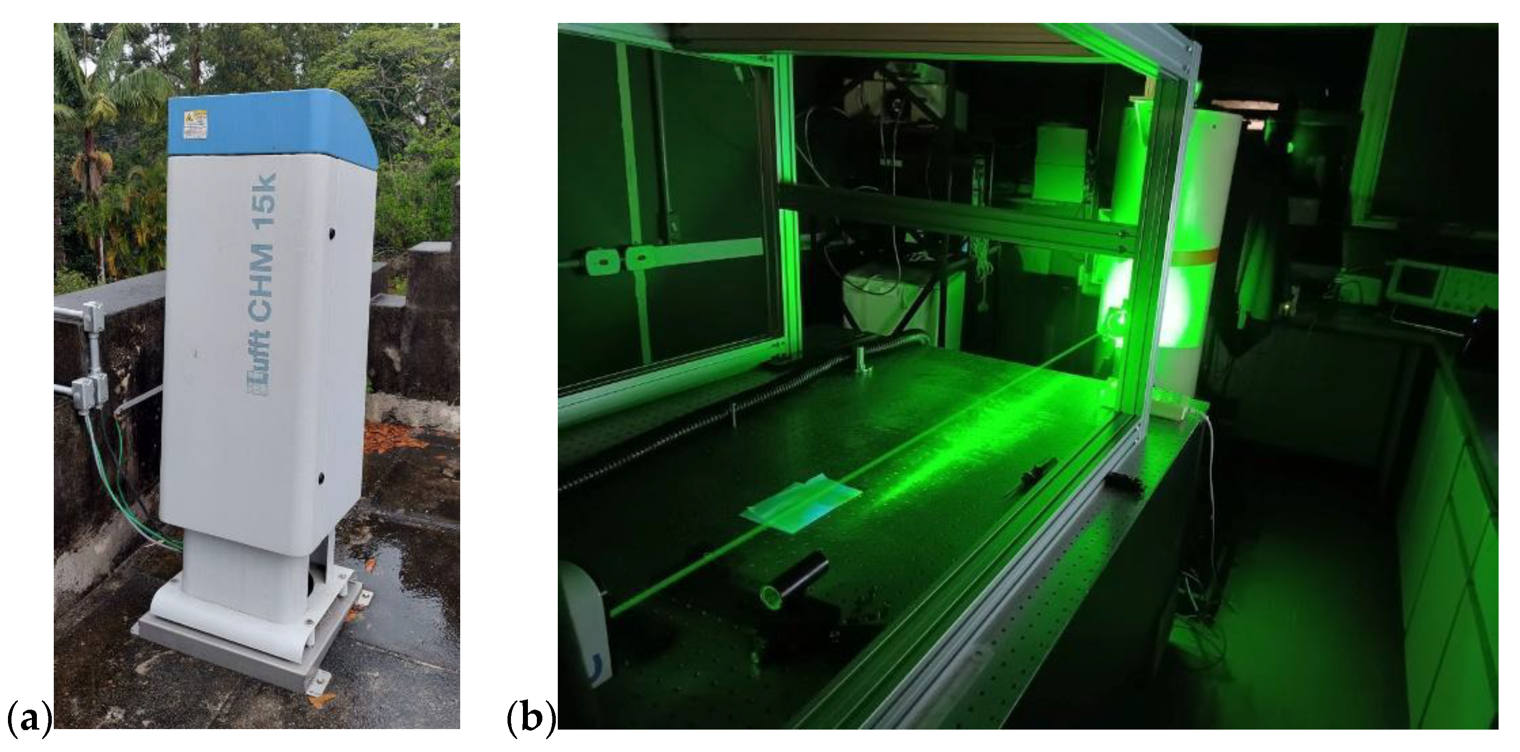
2.1. Data and Instrumentation

The ceilometer system used in this study was the CHM 15k Lufft ceilometer (Figure 1a), which operated uninterruptedly during the period selected for analysis. It utilizes an eye-safe system equipped with a solid-state Nd:YAG laser that emits radiation at a single infrared wavelength of 1064 nm, with a maximum range of 15 km. The ceilometer provides data with a vertical resolution of 15 m and a temporal resolution of 15 s. For more detailed information, please refer to the instrument manual, available at (https://www.lufft.com/download/manual-lufft-chm15k-en/, accessed on 10 October 2023).
The lidar system used was the Metropolitan São Paulo Lidar 1 (MSP1) system (Figure 1b). It uses a pulsed Nd:YAG, operating at a fundamental wavelength of 1064 nm, generating second and third harmonics at 532 nm and 355 nm, and with a repetition frequency of 10 Hz. The instrument was run with a temporal resolution of 1 min and a spatial resolution of 7.5 m. The MSP1 is located in a suburban setting at the Center for Lasers and Applications of the Energy and Nuclear Research Institute (IPEN) building (23°34′ S, 46°3′ W, 782 m above sea level).
The network monitoring greenhouse gases in the São Paulo megacity, part of the Metroclima Project, is the first GHG network in South America. This network utilizes wavelength-scanned cavity ring-down spectroscopy (CRDS) instruments located at multiple sites in the city. CO2, CH4, and water vapor concentration measurements are carried out at all sites, while CO concentrations are measured at one of them. Table 1 describes the three monitoring sites from which data were used in this study (http://www.metroclima.iag.usp.br/, accessed on 4 September 2023).
The concentrations of CO2 and CH4 were measured using the Picarro Cavity Ring-Down spectrometer, manufactured by Picarro Inc. (Santa Clara, CA, USA). This high-precision greenhouse gas (GHG) analyzer enables concurrent measurements of CH4 and CO2 at parts-per-billion (ppb) levels and water (H2O) at parts-per-million (ppm) levels, while demonstrating minimal drift. For further details about this instrument, please refer to the manufacturer’s website at https://www.picarro.com/g2401_gas_concentration_analyzer (accessed on 10 October 2023).

2.2. Locations

The Metropolitan Area of São Paulo (MASP), situated at 23°33′ S, 46°38′ W, with an elevation of 760 m above sea level, is the most densely populated metropolis in Brazil, the Americas, and the Southern Hemisphere [40]. The MASP major pollutants contribution is related to the anthropogenic emissions, due to the MASP’s enormous population and its industrial and vehicular activities. Therefore, it becomes crucial to monitor the presence of atmospheric pollutants and GHGs, study their transport and dispersion, and continuously track the development of the planetary boundary layer (PBL) in this polluted region. Such monitoring efforts yield valuable insights into local air quality. The primary sources of pollutants in the MASP stem from burning of fossil fuels, primarily due to the presence of vehicles exceeding 7 million in number [41]. Vehicular traffic serves as the main contributor to pollutant emissions within the city. Additionally, air pollution in São Paulo is further influenced by biomass burning in nearby regions. Geographically located in the southeastern part of Brazil, São Paulo experiences a humid subtropical climate (Cwa). The city’s summers (January–March) are warm and wet, while winters (July–September) are mild and dry [41].
Planetary boundary layer height data were obtained from ceilometer measurements located at the CIENTEC site (located at 23°39′ S, 46°37′ W). The CHM 15k ceilometer was positioned on the rooftop of the Museum of Meteorology within the Science and Technology Park (CIENTEC) of the University of São Paulo. Situated in a suburban environment, the site is approximately 810 m above sea level.
CO2 and CH4 quantification were measured at three sites in the MASP area using CRDS Picarro spectrometers. A suburban area called IAG, which has the coordinates of 23°33′ S, 46°44′ W and 731 m of elevation above sea level, was one of the places used to acquire these gasses. At this place, more precisely at the rooftop, the acquisition started. As mentioned, the coordination data were exactly at the University of São Paulo, near an urban highway located in close proximity to the site, around 1 km away, experiencing an average daily traffic volume exceeding 250,000 vehicles. UNICID was another place of acquisition, at 23°32′ S, 46°33′ W, with 741 m of elevation above sea level, which was carried out at an inlet at the top of the building. An extremely busy highway is located near this site, along with an elevated subway station. In addition, a domestic wastewater treatment site can be found about 2.5 km from this site. The site of Pico do Jaraguá (23°27′ S, 46°45′ W) was located in the air quality monitoring station of the Environmental Company of the State of São Paulo (CETESB) in Pico do Jaraguá (Jaraguá Peak). It is located in the highest places of the MASP and surrounded by the Atlantic Forest reserve called Jaraguá. This is located at 1079 m above sea level. The locations and distances between the measurement sites are shown in Figure 2:

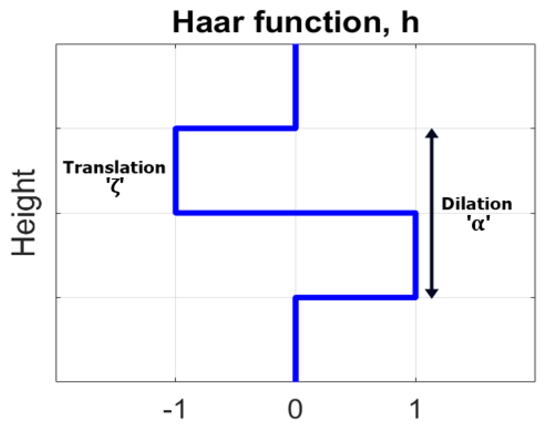
2.3. PBLH Retrieval Method

The algorithmic method of wavelet covariance transform (WCT) was used, with certain modifications to enhance retrieval in different conditions. The selection of this algorithm was based on its demonstrated effectiveness across diverse meteorological scenarios and its flexibility for adjustment. The WCT method is usually used to obtain PBL heights from lidar data by detecting abrupt variations in the range-corrected signal which correspond to variations in aerosol concentration [16]. For that, the covariance transform W f ( α , ζ ) measures the similarity between the Haar function and the RCS. It is defined by Equation (1):
W f α , ζ = 1 α z ζ z α R C S z h z ζ α d z ,
where h z ζ α corresponds to the Haar function, expressed as:
h z ζ α = { 1 : ζ α 2 z ζ   1 : ζ z ζ + α 2   0 : O t h e r   c a s e s ,
RCS is the range-corrected signal P z z ² obtained by an instrument such as a lidar or ceilometer, where P(z) is the measured signal as a function of height, and z is the distance from the instrument. The lower and upper limits of the signal are giving by z α and z ζ , respectively; α is the dilation of the function and ζ is the vertical translation of the function [26].
The maximum global value of W f α , ζ corresponds to the height where an abrupt change becomes apparent in the lidar or ceilometer signal. This indicates the location where the backscatter profile and the Haar wavelet function exhibit the highest similarity. Prior to applying the method, the initial conditions α and ζ must be defined. The dilation of the Haar function, α , defines the range within which the algorithm seeks abrupt changes in the RCS profile. Selecting an appropriate value for α can be crucial for accurately determining the PBLH, particularly in non-ideal conditions. Small values of α can result in the detection of aerosol layers due to the small gradients they generate. Low clouds and noise also generate local maxima, impairing the retrieval of the PBLH, especially for small values of α . In clear-sky conditions, the value of α is not as critical for an accurate retrieval of the PBLH, as it is unlikely that multiple maxima will be present in the signal. The center of the Haar function is given by the value of ζ . As the location where the function is centered is translated by ζ , the value of α should be greater than the value of ζ . A representation of the Haar function can be seen in Figure 3.
A few adjustments were implemented to enhance result accuracy. During the diurnal period and when confronted with a dense or several strata of cloud or aerosol formations, the CHM15k’s backscattering signal may encounter high noise due to signal attenuation. To improve the signal-to-noise ratio and facilitate change detection, a 30 min average was applied to the backscatter profiles. The CHM 15k ceilometer provides cloud base height estimates for each of its signal profiles. While these results are automatically generated and may occasionally contain errors, they serve a valuable purpose in screening the profiles used in the analysis to identify low clouds that could interfere with PBLH retrieval.
The WCT method can be applied in complex cases [12]. Although the method’s accuracy may be compromised in cases involving multiple aerosol layers [42], it presents several advantages, such as being less affected by noise, and ease of automation [16], as the ‘ α ’ and ‘ ζ ’ parameters can be fine-tuned for improved PBL height identification in various circumstances.

3. Results

Throughout July 2021, the CHM 15k ceilometer operated continuously at CIENTEC. PBL heights were estimated using the WCT method for all days without cloud cover. Concurrently, instruments deployed at three distinct sites in São Paulo retrieved measurements of CO2 and CH4 concentrations.

3.1. PBLH Estimation

To explore the possibility of using the same estimated PBLH for all stations, as opposed to individual estimations for each location, the results obtained from the CHM 15K ceilometer and the MSPI lidar on 26 July 2021 were compared. On this specific date, daytime cloud cover was minimal, and the incoming air masses at all site locations displayed similar origins, as indicated by HYSPLIT backward trajectories. Additionally, there were no significant reports of biomass burning events in the area during that period. Figure 4a,b show the range-corrected signal obtained from both instruments on 26 July, along with the corresponding PBLH values derived using the WCT method.
The PBL exhibits a customary manifestation during cloudless days, expanding from the middle of the morning to the early hours of the afternoon (local time, UTC-3), with the PBL top reaching its peak height during mid-afternoon. This behavior in PBLH is associated with the rise in temperature attributed to increasing solar radiation during morning and afternoon. At around 20:00 UTC, data from both instruments show the development of the residual layer, which can introduce challenges when identifying the PBLH. As can be seen in Figure 4a,b, while the PBL top is visible within the signal, it could potentially be misinterpreted as the residual layer situated above it.
A comparison of PBLH values at both sites revealed a similar development of the PBL throughout the day at both locations, even though they were separated by approximately 15 km. A previous study conducted by Moreira et al. (2022) [43] used two elastic lidars 10 km apart, demonstrating that the PBLH in São Paulo municipality has a homogeneous horizontal distribution, only influenced by the topography, which does not vary a lot since São Paulo city is situated on a plateau. In this study, the difference in values obtained at the two locations remained below 300 m for the majority of the day, indicating a relatively low variation in PBLHs between the two measurement locations. This suggests that the estimated PBLH value obtained at one location could be applicable to other locations within the city for the selected data period. Figure 5 illustrates the difference between the PBLHs acquired by the two remote sensing tools.
Despite not being collocated, the consistency in the results between the lidar and ceilometer data suggests that the ceilometer, which is capable of measuring the aerosol layer up to a few kilometers, can be considered a viable alternative to more powerful lidar systems for PBL height estimation. Considering the comparable outcomes obtained from the two instruments, it was decided to treat the PBL height as homogeneous across the entire study region.

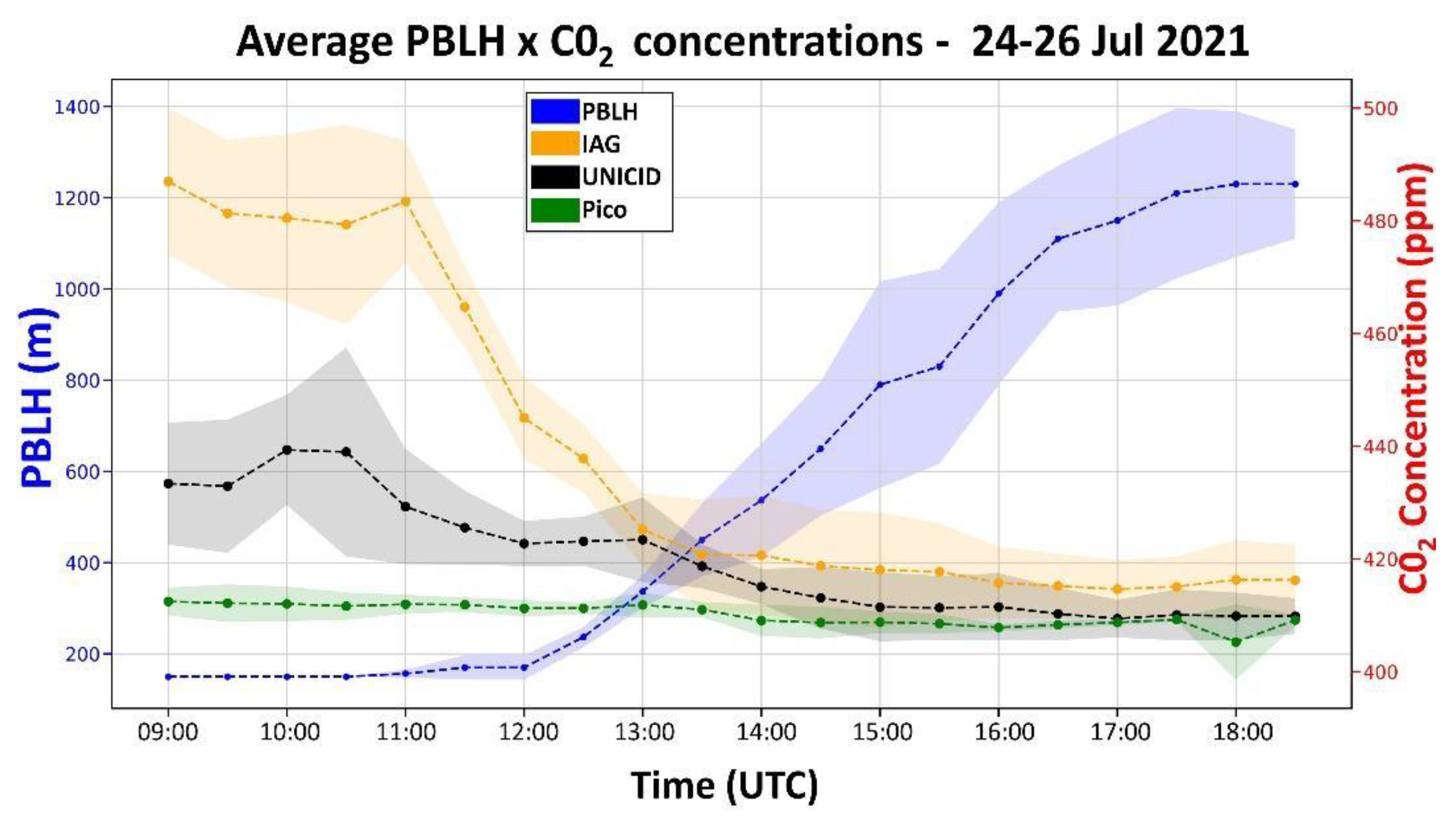
3.2. Case Study: CO2 and CH4 Concentrations in the Planetary Boundary Layer during 24–26 July 2021

Between 24 July and 26 July 2021, the weather conditions were devoid of substantial cloud cover. The absence of precipitation and cloud cover facilitated the acquisition of accurate PBL height retrievals for these specific days. Thus, this time frame was selected as a study case to investigate the observed alterations in PBLH during these three days and their correlation with changes in carbon dioxide and methane concentration values. PBLH data was obtained from the CIENTEC site, while CO2 and CH4 data were collected from the IAG, UNICID, and Pico do Jaraguá stations.
The range-corrected signal measured with the ceilometer on both 24 and 25 July, as well as the PBLH values retrieved using the WCT method for this period, are shown in Figure 6a,b.
The Single-Particle Lagrangian Integrated Trajectory Hybrid (HYSPLIT) model was developed by the NOAA Air Resources Laboratory; it is a system for calculating air mass trajectories as well as transport, dispersion, chemical transformation, and deposition simulations. The method of calculation of this model is a hybrid between the Lagrangian approach, using mobile reference data for advection and diffusion calculations as the trajectories of air masses move, and the Eulerian methodology which is based on calculating pollutant concentrations with a reference frame that uses a fixed three-dimensional grid method. It was used to verify the origin of the air masses that arrived in São Paulo during the analyzed period. The model was performed in backward trajectories of 24 h, due to the fact that the PBLH changes within this interval, and the selected hours were 9, 12, 15, 18, and 21 UTC in the locations of the three stations measuring the concentrations of CO2 and CH4. Analyzing the backward trajectories of air masses, as shown in Figure 7, it was noted that they come from the same region. One of the factors that would cause a high variation in the concentrations of CH4 and CO2 in the study area would be the transport of GHGs from regions with high methane production due to agriculture or plumes from fires. Both sources are mostly located further east, and such sources possibly were not located in the study region [44,45].

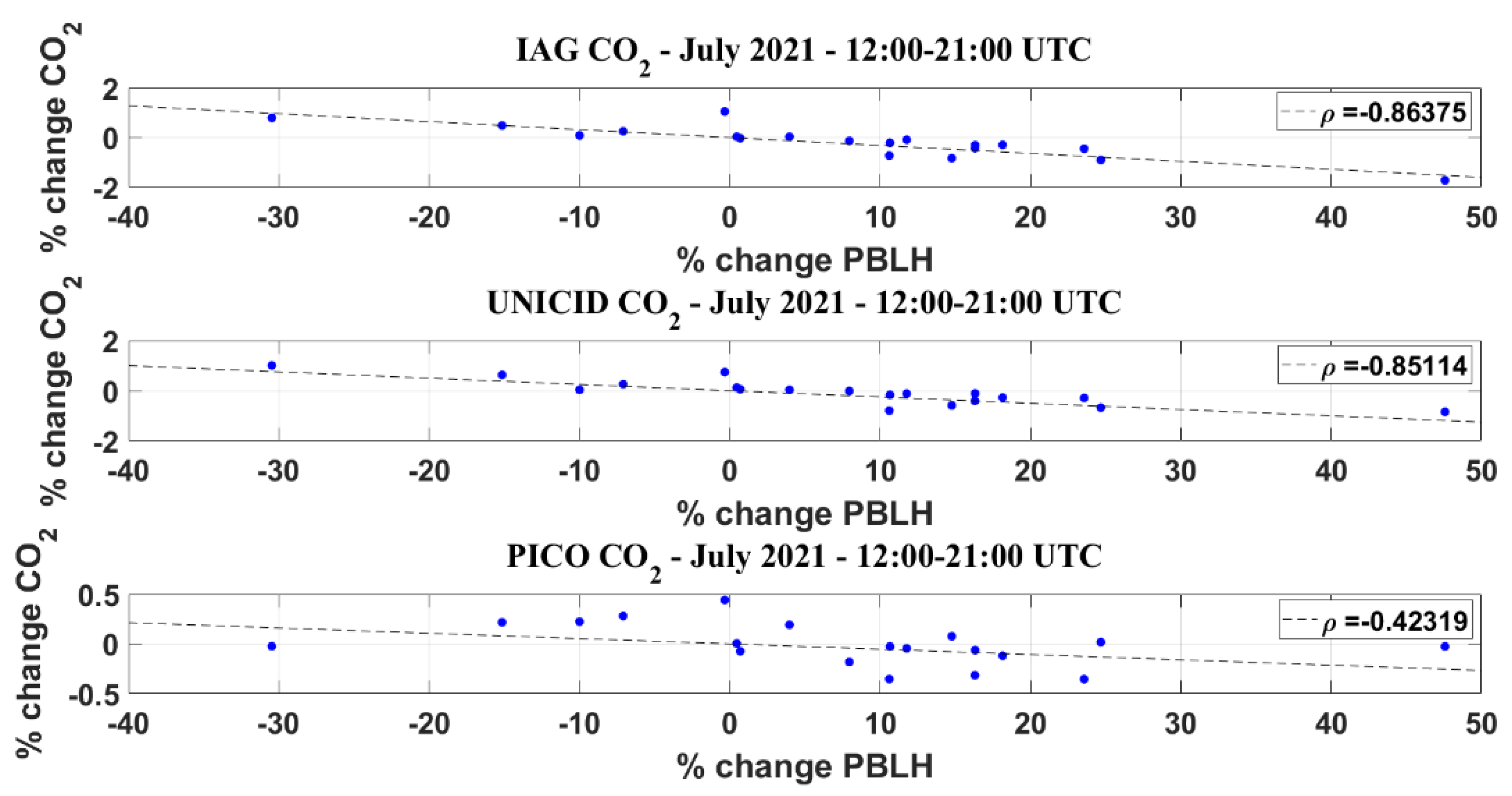
3.2.1. CO2 and CH4 Concentration Variations across Measuring Stations

Figure 8 presents the average PBLH obtained for the period spanning from 24 to 26 July 2021, as well as the average CO2 concentrations measured across the three stations. PBLHs and CH4 concentrations were also compared. Figure 9 shows the average PBLH heights obtained at CIENTEC and CH4 concentrations obtained at each site location. The shaded regions in Figure 8 and Figure 9 represent the standard deviations of values included in the averages.
An apparent inverse relationship or anticorrelation between PBLH and CO2 and CH4 concentrations can be seen in Figure 8 and Figure 9. This suggests that as the PBLH increases, CO2 and CH4 concentrations tend to decrease, indicating that lower PBL heights correspond to limited vertical mixing and the accumulation of these gases near the surface.
As can be seen in Figure 8 and Figure 9, there was a noticeable trend where both CO2 and CH4 concentrations at IAG and UNICID decrease as the PBLH increases. Generally, CO2 concentrations in urban areas are closely linked to local emissions and sinks. In the case of São Paulo, the primary sources of emissions are often associated with the large flow of vehicles. These concentrations can be affected by air mass transport and variations in the PBL [46]. GHGs emitted at ground level up to a certain height are well mixed in the planetary boundary layer [47]. The decrease in CO2 concentrations and increase in PBLH indicates that the height of the layer influences the dilution of the gas in question.
CH4 concentrations are predominantly regulated by sinks, with hydroxyl radical (OH) being the largest sink present in the atmosphere [48]. However, a similar behavior to that seen for CO2 can be observed concerning the relationship between the evolution of the boundary layer and methane concentrations. As the height of the PBL increases, there is a corresponding decrease in methane values. Even though methane is not categorized as a pollutant, previous studies such as Metya et al. (2021) [47] demonstrate that, throughout the day, the gases present in the lower troposphere are diluted as the boundary layer expands. CO2 and CH4 concentrations measured at the Pico do Jaraguá station did not follow the same pattern as seen at IAG and UNICID, due to the station’s location being the most distant from the city’s main emission sources.

3.2.2. Day-to-Day Variations

There were observed variations in the behavior of the PBLH throughout the three-day period, as seen in Figure 10. The maximum PBLH was similar across these three days, estimated at approximately 1290 m for 24 July, 1350 m for 25 July, and 1470 m for 26 July. PBL expansion occurred earlier each subsequent day, with PBL heights on 24 July being the most distinct, featuring an ascent that persisted until late afternoon. Changes in PBL heights during the afternoon were smaller on July 24, indicating a gradual but continuous increase in PBL heights and suggesting that, while PBL heights climbed more slowly on the 24th, the PBL continued to develop later into the afternoon than on the other days.
A similar trend was observed for the CO2 data, as shown in Figure 11a,b, as concentrations had a more pronounced decrease on 25 and 26 July than on 24 July. At the IAG station, CO2 concentrations reached minimum values of 410–415 ppm, while they remained above 420 ppm on 24 July. At the UNICID station, minimum CO2 concentrations of around 410 ppm were measured in the afternoons of 25 and 26 July, while on 24 July concentrations measured in the afternoon were roughly 10 ppm higher. The decrease in CH4 concentrations, as seen in the afternoon in Figure 11c,d, also shows a substantial difference in the values measured on July 24 when compared with those measured on 25 and 26 July: CH4 concentrations remained higher than the values measured on the 25th and 26th throughout most of the afternoon. While CH4 concentrations on the 25th and the 26th remained at around 2 ppm and 1.9 ppm at the IAG and UNICID sites, respectively, from 15:00 UTC until approximately 20:00 UTC, they gradually decreased during the afternoon on the 24th, eventually reaching values similar to those measured on the other two days.
The percentage changes in planetary boundary layer heights and in CO2 and CH4 concentrations at each measuring interval, that is, how much these values increased or decreased between successive 30 min data points, were derived from the data collected on 24–26 July 2021. Changes in PBL heights and CO2 and CH4 concentrations were compared and are shown in Figure 12 and Figure 13. The results revealed a pattern where negative changes (decreasing values) in PBL height were consistently associated with positive changes (increasing values) in CO2 and CH4 concentrations during the interval under investigation. Additionally, the results indicated that the majority of positive changes in PBL height were accompanied by negative changes in CO2 concentrations, with a few instances showing positive values near 0. To further understand the relationship between these variables, regression lines were fitted to the data. These regression lines demonstrated a negative correlation between CO2 and CH4 concentrations and PBL heights, passing near the origin point (0, 0). The correlation coefficient ρ was also obtained for each of the regression lines, with changes in PBL heights showing a correlation coefficient of −0.76 and −0.62 with CO2 concentrations at IAG and UNICID, respectively, and of −0.71 and −0.43 with CH4 concentrations at IAG and UNICID, respectively.

3.3. Monthly Averages

CO2 and CH4 concentrations exhibit variation between stations owing to the impact of local emissions and transport dynamics. Daily averages might not entirely capture the typical patterns observed at these monitoring stations, and distinctions in the average CO2 and CH4 concentrations among stations become more evident in longer-term measurements. In Figure 14, the monthly average PBL heights for July 2021 are presented, along with the average CO2 concentrations measured at the three stations. Only data from days without significant cloud cover were included. During July 2021, a total of 9 days displayed substantial cloud cover and were consequently excluded from the analysis. The average values for July 2021 were computed based on the data from the remaining 22 days.
The monthly averages provide a more distinct perspective regarding the contrast in CO2 concentrations across the three measurement stations. CO2 concentrations are highest at the IAG station and lowest at the Pico do Jaraguá station. At Pico do Jaraguá, average CO2 concentrations exhibit minimal diurnal variation, primarily due to its greater distance from local emission sources. IAG and UNICID display similar patterns in CO2 concentrations throughout the day. Peak average CO2 concentrations are reached at approximately 10:00–10:30 UTC, followed by a decline extending into mid-afternoon. A corresponding trend is observed in PBL heights, with the lowest average heights recorded in the early morning, followed by a swift rise from late morning until mid-afternoon.
Figure 15 shows the monthly average PBL heights and CH4 concentrations for July 2021.
Average CH4 concentrations exhibit a distinct pattern compared to average CO2 concentrations. At the IAG station, average CH4 concentrations peak at approximately 11:00–11:30 UTC and then decline rapidly until mid-afternoon. UNICID station shows higher values during the early morning and nighttime, with concentrations decreasing in the afternoon. The pattern for average CH4 concentrations measured at the Pico do Jaraguá station is less pronounced, with less variation in comparison to the other stations. However, average concentrations display more fluctuations during the morning and early afternoon, instead of a consistent decline.
The percentage change in PBL heights, as well as CO2 and CH4 concentrations at each measurement interval, were calculated for the data collected in the month of July and are shown in Figure 16 and Figure 17. Values were restricted to the timeframe spanning from 12:00 to 21:00 UTC, because during the late night and early morning hours PBLH values tend to decrease into the CHM 15k’s overlap range. Additionally, during nighttime, São Paulo experiences the influence of the sea breeze, which affects the city most days of the year [49,50], tending to trap aerosols within a lower layer of the PBL, which can lead to the WCT method falsely indicating a reduction in the PBLH.
Negative changes in CO2 and CH4 concentrations accompanied by concurrent positive changes in PBLH values indicate greater negative correlation between these variables. In Figure 16, we see more significant correlation between changes in CO2 concentrations and changes in PBLH values at the IAG station, with a ρ of approximately −0.86, and at the UNICID station, with a ρ of approximately −0.85, and less correlation at the Pico do Jaraguá station, with a ρ of approximately −0.42. The negative correlation between CH4 concentrations at IAG and PBLH values can be seen in Figure 17. This correlation is more significant for average values obtained from data measured at the IAG station, with a ρ of approximately −0.78, while the other stations show lower values with a ρ of −0.66 at UNICID and −0.38 at Pico do Jaraguá.

4. Conclusions

This work presented the results derived from the operation of a ceilometer during the month of July 2021. These ceilometer measurements were used to obtain the PBLHs with the wavelet covariance transform method. A lidar system also operated on 26 July 2021, and the PBLHs obtained with the WCT method using data from both instruments were subsequently compared. The comparison showed similar PBLHs at both locations, even though the instruments were positioned at two different locations in São Paulo roughly 15 km apart. Signal noise and attenuation may occur in the ceilometer’s data, but in clear sky conditions the instrument can still deliver accurate results. The PBLHs retrieved on 24–26 July 2021 were compared to the concentrations of CO2 and CH4 obtained in different locations in São Paulo in order to follow changes in the PBL related to the CO2 and CH4 concentrations. The ceilometer-retrieved PBL heights were also compared to the CO2 and CH4 concentrations at all the three MASP sites, as the PBL heights followed the changes in CO2 and CH4 with an opposite sign, i.e., increasing PBL heights corresponded to a decrease in CO2 and CH4 concentrations, showing a negative correlation between PBL heights versus concentrations (CO2 and CH4) throughout the day. The carbon dioxide and methane data also showed a correlation with PBL growth timing changes, with the highest PBL growth accompanied by decreased concentrations of carbon dioxide and methane.
Monthly average PBL heights and CO2 and CH4 concentrations were also obtained and compared for the month of July 2021. The average CO2 daily cycle for the month showed higher CH4 concentrations in the morning, which decreased rapidly in the late morning to early afternoon and then changed little until increasing again in the late afternoon and early evening. The average CH4 daily cycle for July 2021 showed a less clear pattern. CH4 concentrations were higher in the morning and decreased in the afternoon at all stations, but there was a significant difference in behavior between the stations for most of the day. Despite their different daily cycles, all stations showed similar average CH4 concentrations in mid-afternoon. The correlation between changes in average CO2 concentrations and PBLH values was also analyzed, showing higher correlation for the IAG and UNICID stations, with ρ correlation coefficients of approximately −0.86 and −0.85, respectively, and lower for Pico do Jaraguá, with a ρ of −0.42. When comparing changes in CH4 concentrations and changes in PBL height, these also showed negative correlation, with a correlation coefficient of approximately −0.78 for IAG, −0.66 for UNICID, and −0.38 for Pico do Jaraguá.
The results demonstrated that CO2 concentrations exhibited a more pronounced correlation with PBL heights than CH4 concentrations, as their behavior differed due to distinct sources and sinks. The results from this study contribute to advancing our understanding of the relationship between PBLH and greenhouse gas concentrations, and of the role of local emissions in shaping this relationship, as evidenced by the varying outcomes across the three measurement stations and by the daily variations in CO2/CH4 concentrations and PBLH values, while additionally highlighting the value of remote sensing instruments like ceilometers for tracking and studying atmospheric processes.

Author Contributions

Conceptualization, A.V.d.S. and E.L.; methodology, A.V.d.S.; software, A.V.d.S.; validation, A.V.d.S.; formal analysis, A.V.d.S. and E.L.; investigation, A.V.d.S., E.C.A., I.d.S.A., T.C. and F.d.M.M.; resources, E.L.; data curation, A.V.d.S., I.d.S.A., M.T.A.M., C.E.S.-O. and N.F.L.; writing—original draft preparation, A.V.d.S.; writing—review and editing, A.V.d.S., G.S., G.d.A.M., P.P.d.Q.L., E.C.A. and I.d.S.A.; visualization, A.V.d.S.; supervision, E.L.; project administration, E.L. and M.d.F.A.; funding acquisition, M.d.F.A. All authors have read and agreed to the published version of the manuscript.

Funding

This research was funded by the Brazilian Research Foundation (CAPES) (scholarships: 88887.473711/2020-00, 88887.464990/2019-00, 88887.511325/2020-00, 88887.473416/2020-00, 88887.859244/2023-00), the National Council for Scientific and Technological Development (CNPq), and the São Paulo Research Foundation (FAPESP): METROCLIMA project (process 2016/18438-0).

Institutional Review Board Statement

Not applicable.

Informed Consent Statement

Not applicable.

Data Availability Statement

No publicly archived datasets have been published yet.

Acknowledgments

We thank the Metroclima project for the support to the data acquisition (http://www.metroclima.iag.usp.br/, accessed on 15 October 2023), IPEN, FAPESP, CAPES, CNPq and Leal teams for their support throughout the measurement period. The authors gratefully acknowledge the NOAA Air Resources Laboratory (ARL) for the provision of the HYSPLIT transport and dispersion model and/or READY website (https://www.ready.noaa.gov, accessed on 20 October 2023) used in this publication.

Conflicts of Interest

The authors declare no conflict of interest.

References

  1. Stull, R.B. An Introduction to Boundary Layer Meteorology; Kluwer Academic Publishers: New York, NY, USA, 1988. [Google Scholar]
  2. Seibert, P.; Beyrich, F.; Gryning, S.-E.; Joffre, S.; Rasmussen, A.; Tercier, P. Review and intercomparison of operational methods for the determination of the mixing height. Atmos. Environ. 2000, 34, 1001–1027. [Google Scholar] [CrossRef]
  3. Medeiros, B.; Hall, A.; Stevens, B. What Controls the Mean Depth of the PBL? J. Clim. 2005, 18, 3157–3172. [Google Scholar] [CrossRef]
  4. Kim, J.; Verma, S.B. Carbon dioxide exchange in a temperate grassland ecosystem. Bound.-Layer Meteorol. 1990, 52, 135–149. [Google Scholar] [CrossRef]
  5. Jacobs, C.M.J.; De Bruin, H.A.R. The Sensitivity of Regional Transpiration to Land-Surface Characteristics: Significance of Feedback. J. Clim. 1992, 5, 683–698. [Google Scholar] [CrossRef]
  6. Moreira, G.d.A.; Guerrero-Rascado, J.L.; Bravo-Aranda, J.A.; Benavent-Oltra, J.A.; Ortiz-Amezcua, P.; Róman, R.; Bedoya-Velásquez, A.E.; Landulfo, E.; Alados-Arboledas, L. Study of the planetary boundary layer by microwave radiometer, elastic lidar and Doppler lidar estimations in Southern Iberian Peninsula. Atmos. Res. 2018, 213, 185–195. [Google Scholar] [CrossRef]
  7. Cohn, S.A.; Angevine, W.M. Boundary layer height and entrainment zone thickness measured by lidars and wind-profiling radars. J. Applied. Meteorol. 2000, 39, 1233–1247. [Google Scholar] [CrossRef]
  8. Cimini, D.; De Angelis, F.; Dupont, J.-C.; Pal, S.; Haeffelin, M. Mixing layer height retrievals by multichannel microwave radiometer observations. Atmos. Meas. Tech. 2013, 6, 2941–2951. [Google Scholar] [CrossRef]
  9. Menut, L.; Flamant, C.; Pelon, J.; Flamant, P.H. Urban boundary-layer height determination from lidar measurements over the Paris area. Appl. Opt. 1999, 38, 945–954. [Google Scholar] [CrossRef]
  10. Moreira, G.d.A.; Guerrero-Rascado, J.L.; Benavent-Oltra, J.A.; Ortiz-Amezcua, P.; Román, R.; Bedoya-Velásquez, A.E.; Bravo-Aranda, J.A.; Reyes, F.J.O.; Landulfo, E.; Alados-Arboledas, L. Analyzing the turbulent planetary boundary layer by remote sensing systems: The Doppler wind lidar, aerosol elastic lidar and microwave radiometer. Atmos. Meas. Tech. 2019, 19, 1263–1280. [Google Scholar] [CrossRef]
  11. Liu, B.; Ma, Y.; Gong, W.; Zhang, M.; Yang, J. Improved two-wavelength Lidar algorithm for retrieving atmospheric boundary layer height. J. Quant. Spectrosc. Radiat. Transf. 2018, 224, 55–61. [Google Scholar] [CrossRef]
  12. Davis, K.J.; Gamage, N.; Hagelberg, C.R.; Kiemle, C.; Lenschow, D.H.; Sullivan, P.P. An Objective Method for Deriving Atmospheric Structure from Airborne Lidar Observations. J. Atmos. Ocean. Technol. 2000, 17, 1455–1468. [Google Scholar] [CrossRef]
  13. Li, H.; Yang, Y.; Hu, X.; Huang, Z.; Wang, G.; Zhang, B.; Zhang, T. Evaluation of retrieval methods of daytime convective boundary layer height based on lidar data. J. Geophys. Res. Atmos. 2017, 122, 4578–4593. [Google Scholar] [CrossRef]
  14. Weitkamp, C. Lidar: Range-Resolved Optical Remote Sensing of the Atmosphere. In Springer Series in Optical Sciences; Springer: New York, NY, USA, 2005; Volume 102. [Google Scholar]
  15. Kovalev, V.A.; Eichinger, W.E. Elastic Lidar: Theory, Practice, and Analysis Methods; John Wiley & Sons: Hoboken, NJ, USA, 2004. [Google Scholar]
  16. Baars, H.; Ansmann, A.; Engelmann, R.; Althausen, D. Continuous monitoring of the boundary-layer top with lidar. Atmos. Meas. Tech. 2008, 8, 7281–7296. [Google Scholar] [CrossRef]
  17. Martucci, G.; Matthey, R.; Mitev, V.; Richner, H. Comparison between Backscatter Lidar and Radiosonde Measurements of the Diurnal and Nocturnal Stratification in the Lower Troposphere. J. Atmos. Ocean. Technol. 2007, 24, 1231–1244. [Google Scholar] [CrossRef]
  18. Granados-Muñoz, M.J.; Navas-Guzmán, F.; Bravo-Aranda, J.A.; Guerrero-Rascado, J.L.; Lyamani, H.; Fernández-Gálvez, J.; Alados-Arboledas, L. Automatic determination of the planetary boundary layer height using lidar: One-year analysis over southeastern Spain. J. Geophys. Res. Atmos. 2012, 117, D18208. [Google Scholar] [CrossRef]
  19. Moreira, G.d.A.; Lopes, F.J.d.S.; Guerrero-Rascado, J.L.; Granados-Muñoz, M.J.; Bourayou, R.; Landulfo, E. Comparison between two algorithms based on different wavelets to obtain the Planetary Boundary Layer height. In Proceedings of the SPIE 9246, Lidar Technologies, Techniques, and Measurements for Atmospheric Remote Sensing, 92460H, Ottawa, ON, USA, 18 November 2014; p. 92460D. [Google Scholar]
  20. Pal, S.; Behrendt, A.; Wulfmeyer, V. Elastic-backscatter-lidar-based characterization of the convective boundary layer and investigation of related statistics. Ann. Geophys. 2010, 28, 825–847. [Google Scholar] [CrossRef]
  21. Hooper, W.P.; Eloranta, E.W. Lidar measurements of wind in the planetary boundary layer: The method, accuracy, and results from joint measurements with radiosonde and kytoon. J. Appl. Meteorol. Climatol. 1986, 25, 990–1001. [Google Scholar] [CrossRef]
  22. Piironen, A.K.; Eloranta, E.W. Convective boundary layer mean depths and cloud geometrical properties obtained from volume imaging lidar data. J. Geophys. Res. Atmos. 1995, 100, 25569–25576. [Google Scholar] [CrossRef]
  23. Hayden, K.; Anlauf, K.; Hoff, R.; Strapp, J.; Bottenheim, J.; Wiebe, H.; Froude, F.; Martin, J.; Steyn, D.; McKendry, I. The vertical chemical and meteorological structure of the boundary layer in the Lower Fraser Valley during Pacific’93. Atmos. Environ. 1997, 31, 2089–2105. [Google Scholar] [CrossRef]
  24. De Bruine, M.; Apituley, A.; Donovan, D.P.; Baltink, H.K.; de Haij, M.J. Pathfinder: Applying graph theory to consistent tracking of daytime mixed layer height with backscatter lidar. Atmos. Meas. Tech. 2017, 10, 1893–1909. [Google Scholar] [CrossRef]
  25. Caicedo, V.; Rappenglück, B.; Lefer, B.; Morris, G.; Toledo, D.; Delgado, R. Comparison of aerosol lidar retrieval methods for boundary layer height detection using ceilometer aerosol backscatter data. Atmos. Meas. Tech. 2017, 10, 1609–1622. [Google Scholar] [CrossRef]
  26. Brooks, I.M. Finding Boundary Layer Top: Application of a Wavelet Covariance Transform to Lidar Backscatter Profiles. J. Atmos. Ocean. Technol. 2003, 20, 1092–1105. [Google Scholar] [CrossRef]
  27. Uzan, L.; Egert, S.; Alpert, P. Ceilometer evaluation of the eastern Mediterranean summer boundary layer height—First study of two Israeli sites. Atmos. Meas. Tech. 2016, 9, 4387–4398. [Google Scholar] [CrossRef]
  28. Steyn, D.G.; Baldi, M.; Hoff, R. The Detection of Mixed Layer Depth and Entrainment Zone Thickness from Lidar Backscatter Profiles. J. Atmos. Oceanic Technol. 1999, 16, 953–959. [Google Scholar] [CrossRef]
  29. Eresmaa, N.; Karppinen, A.; Joffre, S.M.; Räsänen, J.; Talvitie, H. Mixing height determination by ceilometer. Atmos. Meas. Tech. 2006, 6, 1485–1493. [Google Scholar] [CrossRef]
  30. Haeffelin, M.; Angelini, F.; Morille, Y.; Martucci, G.; Frey, S.; Gobbi, G.P.; Lolli, S.; O’dowd, C.D.; Sauvage, L.; Xueref-Rémy, I.; et al. Evaluation of Mixing-Height Retrievals from Automatic Profiling Lidars and Ceilometers in View of Future Integrated Networks in Europe. Boundary-Layer Meteorol. 2012, 143, 49–75. [Google Scholar] [CrossRef]
  31. Culf, A.; Fisch, G.; Malhi, Y.; Nobre, C. The influence of the atmospheric boundary layer on carbon dioxide concentrations over a tropical forest. Agric. For. Meteorol. 1997, 85, 149–158. [Google Scholar] [CrossRef]
  32. Carvalho, V.S.B.; Freitas, E.D.; Martins, L.D.; Martins, J.A.; Mazzoli, C.R.; Andrade, M.d.F. Air quality status and trends over the Metropolitan Area of São Paulo, Brazil as a result of emission control policies. Environ. Sci. Policy 2015, 47, 68–79. [Google Scholar] [CrossRef]
  33. Ballantyne, A.P.; Alden, C.B.; Miller, J.B.; Tans, P.P.; White, J.W.C. Increase in observed net carbon dioxide uptake by land and oceans during the past 50 years. Nature 2012, 488, 70–72. [Google Scholar] [CrossRef]
  34. Hodnebrog, O.; Aamaas, B.; Fuglestvedt, J.S.; Marston, G.; Myhre, G.; Nielsen, C.J.; Sandstad, M.; Shine, K.P.; Wallington, T.J. Updated Global Warming Potentials and Radiative Efficiencies of Halocarbons and Other Weak Atmospheric Absorbers. Rev. Geophys. 2020, 58, e2019RG000691. [Google Scholar] [CrossRef]
  35. IPCC; Masson-Delmotte, V.; Zhai, P.; Pirani, A.; Connors, S.L.; Péan, C.; Berger, S.; Caud, N.; Chen, Y.; Goldfarb, L.; et al. Climate Change 2021: The Physical Science Basis. In Contribution of Working Group I to the Sixth Assessment Report of the Intergovernmental Panel on Climate Change; Cambridge University Press: Cambridge, UK; New York, NY, USA, 2021; pp. 3–32. [Google Scholar]
  36. WMO. The State of Greenhouse Gases in the Atmosphere Based on Global Observations through 2020. In Greenhouse Gas Bulletin (GHG Bulletin); WMO: Geneva, Switzerland, 2021; Volume 17, p. 67. [Google Scholar]
  37. Ramanathan, V.; Cicerone, R.J.; Singh, H.B.; Kiehl, J.T. Trace gas trends and their potential role in climate change. J. Geophys. Res. 1985, 90, 5547–5566. [Google Scholar] [CrossRef]
  38. Myhre, G.; Samset, B.H.; Schulz, M.; Balkanski, Y.; Bauer, S.; Berntsen, T.K.; Bian, H.; Bellouin, N.; Chin, M.; Diehl, T.; et al. Radiative forcing of the direct aerosol effect from AeroCom Phase II simulations. Atmos. Meas. Tech. 2013, 13, 1853–1877. [Google Scholar] [CrossRef]
  39. Canadell, J.G.; Ciais, P.; Dhakal, S.; Dolman, H.; Friedlingstein, P.; Gurney, K.R.; Held, A.; Jackson, R.B.; Le Quéré, C.; Malone, E.L.; et al. Interactions of the carbon cycle, human activity, and the climate system: A research portfolio. Curr. Opin. Environ. Sustain. 2010, 2, 301–311. [Google Scholar] [CrossRef]
  40. IBGE—Instituto Brasileiro de Geografia e Estatística Home Page. Available online: http://ibge.gov.br (accessed on 24 February 2023).
  41. De Oliveira, A.P.; Filho, E.P.M.; Ferreira, M.J.; Codato, G.; Ribeiro, F.N.D.; Landulfo, E.; Moreira, G.d.A.; Pereira, M.M.R.; Mlakar, P.; Boznar, M.Z.; et al. Assessing Urban Effects on the Elimate of Metropolitan Regions Of Brazil—Preliminary Results of the MCITY BRAZIL Project. Explor. Environ. Sci. Res. 2020, 1, 38–77. [Google Scholar] [CrossRef]
  42. Tang, G.; Zhang, J.; Zhu, X.; Song, T.; Münkel, C.; Hu, B.; Schäfer, K.; Liu, Z.; Zhang, J.; Wang, L.; et al. Mixing layer height and its implications for air pollution over Beijing, China. Atmos. Meas. Tech. 2016, 16, 2459–2475. [Google Scholar] [CrossRef]
  43. Moreira, G.d.A.; de Oliveira, A.P.; Codato, G.; Sánchez, M.P.; Tito, J.V.; e Silva, L.A.H.; da Silveira, L.C.; da Silva, J.J.; Lopes, F.J.d.S.; Landulfo, E. Assessing Spatial Variation of PBL Height and Aerosol Layer Aloft in São Paulo Megacity Using Simul-taneously Two Lidar during Winter 2019. Atmosphere 2022, 13, 611. [Google Scholar] [CrossRef]
  44. Stein, A.F.; Draxler, R.R.; Rolph, G.D.; Stunder, B.J.B.; Cohen, M.D.; Ngan, F. NOAA’s HYSPLIT Atmospheric Transport and Dispersion Modeling System. Bull. Am. Meteorol. Soc. 2015, 96, 2059–2077. [Google Scholar] [CrossRef]
  45. Rolph, G.; Stein, A.; Stunder, B. Real-time Environmental Applications and Display sYstem: READY. Environ. Model. Softw. 2017, 95, 210–228. [Google Scholar] [CrossRef]
  46. Wang, P.; Zhou, W.; Niu, Z.; Xiong, X.; Wu, S.; Cheng, P.; Hou, Y.; Lu, X.; Du, H. Spatio-temporal variability of atmospheric CO2 and its main causes: A case study in Xi’an city, China. Atmos. Res. 2021, 249, 105346. [Google Scholar] [CrossRef]
  47. Metya, A.; Datye, A.; Chakraborty, S.; Tiwari, Y.K.; Sarma, D.; Bora, A.; Gogoi, N. Diurnal and seasonal variability of CO2 and CH4 concentration in a semi-urban environment of western India. Sci. Rep. 2021, 11, 1–13. [Google Scholar] [CrossRef]
  48. Vaghjiani, G.L.; Ravishankara, A. New measurement of the rate coefficient for the reaction of OH with methane. Nature 1991, 350, 406–409. [Google Scholar] [CrossRef]
  49. Oliveira, A.P.; Bornstein, R.D.; Soares, J. Annual and Diurnal Wind Patterns in the City of São Paulo. Water Air Soil Pollut. 2003, 3, 3–15. [Google Scholar] [CrossRef]
  50. Lolli, S. Machine Learning Techniques for Vertical Lidar-Based Detection, Characterization, and Classification of Aerosols and Clouds: A Comprehensive Survey. Remote. Sens. 2023, 15, 4318. [Google Scholar] [CrossRef]
Figure 1. (a) CHM 15k ceilometer and (b) MSP1 lidar.
Atmosphere 14 01830 g001
Figure 2. Locations of and distances between the IPEN and CIENTEC stations, IAG, UNICID, and Pico do Jaraguá stations. Scale 1:200,000. https://geoone.com.br/mapas-qgis/ (accessed on 14 October 2023). Using: QGIS (GIS software). Version 3.28.11. QGIS Geographic Information System. Open Source Geospatial Foundation Project. http://qgis.osgeo.org, (accessed on 4 September 2023).
Atmosphere 14 01830 g002
Figure 3. Representation of the Haar function.
Atmosphere 14 01830 g003
Figure 4. Diurnal evolution of PBLH at (a) CIENTEC and (b) IPEN on 26 July 2021.
Atmosphere 14 01830 g004
Figure 5. Black line is the height difference between PBLHs obtained with lidar and ceilometer data and blue line is PBLHs retrieved at IPEN and red line CIENTEC on 26 July 2021.
Atmosphere 14 01830 g005
Figure 6. Diurnal evolution of PBLH at CIENTEC on (a) 24 July 2021, (b) 25 July 2021.
Atmosphere 14 01830 g006
Figure 7. Back trajectories from HYSPLIT at inlet heights on 24th to 26th July are displayed for three locations: IAG at 15 m (ac), UNICID at 38 m (df), and Pico do Jaraguá at 3 m (gi). Trajectories are color-coded by arrival time: pink curves depict trajectories arriving at 9 UTC, cyan curves at 12 UTC, green curves at 15 UTC, blue curves at 18 UTC, and orange curves at 21 UTC.
Atmosphere 14 01830 g007
Figure 8. Average PBLH and CO2 concentrations from 24 July to 26 July 2021.
Atmosphere 14 01830 g008
Figure 9. Average PBLH and CH4 concentrations from 24 July to 26 July 2021.
Atmosphere 14 01830 g009
Figure 10. Average planetary boundary layer heights obtained on 24 July 2021 (yellow solid line), 25 July 2021 (black solid line), and 26 July 2021 (green solid line). Standard deviations are represented by the shaded regions.
Atmosphere 14 01830 g010
Figure 11. Average concentrations of CO2 at (a) IAG and (b) UNICID, and of CH4 at (c) IAG and (d) UNICID.
Atmosphere 14 01830 g011
Figure 12. Scatter plots of percentage differences in CO2 concentrations at IAG and UNICID, and in PBL heights. Each data point corresponds to CO2 and PBLH values obtained every 30 min from 10:30 to 20:00 UTC on 24 July 2021 (in blue), 25 July 2021 (in red), and 25 July 2021 (in black). The dashed black lines show the regression lines fit to these data points. The correlation coefficient ρ calculated for each station is also shown.
Atmosphere 14 01830 g012
Figure 13. Scatter plots of percentage differences in CH4 concentrations at IAG and UNICID, and in PBL heights. Each data point corresponds to CH4 and PBLH values obtained every 30 min from 10:30 to 20:00 UTC on 24 July 2021 (in blue), 25 July 2021 (in red), and 25 July 2021 (in black). The dashed black lines show the regression lines fit to these data points. The correlation coefficient ρ calculated for each station is also shown.
Atmosphere 14 01830 g013
Figure 14. Average PBLH and CO2 concentrations for July 2021.
Atmosphere 14 01830 g014
Figure 15. Average PBLH and CH4 concentrations for July 2021.
Atmosphere 14 01830 g015
Figure 16. Scatter plots of percentage differences in CO2 concentrations at IAG, UNICID, and Pico do Jaraguá, and in PBL heights. Each data point corresponds to the average CO2 and PBLH values obtained every 30 min from 12:00 to 21:00 UTC in July 2021. The dashed black lines show the regression lines fit to these data points. The correlation coefficients ρ are also shown.
Atmosphere 14 01830 g016
Figure 17. Scatter plots of percentage differences in CH4 concentrations at IAG, UNICID, and Pico do Jaraguá, and in PBL heights. Each data point corresponds to the average CH4 and PBLH values obtained every 30 min from 12:00 to 21:00 UTC in July 2021. The dashed black lines show the regression lines fit to these data points. The correlation coefficient ρ are also shown.
Atmosphere 14 01830 g017
Table 1. CO2 and CH4 monitoring site details and instrument models at each location.
Site NameInlet Height (m agl)Site Elevation
(m asl)
LatitudeLongitudeAnalyzerMeasuring
IAG15731−23.55947−46.733533G2301 IICO2, CH4
UNICID38741−23.53586−46.559550G2401CO, CO2, CH4
Pico do Jaraguá31079−23.45631−46.766094G2301-mCO2, CH4
Disclaimer/Publisher’s Note: The statements, opinions and data contained in all publications are solely those of the individual author(s) and contributor(s) and not of MDPI and/or the editor(s). MDPI and/or the editor(s) disclaim responsibility for any injury to people or property resulting from any ideas, methods, instructions or products referred to in the content.

