Stratospheric Warming Events in the Period January–March 2023 and Their Impact on Stratospheric Ozone in the Northern Hemisphere

Abstract

In this investigation, a comparison is presented between variations in temperature and ozone concentration at different altitude levels in the stratosphere for the Northern Hemisphere in the conditions of Sudden Stratospheric Warming (SSW) for the period January–March 2023. Spatial and altitude distribution of atmospheric characteristics derived from MERRA-2 are represented by their Fourier decomposition. A cross-correlation analysis between temperature and Total Ozone Column (TOC) is used. The longitudinal inhomogeneities in temperature, caused by stationary Planetary Waves with wavenumber 1 (SPW1), are found to be significant at altitudes around the maximum of the maximum of the ozone number density vertical distribution. As a result, it is established that the latitudinal and longitudinal distribution of TOC has a noticeable similarity with that of the temperature at altitudes close to the ozone concentration maximum. The results of correlation between temperature at individual stratospheric levels and ozone concentration show that (i) in the region around the ozone concentration maximum, the correlation is high and positive, (ii) at higher altitudes the sign of the correlation changes to negative (~37 km). The examination shows that the anomalous increases in TOC during SSW are due to an increase in ozone concentration in the altitudes between 10 km and 15 km.

1. Introduction

The role of ozone as a trace gas in the atmosphere is well known to scientists working in this field [1]. In general, the ozone located at different altitudes can be seen as beneficial, but also as harmful to life on planet Earth [2]. On the one hand, stratospheric ozone plays a protective role for the biosphere, due to the absorption of solar UV radiation, on the other hand, tropospheric ozone, being a pollutant, is harmful to human health [3,4]. Global amounts of ozone reached their minimum at the end of the last century when the Antarctic ozone hole was discovered [5]. In order to introduce measures against the chemical reactions leading to the destruction of the ozone, the Montreal Protocol was signed [6]. The results of this protocol are associated with a decrease in concentrations of ozone-depleting substances [7]. After the signing of the protocol, great importance is given to the effects of climate change on the stratospheric ozone and the impact of increasing greenhouse gases on the ‘‘recovery’’ process of the stratospheric ozone [8,9,10,11].

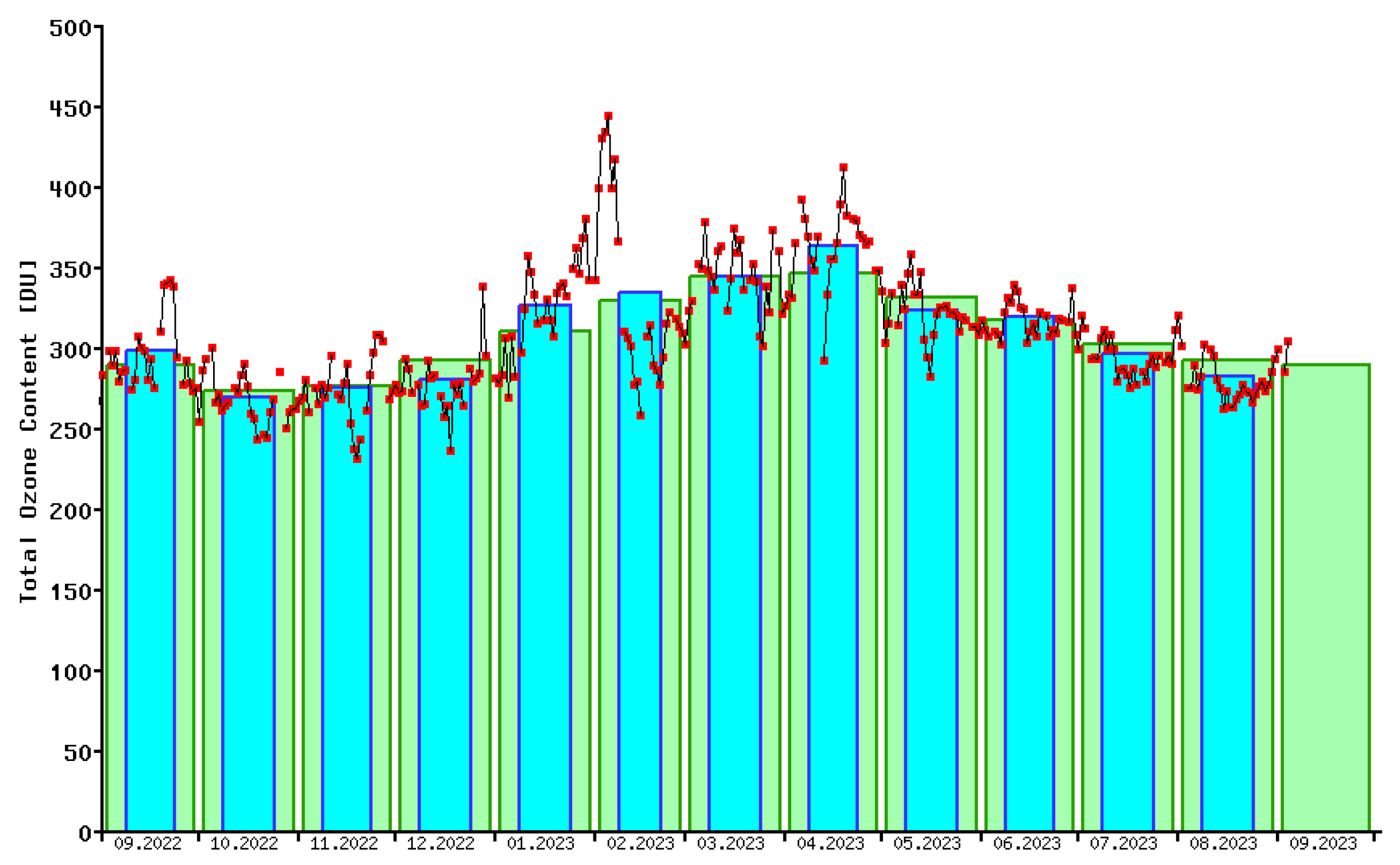
The idea for the present study is related to the TOC anomaly over Sofia observed in February 2023 through the equipment of the National Institute of Geophysics, Geodesy, and Geography at the Bulgarian Academy of Sciences—NIGGG, BAS (data are available at: http://www.geophys.bas.bg/total_ozone/total_ozone_en.htm, accessed on 27 November 2023). As can be seen in Figure 1 showing the NIGGG data, the extremely high TOC value (about 450 DU) at the beginning of the month of February is replaced by a significantly low value for the season in the middle of the month (up to about 250 DU). The TOC variation reaches up to 200 DU. Some studies of long-term variations of the protective ozone layer at mid-latitudes in the Northern Hemisphere and in particular over Bulgaria in recent decades show that it is relatively stable, with no significant trends being observed [2,12]. It is well known that the strongest short-term variations in ozone concentration and total stratospheric ozone are observed during the winter seasons, especially during Sudden Stratospheric Warming [13].

Stratospheric warmings are large-scale anomalies in the winter regime of the stratosphere which cause strong variations in temperature, pressure, and wind speed without any external factor being identified for their occurrence and without the presence of any additional energy into the stratosphere [14]. Stratospheric warming is caused by baric inhomogeneities with origin mainly in the troposphere, which, in the form of Stationary Planetary Waves (SPW), propagate vertically upwards with an increase in their amplitude, causing a destruction of the polar vortex in the polar regions [15]. The result is a reversal of the direction of the stratospheric zonal mean wind from a positive direction, which is normal for the winter season, to a negative direction [16]. When the wind reversal at 60° N reaches the 10 hPa level, the stratospheric warming is classified as major, whereas in other cases, according to the classifications, it is minor [16,17]. The disruption of polar vortex creates conditions for the penetration of warm air from low latitudes to push into the regions near the pole, causing a significant increase in polar stratospheric temperature, which is one of the important manifestations of SSW. A relevant aspect of SSWs, which is relevant for surface climate predictability, is the dynamical coupling between the stratosphere and troposphere [18].

The area of the stratosphere in which the strongest variations in atmospheric characteristics (temperature, pressure, and wind) are observed is approximately between 30 and 50 km. The present study, which aims to investigate variations in the stratospheric ozone, focuses on the behavior of the stratosphere between the tropopause (about 11 km) and 30 km of altitude, where the main mass of stratospheric ozone is concentrated, forming the value TOC, which is the most representative characteristic of the protective properties of stratospheric ozone.

Some studies show that in the altitudinal range of significant ozone concentration, variations in it and in TOC are caused by dynamical factors due to the fact that in this region of the stratosphere the lifetime of ozone is significant [19]. What the lifetime is of ozone is an interesting and detailed question researched scientists. According to some studies “the lifetime of an ozone molecule is still of the order of a year” [20]. Findings from additional studies concerning the height-dependent chemical loss lifetime reveal that in tropical regions, the chemical loss lifetime exceeds 100 times the advective lifetime at 70 hPa. The resulting lifetime at 20–30 hPa, which is 10 times shorter than the advective timescale at 10 hPa, is to the order of 100–200 days [21].

In turn, the dynamics of the stratosphere is determined by the spatial distribution of temperature and pressure.

The relationship between ozone concentration and temperature in the lower stratosphere is primarily characterized by a positive dependence, driven by the temperature-related increase in the destruction of ozone molecules through chemical reactions. The positive correlation in the dynamically controlled region is not as obvious, since it depends on the correlation between the ozone and the meridional and vertical winds’ wave perturbations, as well as on the vertical and meridional gradients of zonal mean ozone [22]. At the upper stratosphere, the temperature dependence of photochemical reactions prevails, and it turns out to be negative [23]. Due to the fact that the main mass of ozone is concentrated in the lower stratosphere, TOC is expected to have a positive correlation with temperature in the lower stratosphere. During the winter season, these stratospheric characteristics have much greater variability, which is due to the excitation of Planetary Waves that propagate in the stratosphere during the whole winter season, which is the main reason for the increased variability of the ozone layer in winter.

Dynamic control of ozone concentration is associated with planetary wave coupling. In their study, Lubis et al. [24] discussed comprehensively that during the Northern Hemisphere winter, the enhanced wave reflection in the Arctic polar stratosphere due to strong polar vortex events can lead to reduced ozone concentration during early and midwinter and increased springtime ozone loss in late winter through heterogeneous chemical processes. In contrast, winter dominated by SSWs leads to an increase in ozone concentration during early and midwinter due to stronger residual circulation and additional evidence is shown by [25].

For this reason, the present study was performed not only for the period of stratospheric warming, but for the entire 3-month period from January to March 2023, which made it possible to obtain reliable correlations between temperature and ozone concentration at different altitude levels in the stratosphere. The presence of a positive correlation between temperature and ozone has been established by some other studies [26,27]. This investigation attempts to confirm and clarify these results using global data. The detailed analysis presented allows tracing the well-known anomalies in TOC under SSW conditions.

2. Data and Methods

In the present research, the data from the measuring equipment of NIGGG-BAS were used. The measurements are performed with the sun photometer Microtops II, a production of Solar Light Company, USA (more information can be found on the official website of the producer: https://solarlight.com/microtops-ii-sunphotometer/, accessed on 27 November 2023) [28]. When measurements cannot be taken due to cloudy weather, the data are filled with satellite data from the OMI, located on the AURA orbiting satellite in 2004 available online at https://Ozonewatch.gsfc.nasa.gov/data/omi/, accessed on 28 November 2023. The resulting time series should be considered free of systematic bias [12].

The analysis of the spatial and altitudinal distribution of stratospheric ozone is based on the assimilated data from MERRA2—Global Modeling and Assimilation Office (GMAO) [29,30,31].

These data are available at https://gmao.gsfc.nasa.gov/reanalysis/MERRA-2/, accessed on 26 November 2023. The data are averaged on a 2° × 2° grid. Ozone concentration was converted from ozone mixing ratio (kg/kg) to ozone mass concentration (mg/m³). In addition, TOC was calculated from the data by integrating the ozone profile from the Earth’s surface to the highest data level of 0.1 hPa. In this paper, the conversion of isobaric levels to altitudes is used according to the following formula:

$$h\left[km\right]=-7\ast \ln \left(P\right[hPa]/1013.0)$$

(1)

where P is the pressure at the corresponding isobaric level in hPa.

The paper uses the representation of the longitudinal distribution of atmospheric characteristics (temperature, geopotential, ozone concentration) by its Fourier series decomposition using the following formula:

$$\begin{gathered} V\left(lon,lat\right)=V_0\left(lat\right) \\ +{\sum }_{k=1}^2{V}_k(lat)cos\left(k\frac{2\pi }{360}lon-{\phi }_k\left(lat\right)\right)+N\left(lat\right) \end{gathered}$$

(2)

For each latitude and for each day, the values of the constant, amplitudes, and phases of the components with wavenumbers 1 and 2 are determined by the least squares method. The N term includes all other longitudinal variations that are not the subject of the present study. The components with wavenumbers 1 and 2 represent the so-called Stationary Planetary Waves (SPW1 and SPW2).

In this paper, a cross-correlation analysis between temperature and ozone concentration is used to show the existing causal relationship between these quantities [32,33].

3. Results

This section presents the changes in stratospheric characteristics for the considered period January–March 2023. In order to obtain a detailed view of SPW1 and SPW2, the amplitudes and phases of the 60° N stationary waves are shown. A comparison between the distribution of temperature and TOC at the 70 hPa level is illustrated. The latitudinal distribution of SPW1 and SPW2 stationary wave amplitudes in temperature and TOC at the 70 hPa level are also presented. A comparison between temperature and TOC at 70 hPa is presented and a correlation coefficient by zero-time lag between the two parameters is derived for the Northern Hemisphere. Various comparisons between temperature and TOC for individual points and levels are shown.

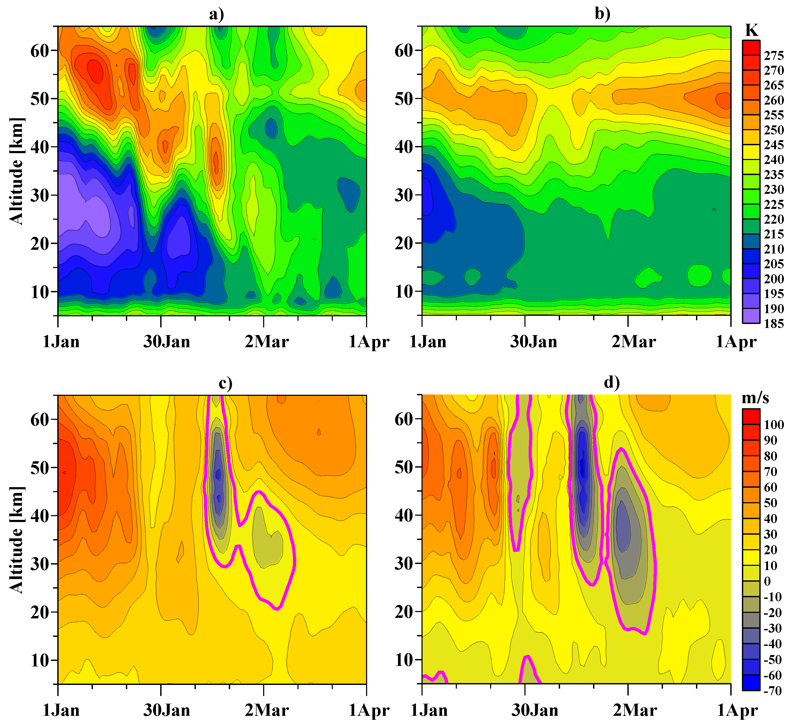
The behaviors shown in Figure 2 for some main characteristics of the stratosphere determine stratospheric warming in February, when at 60° N the direction of the zonal mean wind changes to 10 hPa (about 32 km). By definition, this stratospheric warming is major [16]. The poleward temperature increase and zonal wind reversion coincide in time with the TOC anomaly shown in Figure 1. The figure shows that, in addition to the major stratospheric warming in February, there is a significant increase in poleward temperature in late January and a reversal in zonal wind speed, which is observed at 70° N but absent at 60° N. This stratospheric warming can be classified as minor.

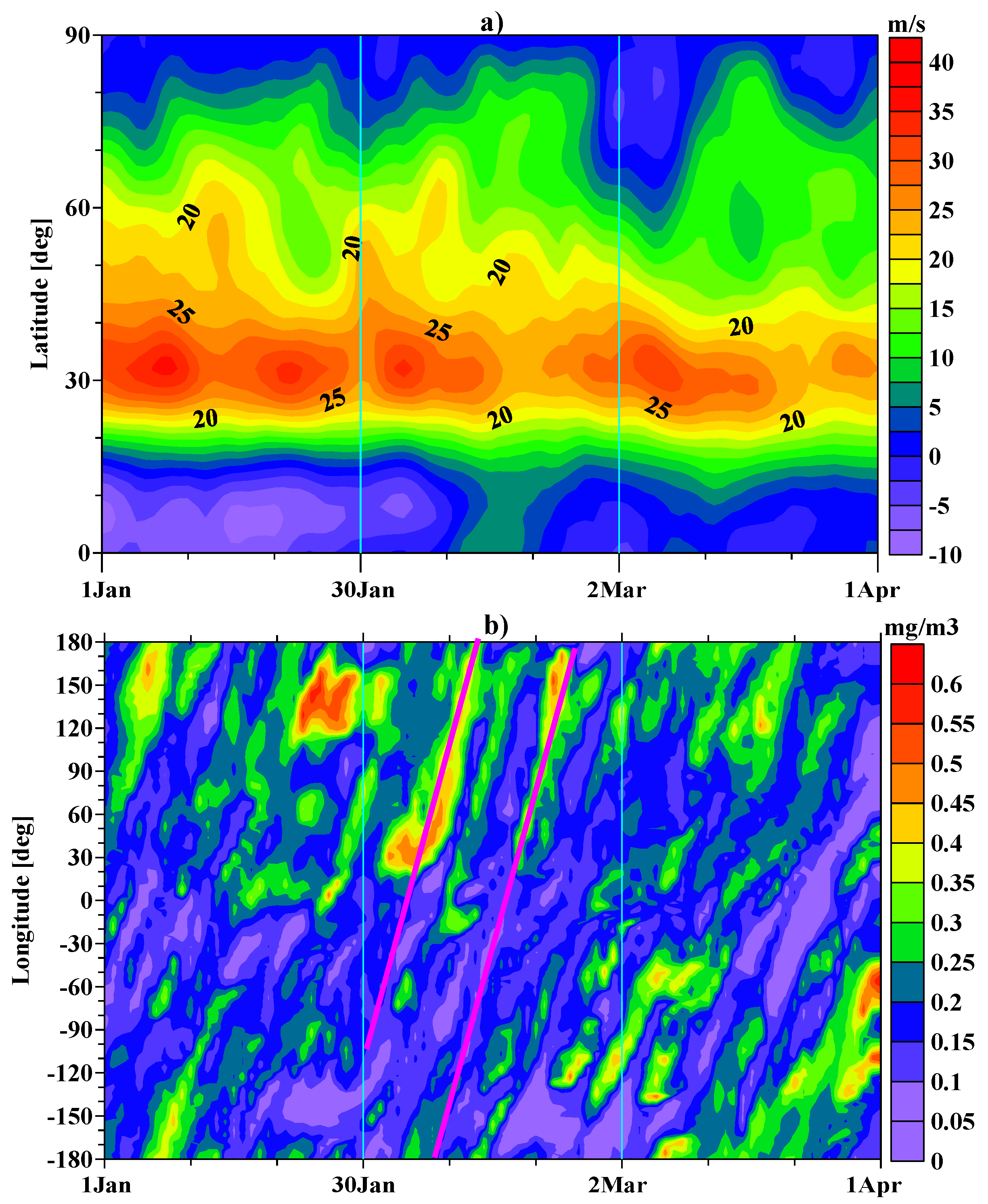
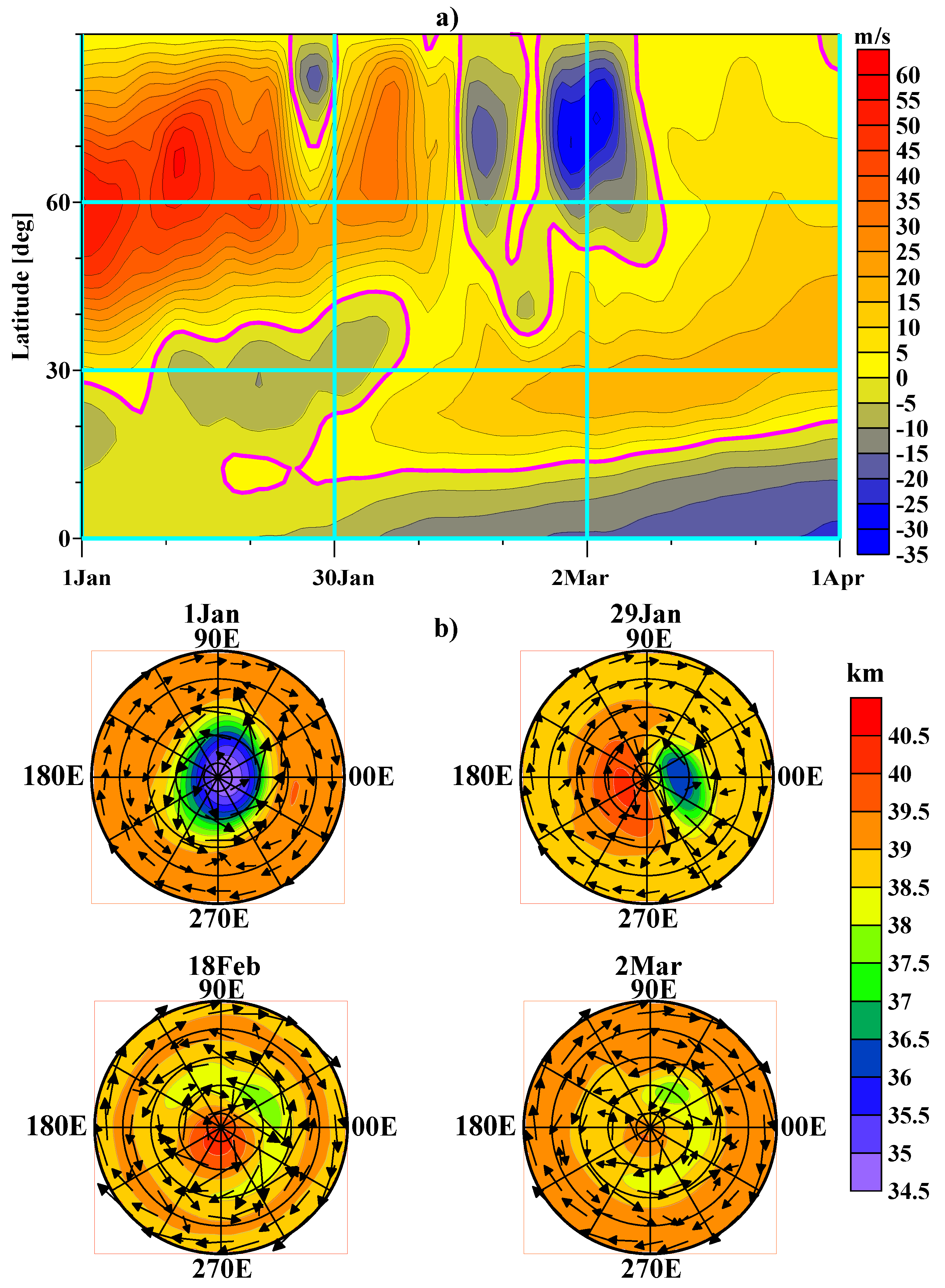
Figure 3a shows the evolution of the latitudinal distribution of the zonal mean of zonal wind for the Northern Hemisphere. The wind reversal in the minor stratospheric warming at the end of January reaches up to 70° N, and the major stratospheric warming in February occurs in two stages. Around the middle of February, the wind inversion reaches latitudes around 35° N. After a short-term recovery of positive direction at high latitudes in the end of February and at the beginning of March, a persistent area of negative wind direction reaching 50° N is formed. By the end of March, the wind direction again recovers and turns positive, which means that the stratospheric warming in February is not final.

The geopotential and horizontal wind direction maps in Figure 3b show the disruption of the circumpolar vortex during stratospheric warming. As indicated in the upper left panel of Figure 3b, relating to (1 January), the circumpolar region has low pressure, and the wind direction is from west to east. The behavior of the geopotential in the circumpolar region on 29 January shows the presence of two relatively symmetrically located areas. These regions are of low and high pressure, respectively, which determine two vortices, a cyclonic and an anticyclonic which lead to the penetration of warm air at the pole and a corresponding increase in the circumpolar temperature (which can be seen in Figure 2a). On 18 February, the two regions become asymmetric, with the region of increased pressure located near the pole, which may account for the adiabatic increase in polar temperature (see Figure 3b, bottom left panel). The increase in temperature at the pole at altitudes of about 40 km is accompanied by a decrease in temperature in the lower stratosphere, which can affect the ozone concentration. On 2 March, when maximum negative zonal winds values are observed, the two regions are again approximately symmetric (results shown in Figure 3b, bottom right panel).

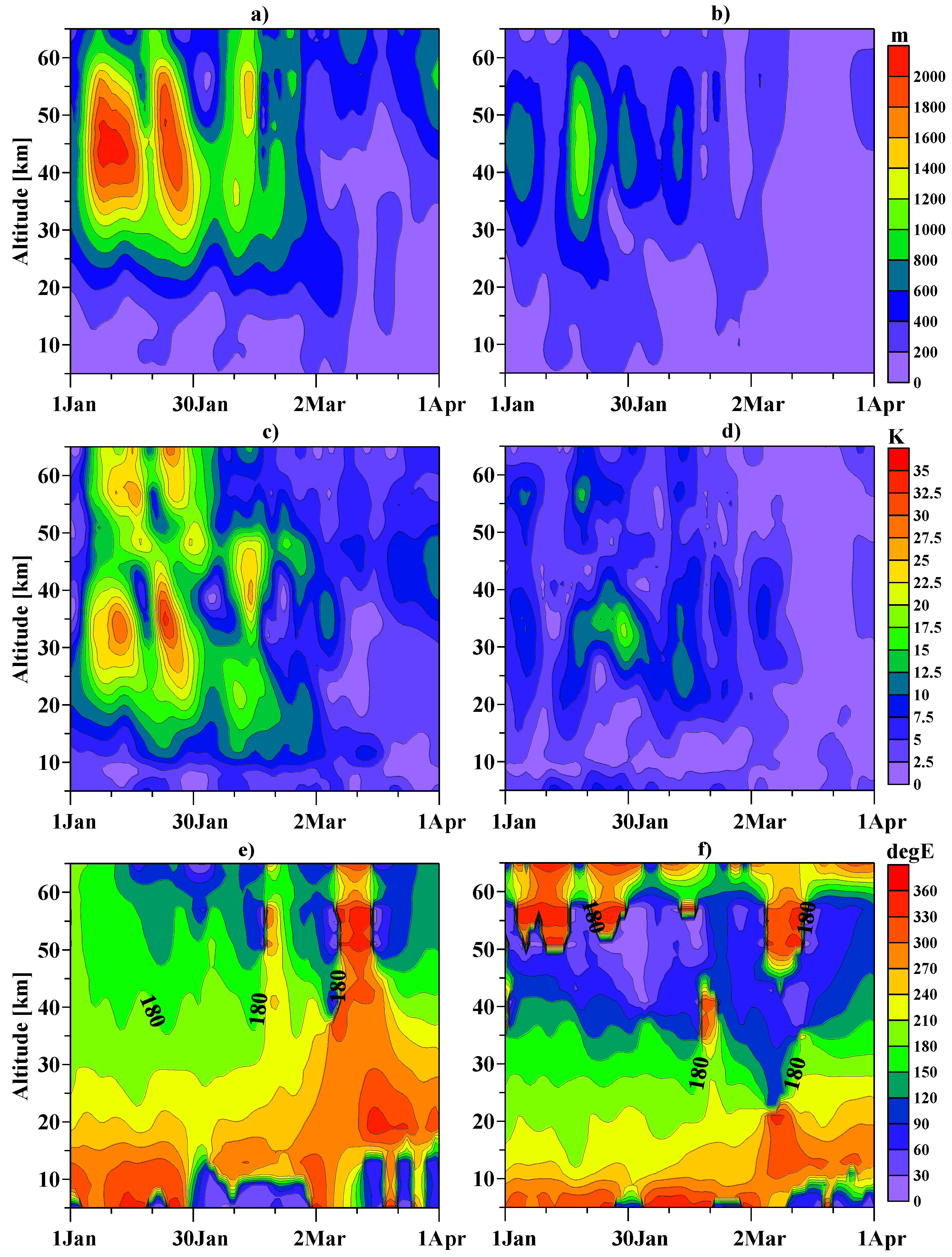
Figure 4 shows the vertical profiles of amplitudes and phases of wavenumber 1 (SPW1) and wavenumber 2 (SPW2) stationary waves in geopotential and temperature.

SPW1 is dominant in the months of January and February. The first activation of SPW1 in the beginning of January did not cause stratospheric warming, unlike the second (in the end of January) and the third (during March). The phase profiles of SPW1 show a steady propagation upwards from heights around and below the tropopause. Typical for the studied period are the relatively stable phases of SPW1 in January and February. At altitudes between 15 km and 25 km, where the main amount of stratospheric ozone is concentrated, they are close to 180° longitude. The amplitudes of SPW1 in temperature have significant values in this altitude interval and can be expected to influence the longitudinal distribution of stratospheric ozone concentration. The wave phases illustrated in Figure 4 represent the longitude at which the corresponding wave has a maximum.

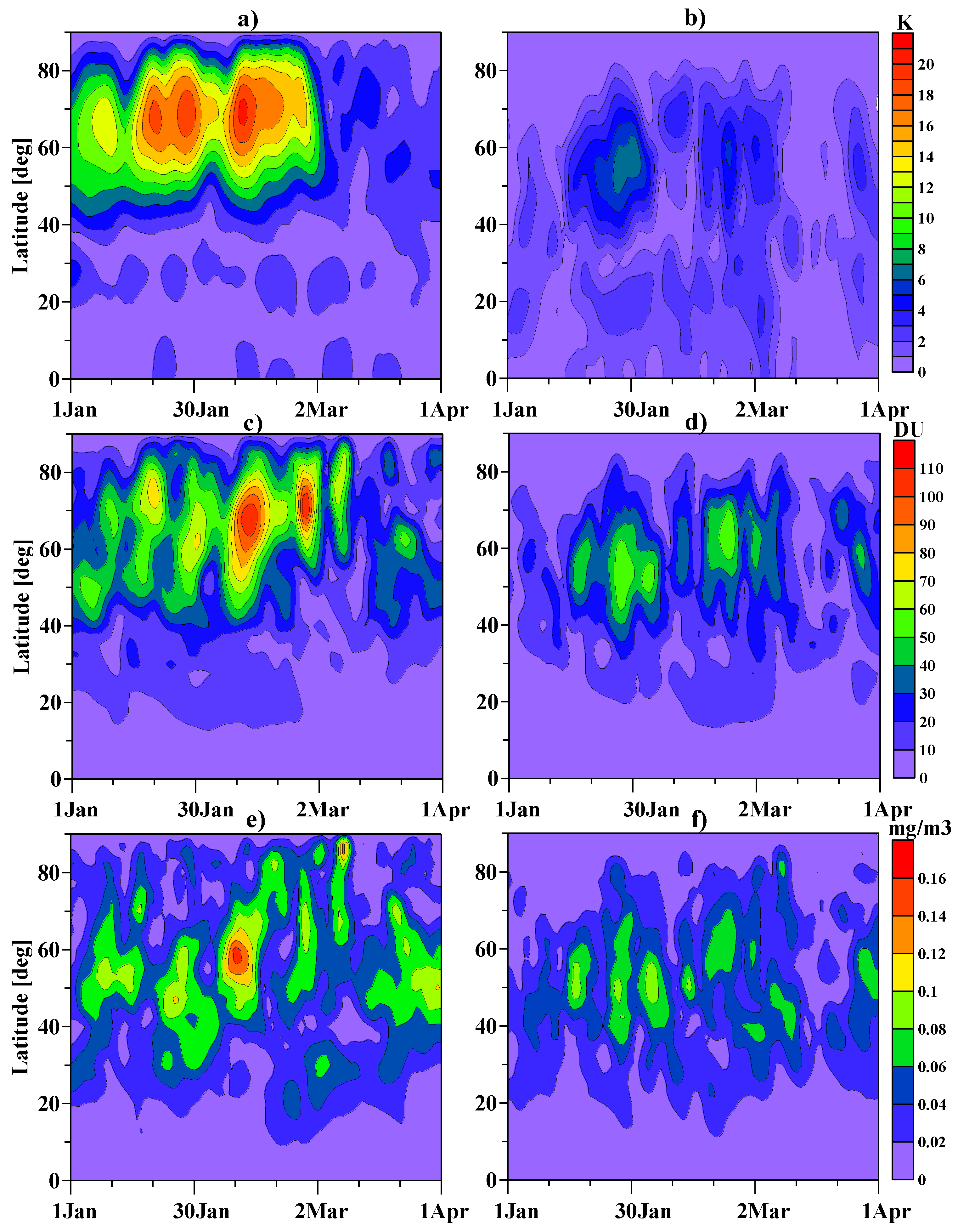
Figure 5 top row panels show the latitudinal distribution of amplitudes of the stationary waves (SPW1 and SPW2) in temperature at the 70 hPa level (about 19 km). The middle row of panels is an analogous representation but for TOC, and the bottom row of panels illustrates the same but for ozone concentration at the 70 hPa level. The selected level is close to the maximum of the ozone profile where the main mass of stratospheric ozone forming TOC is concentrated. Maximum amplitudes of SPW1 are observed in the middle of February. The figure shows that the maxima of SPW1 in temperature and TOC coincide in latitude (at about 70° N), while the maximum of SPW1 in ozone concentration is shifted to the south (at about 60° N). The amplitude dominant SPW1 characterizes the longitudinal inhomogeneity during the two stratospheric warmings in the end of January and in the middle of February. The close correspondence between temperature and ozone concentrations suggests a relationship between them.

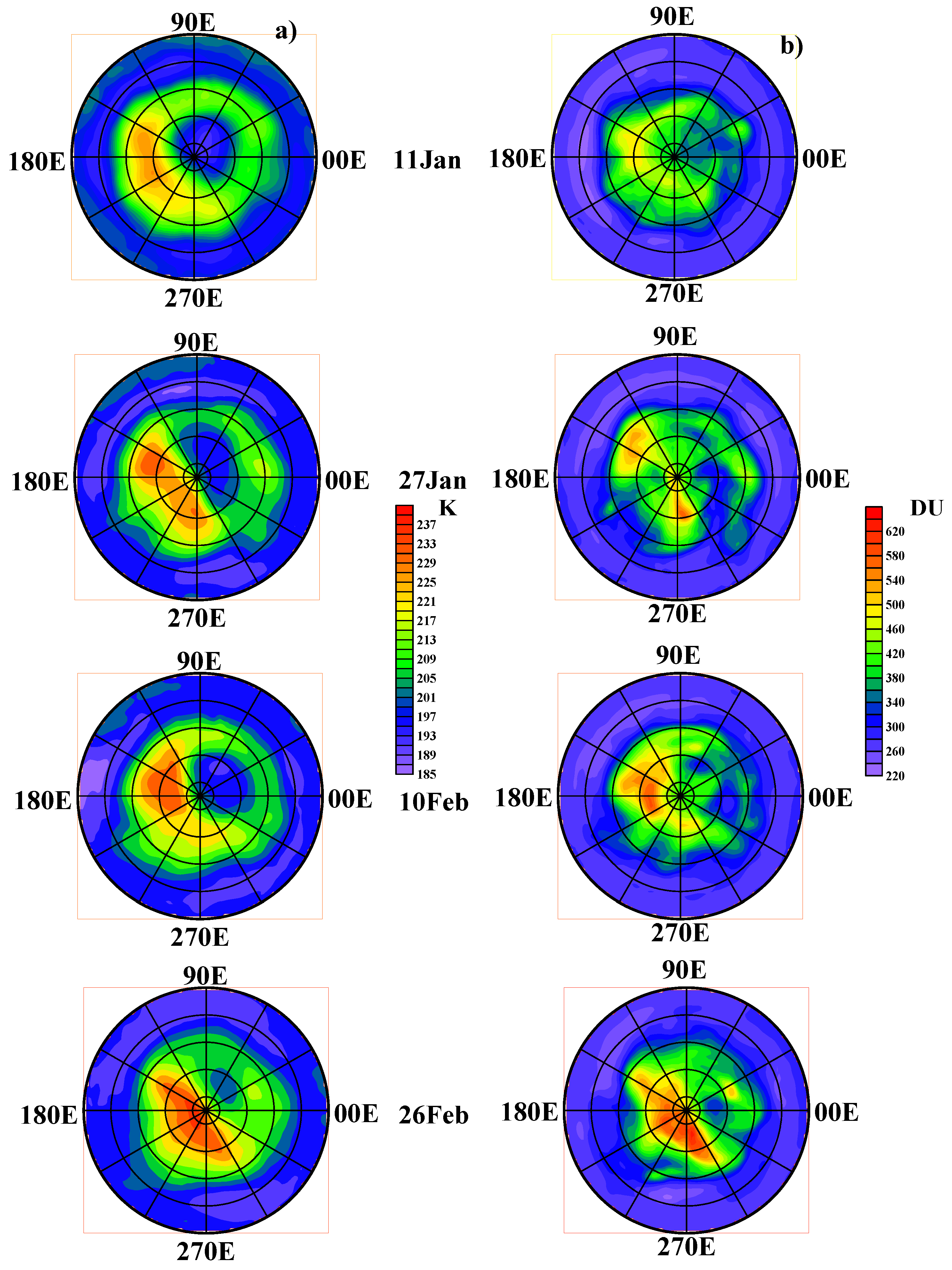
Figure 6 shows the latitudinal and longitudinal distribution of temperature at the 70 hPa level (left panels) and TOC (right panels) for days with high SPW1 values. The similarity in the distribution of the two considered quantities is obvious. The increased values of temperature and TOC are observed in the region north of 60° N with the maximum values occurring close to a longitude of 180° E, which confirms the SPW1 phase values shown in Figure 4. This similarity, which is observed in the four selected days provides additional reason to verify the existence of a correlation between the two quantities throughout the studied time interval.

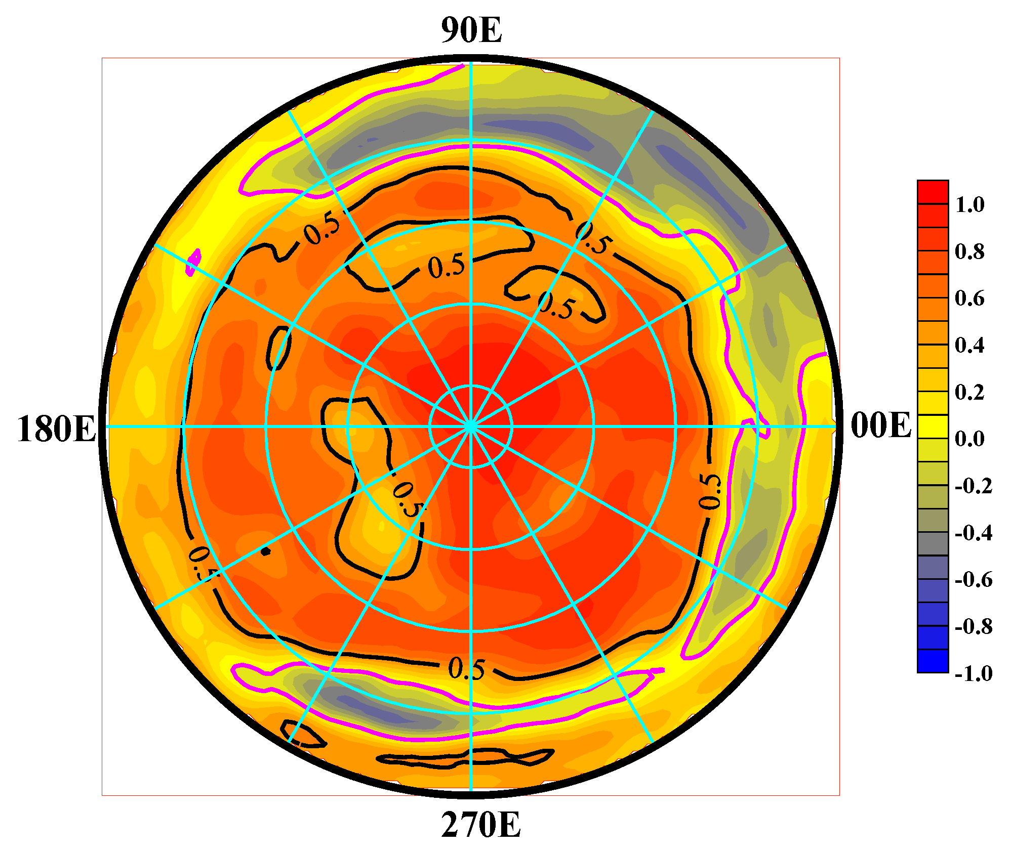
To solve the problem, the value of the normalized cross-correlation function (correlation coefficient) was calculated for each grid point based on the temperature and TOC data. The resulting correlation coefficient between the temperature at 70 hPa level and TOC is at zero time lag for the time period January–March 2023. The correlation coefficient values are shown in Figure 7. For latitudes north of about 25° N, the correlation is positive, with correlation coefficient values above 0.5 predominating. At lower latitudes, the correlation is weak, and in some areas it becomes negative. 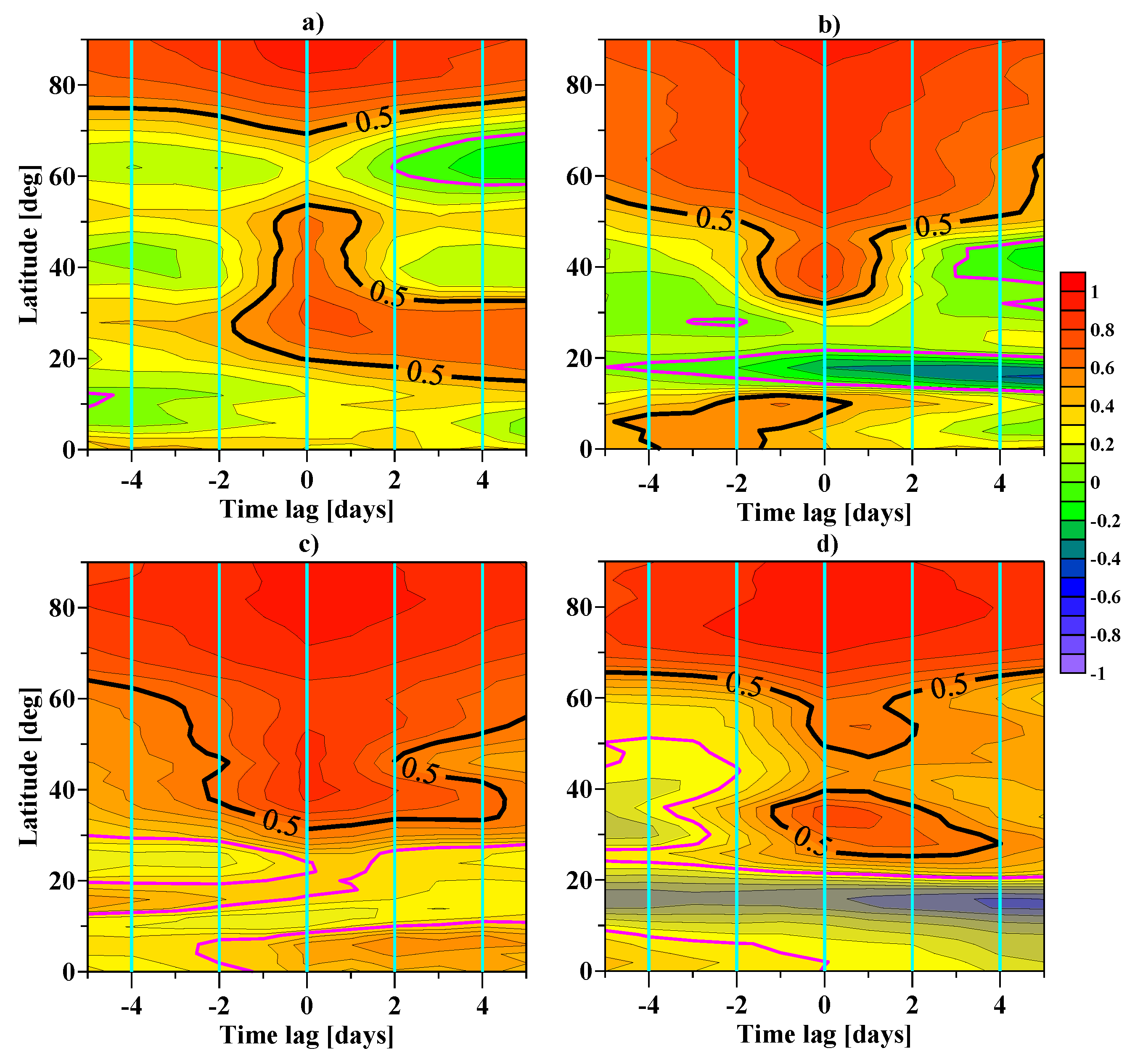The region of significant (greater than 0.5) correlation coincides with the regions shown in Figure 6, where for given days there is an apparent similarity in the latitudinal and longitudinal distributions of temperature and TOC. The cross correlations, which were calculated for each point and for the whole-time interval, show that the evolution of the two quantities is synchronous in time. The cross-correlation function was calculated for longitudes 180° W, 90° W, 0° E, and 90° E with time lags from −5 to 5 days. The results are shown in Figure 8.

For all shown longitudes at latitudes greater than 70° N, the cross-correlation is high and positive. It can be seen from the figure that at longitudes 180° W and 90° E at mid-latitudes, there is a region of reduced cross correlation, but also positive, which coincides with that shown in Figure 8. A significant time lag of TOC compared to temperature is observed at latitudes around 30° N and only at longitudes 180° W and 90° E. At these longitudes (180° W, 90° E), the maximum positive cross correlation is observed at lower altitudes than at 0° E and 90° W. The observed delay is probably related to differences in ozone lifetime at these altitudes. The presence of a time lag of TOC with respect to temperature is an argument for a causal relationship, and in this case variations in temperature cause variations in TOC.

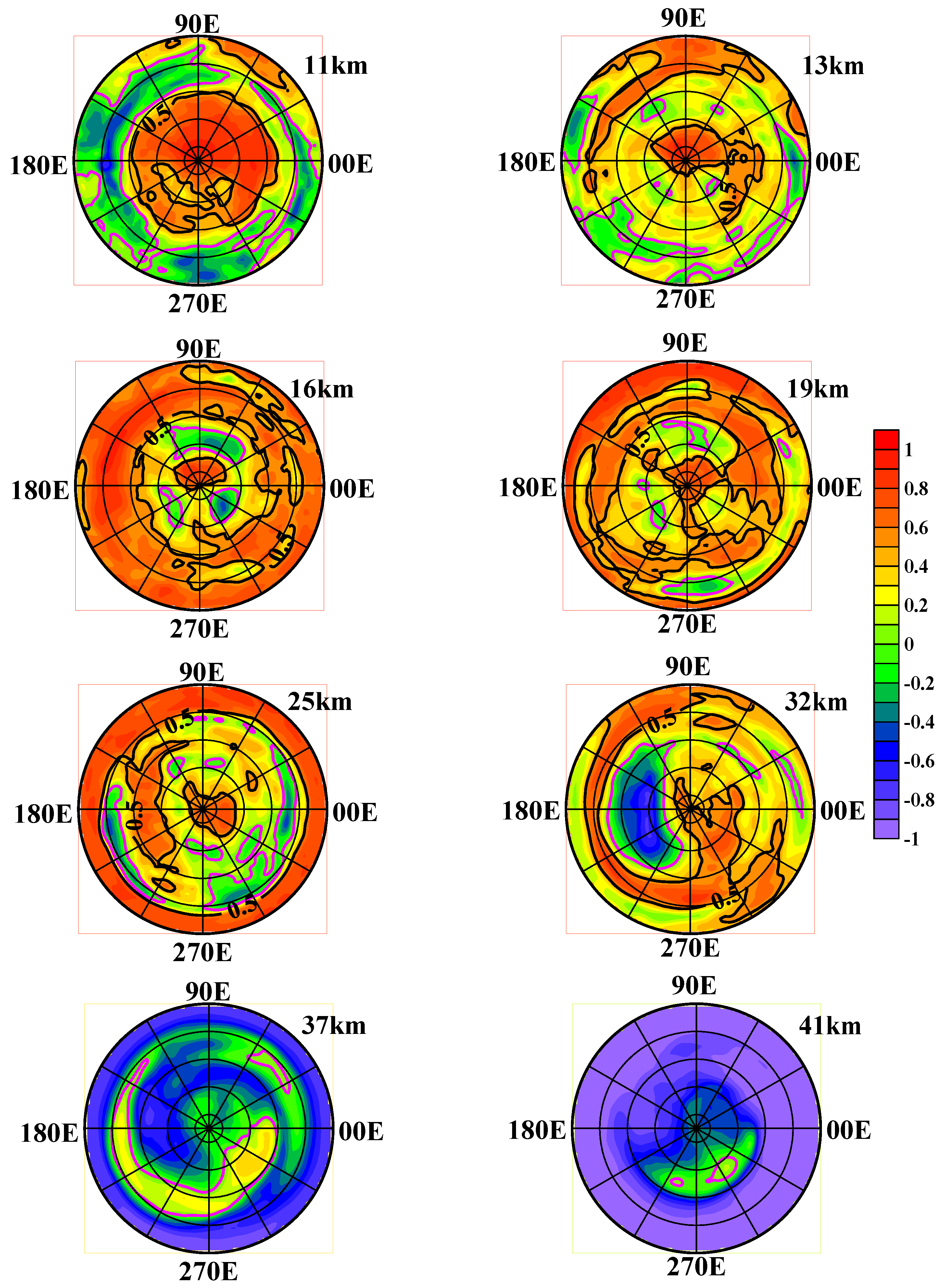
In order to clarify the nature of the influence of temperature on stratospheric ozone, the cross correlation between temperature and ozone concentration at different stratospheric altitudes was calculated. The results are shown in Figure 9. At altitudes of 11 km (200 hPa), the region of significant positive cross correlation is limited to latitudes higher than 40° N. Figure 9 shows that a positive correlation dominates at altitudes of 16 km and 19 km (100 hPa, 70 hPa) for the entire Northern Hemisphere. At an altitude of 25 km (30 hPa), a significant positive correlation exists at low latitudes lower than 20° N. At altitudes higher than 32 km (below 10 hPa), the correlation changes its sign and becomes negative. A possible explanation for the strong negative cross correlation at an altitude of about 32 km between 40° N and 60° N may be related to the evolution of the polar vortex (see Figure 3).

TOC as an integral of ozone concentration by altitude is predominantly determined by concentrations at levels below 32 km and changing the sign of the correlation above this level does not affect the behavior of TOC. The shift in the dependence of concentration on temperature sign should be explored through an examination of the altered physical mechanisms influencing this relationship. In the region around the maximum concentration in the stratosphere, ozone has a significant lifetime due to the strong reduction in the flux of UV radiation that destroys it. At these altitudes, transport processes are considered to predominate. At altitudes higher than 25 km, the absorption of UV radiation is strong, and it can be expected that the increase in temperature will support the dissociation of ozone, i.e., a decrease in ozone concentration. At an altitude of 41 km (3 hPa), which is close to the region of maximum absorption of UV radiation, the correlation is negative and high for almost the entire Northern Hemisphere.

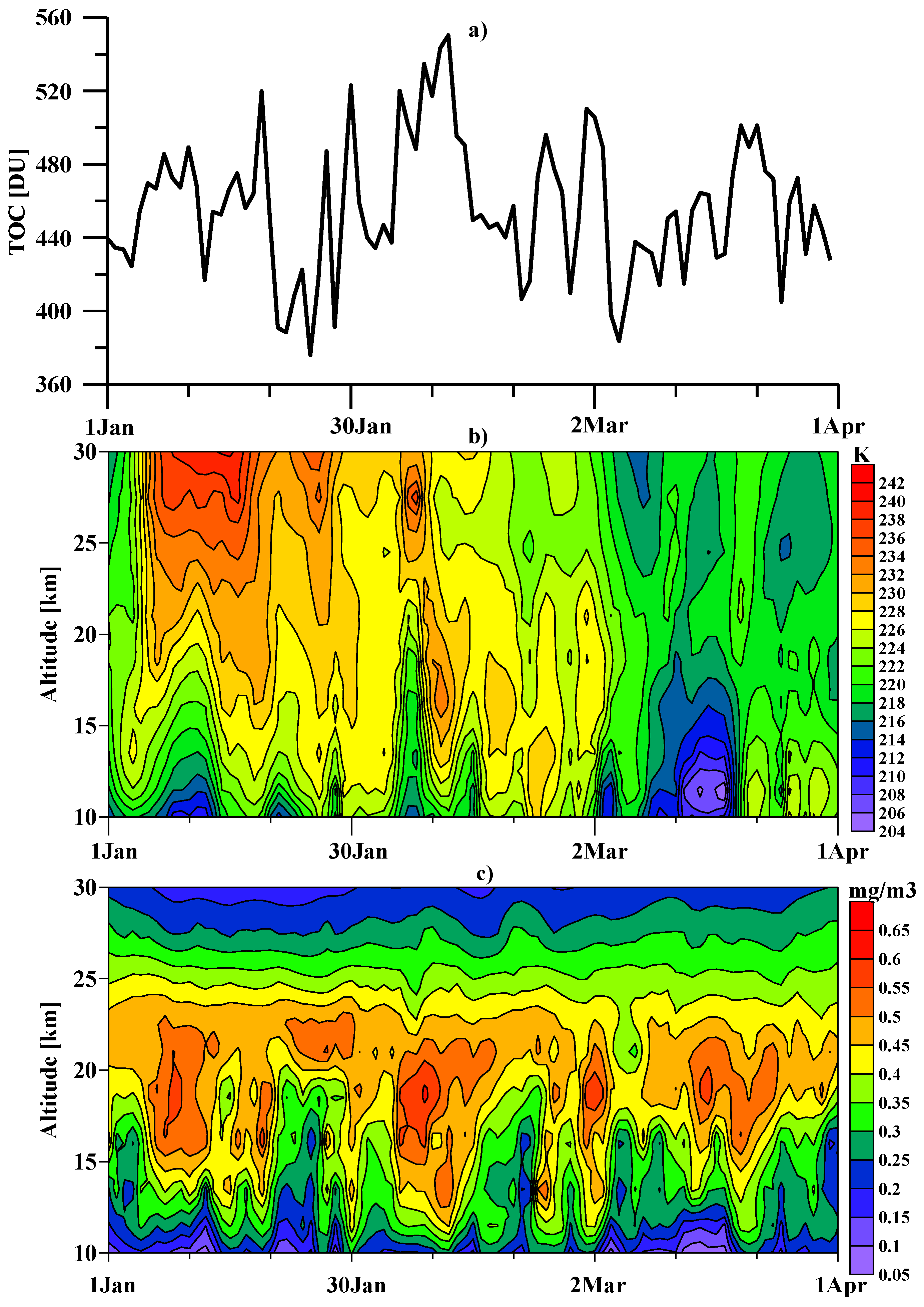
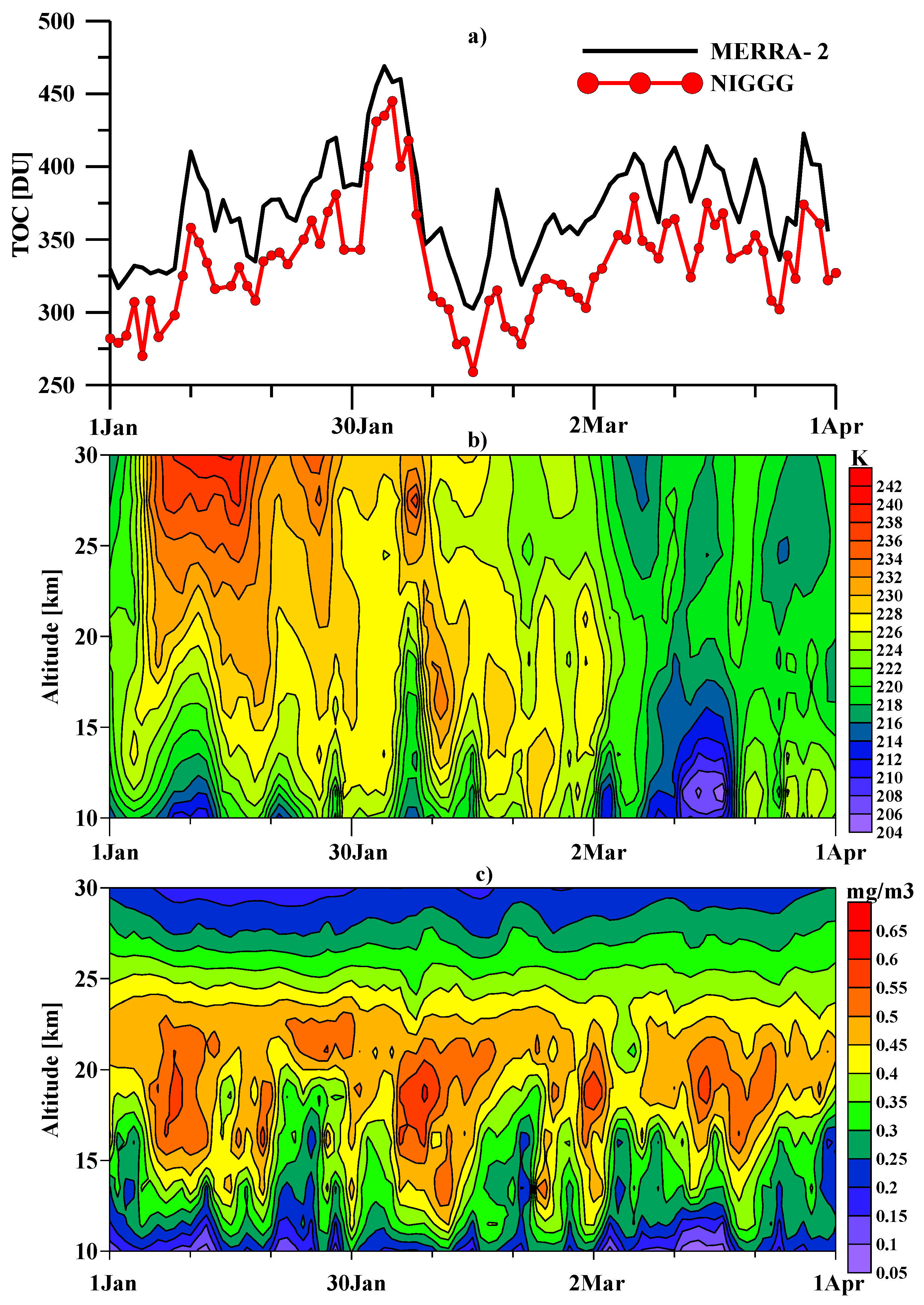
In order to evaluate the change in the ozone concentration profile, the course of the profile is considered for two selected points. One point has coordinates 42° N, 24° E and is presented in Figure 10. The chosen point is close to the coordinates of the city of the Sofia, where the TOC values shown in Figure 1 were measured and which are the starting point for the realization of the ideas contained in this study.

The TOC behavior calculated from MERRA-2 data shown in Figure 10a (upper panel) is consistent with those measured by the NIGGG-BAS instrumentation. Figure 10c (bottom panel) shows that the TOC maximum during the first 10 days of February is caused by the increase in ozone concentration at levels below 21 km. The increase in ozone concentration is particularly noticeable at altitudes between 10 km and 15 km. In this case, the maximum of the ozone layer is shifted at a lower altitude. At these altitudes, there is also an increase in temperature, but it is not significant. The subsequent strong decrease in TOC around the middle of February is apparently related to the sharp decrease in temperature at all altitudes from 10 km to 30 km, which decreases ozone concentrations at all altitudes. At the end of February, both the TOC and the altitude of the concentration maximum were normalized. It is observed that the short-term increases in temperature at the 11 km level are synchronous with the increases in ozone concentration at the same levels, illustrating the positive correlation between temperature and ozone concentration at 11 km, shown in Figure 9.

The other selected point has coordinates 60° N, 180° W and is shown in Figure 11. It was chosen due to the fact that maximum temperature and TOC values were observed there (see Figure 6).

For comparison with the results in Figure 10, Figure 11 shows the same quantities but for 60° N, 180° E. The analysis shows that the increase in TOC around 10 February is also related to the increase in temperature and ozone concentration at altitudes between 11 km and 15 km.

Some insight into the horizontal transport of the ozone concentration anomalies is provided by Figure 12b (bottom panel), which shows the longitudinal distribution of the ozone concentration at the 100 hPa level (~16 km) at latitude 42° N. The figure clearly shows the increase in ozone concentration on 5 February, also shown in Figure 10. This anomaly migrated eastward at about 270° for 14 days. It is noticed that throughout the three-month period, there is an eastward drift of the anomalies at this altitude with a similar speed, which corresponds to a speed of 19.6 m/s.

Figure 12a (top panel) shows the variability of the zonal mean of zonal wind at the same altitude level. At latitudes around 40° N, the zonal wind speed is positive (west–east) throughout the considered period and varies around 20–25 m/s, which is close to the drift speed of ozone concentration inhomogeneities.

4. Discussion and Conclusions

The considered winter period January–March 2023 is characterized by activity of stationary Planetary Waves with wave number 1 (SPW1) in the stratosphere at high mid-latitudes in the Northern Hemisphere. Three SPW1 activations were observed in the geopotential field—two in January and one in March. The second causes minor stratospheric warming, and the third major. The maximum amplitudes of stationary waves in the geopotential reach altitudes of about 45 km. The corresponding maximum amplitudes of SPW1 in the temperature field are located below and above this altitude due to the dependence of the temperature on the geopotential gradient. As a result, longitudinal inhomogeneities in temperature are significant at altitudes around 20 km, where maximum of the stratospheric ozone concentration is. This fact makes it possible to investigate the variations of TOC under the influence of temperature anomalies.

As a result of this investigation, it is established that the latitudinal and longitudinal distributions of TOC have a remarkable similarity with that of the temperature at altitudes near the altitude of the ozone concentration maximum. It is found that for latitudes north of 20° N, there is a high (above 0.5) correlation between temperature and TOC over time [34]. The correlation between the temperature at individual stratospheric levels and ozone concentration was also investigated. It turns out that in the region around the ozone concentration maximum, the correlation is high and positive, which is very similar to the correlation with TOC. An interesting result of this study is the correlation of altitude near the tropopause, which is high and positive at latitudes higher than 40° N and negative at lower latitudes. With an increase in altitude to a level of about 37 km, the sign of the correlation changes to negative, which is obviously related to the decrease in the lifetime of stratospheric ozone and the corresponding predominance of ozone dissociation mechanisms dependent on temperature. However, at these altitudes, the ozone concentration is small and does not significantly affect TOC. A detailed study of the variations in the ozone concentration profile at two selected points in the Northern Hemisphere shows that the anomalous increases in TOC during stratospheric warming are due to an increase in the ozone concentration in the altitude range between 10 km and 15 km, i.e., below the ozone layer maximum. These increases in some cases lead to a decrease in the altitude of the maximum.