Design and Verification of Assessment Tool of Shortwave Communication Interference Impact Area

Abstract

In the field of electronic communication warfare, accurately predicting the range and intensity of shortwave interference signals presents a significant challenge due to the complex interplay between the ionospheric parameters and the electromagnetic environment. To address this challenge, we designed a novel tool to assess the interference impact area of shortwave interference signals in a dynamically changing ionospheric environment. Considering sophisticated ionospheric radio wave propagation models and innovative spatial grid methods, this tool finishes the comprehensive spatial distribution of the interference impact area and delivers grid-based insights into the interference intensity. Furthermore, the test verification of the tool demonstrated a mean error of 8.42 dB between the measured and simulated results, underscoring the efficacy and reliability of this tool. This pioneering work is poised to make substantial contributions to the field of communication electronic warfare and holds significant promise for guiding the development of interference countermeasures.

1. Introduction

Shortwave communication is an essential wireless communication method that has extensive applications in fields such as national defense, aviation, maritime, weather forecasting, broadcasting, and agriculture [1]. However, with the continuous advancement of communication technology, shortwave communication systems are increasingly confronted with more interference issues [2]. Shortwave communication interference refers to the occurrence of interference signals during the process of shortwave communication due to various reasons, thereby reducing the performance and reliability of the communication system [3]. Interference signals can originate from other communication systems, power line disturbances, atmospheric electrical storms, etc. Interference not only degrades the communication quality, causing noise and distortion but can also lead to interruptions and failures in communication systems, posing significant challenges for the communication service providers and users. Evaluating the interference impact area of shortwave communication can guide the planning and construction of communication systems, optimize antenna placement and height, select suitable operating frequencies, and enhance the reliability and stability of communication. Simultaneously, assessing the interference impact area in communication can support the research and application of electronic warfare technologies.

Numerous research endeavors have assessed and alleviated interference in shortwave communication systems. These papers encompass diverse subjects, spanning interference evaluation methodologies, models for interference in tropical regions, propagation analysis utilizing artificial neural networks, the impacts of ionospheric scintillation, techniques for interference mitigation, and methods employing optimization algorithms [4,5,6,7]. Additionally, the researchers delve into inquiries regarding the influence of interference on software-defined radios, creating a compact channel sounder for shortwave radio communications and predicting electronic equipment performance under specific radiation conditions [8,9,10,11]. The central emphasis of these studies lies in methodology, underscoring the critical importance of developing a robust tool for precise interference assessment in shortwave communication systems. These approaches aim to effectively address interference issues, optimize the system design, and formulate appropriate countermeasures. By synthesizing findings from many studies, many reviews provide valuable insights into the current state of research in this pivotal area [12,13,14].

To address the challenge of accurately predicting the range and intensity of shortwave interference signals in the complex interplay of ionospheric parameters and the electromagnetic environment, this paper introduces a groundbreaking assessment tool designed to evaluate the interference impact area in shortwave communication. By leveraging ionospheric radio wave propagation effect models and spatial grid processing methods, the tool offers a unique capability for longitudinal and latitudinal spatial assessment of the interference footprint. By integrating the spectral characteristic parameters of shortwave interference devices with ionospheric data, it delivers a detailed spatial distribution of the interference impact area and grid-based information on interference intensity. The extensive research and rigorous validation of this tool has significantly advanced our understanding of the propagation characteristics of shortwave interference signals, enabling a more effective assessment of the range and intensity of the interference footprints. This pioneering work not only showcases the authors’ substantial contribution to the field but also provides an indispensable reference for the high-level development of communication electronic warfare and interference countermeasures.

2. Design and Method

This section introduces the assessment tool used to determine the impact areas of the shortwave communication interference. This tool considers various inputs, including parameters related to shortwave interference devices, databases containing ionospheric environmental data, and specific methods for assessing the impact of areas of interference. The primary objective of this assessment was to delineate the range of the interference footprint on the ground, representing the areas where the interference signals emitted from the antennas and reaching the surface through ionospheric reflection had an impact.

The evaluation technique for shortwave sky–wave interference impact areas was designed to assess the effectiveness of interference devices by meticulously evaluating the strength of the electromagnetic interference signals. These signals are effectively radiated from the antenna aperture, considering the transmission losses incurred through the ionosphere to reach the specific impact points on the ground.

This tool was designed with a hierarchical structure comprising the base, data, model, analysis, and application layers, as illustrated in Figure 1.

(1)

Base layer

This layer encompasses the operating system, office automation system, two-dimensional military geographic information system, three-dimensional rendering engine, and device drivers, serving as the foundation for all applications.

(2)

Data layer

This layer comprises an equipment frequency information database, radio wave environment database, electromagnetic environment sample database, spectrum characteristics database, and geographic information database, providing the necessary support data for system applications.

(3)

Model layer

The Model Layer is divided into the analysis, computation, display model and the electromagnetic radiation characteristic parameter model. The analysis, computation, and display models include radio wave propagation, electromagnetic interference analysis, radio wave environments, and station display models. They provide bottom-level calls for the Analysis Service Layer, ensuring the accuracy of upper-level analysis and computation.

(4)

Service layer

The Analysis Service Layer mainly includes geographic information services, radio wave propagation calculation services, electromagnetic interference analysis services, electronic equipment information collection services, essential data processing services, display data processing services, and frequency efficiency analysis services, providing analysis services for the application layer.

(5)

Application layer

The Application Layer directly caters to users, offering business functions such as interference impact area analysis, communication frequency analysis, multisystem cooperative interference efficiency analysis, interference position analysis, and shortwave deployment analysis. The tool supports customization and can be flexibly deployed at designated operator workstations. It provides users with a GUI graphical interface and callable API application interfaces.

Based on the design above structure, we developed a tool for assessing the impact of interference in shortwave communication using the C++ programming language. In the initial stages, we crafted models for the antenna patterns of log-periodic antennas at 5, 7, and 9 MHz, based on the physical parameters of the shortwave devices. Subsequently, we established a database documenting the ionospheric conditions across the evaluation area. We constructed a grid matrix to evaluate the interference coverage area’s field strength. This matrix facilitates the computation of the field strength at all points within the grid, offering a comprehensive assessment. Finally, a shortwave communication interference impact area evaluation tool is employed to assess and visually present the results.

2.1. Equipment Parament

To accurately evaluate the field strength at a target point, it is crucial to model the antenna pattern according to the physical characteristics of the equipment. The shortwave communication interference device employs a logarithmic periodic antenna to generate a shortwave communication interference environment spanning the 2 to 30 MHz frequency range. The critical operational parameters are presented in the

Table 1. Equipment operating parameter data.

Item	Parameter
Size	22 antenna arrays, the longest array is 32.05 m, the shortest array is 1.76 m, and the erection area is 32 m × 57 m
Antenna type	Log-periodic antenna
Antenna gain	6–8 dB
Impedance	50 Ω
Power	15 kW
VSWR	≤2
Main beam elevation angle	40°–60°
Interference frequency step	1 MHz

.

Based on the physical structure of the equipment’s antenna, a modeling of its antenna pattern has been conducted, and the directional pattern is shown in Figure 2, Figure 3 and Figure 4.

To facilitate sky–wave propagation of shortwave interference equipment, adjustments to the antenna’s horizontal azimuth and pitch angles are imperative. This necessitates rotating the three–dimensional antenna body data to accommodate azimuth and pitch modifications. Considering the original coordinate system as (x′, y′, z′), it must be transformed into the coordinate system (x, y, z) with rotation angles denoted as follows: θ is the rotation angle of the zx axis in the Y series, φ is the rotation angle of the yz axis in the X series, and ψ is the rotation angle of the xy axis in the Z series.

The rotation matrix R is expressed as follows:

$$x\left(\phi \right)=\left(\begin{array}{ccc}\cos \phi & \sin \phi & 0\\ -\sin \phi & \cos \phi & 0\\ 0& 0& 1\end{array}\right),$$

(1)

$$y\left(\theta \right)=\left(\begin{array}{ccc}1& 0& 0\\ 0& \cos \theta & \sin \theta \\ 0& -\sin \theta & \cos \theta \end{array}\right),$$

(2)

$$z\left(\psi \right)=\left(\begin{array}{ccc}\cos \psi & \sin \psi & 0\\ -\sin \psi & \cos \psi & 0\\ 0& 0& 1\end{array}\right),$$

(3)

$$R\left(\psi ,\theta ,\phi \right)=\left(\begin{array}{ccc}\cos \psi \cos \phi -\sin \psi \sin \phi \cos \theta & \sin \psi \cos \theta +\cos \psi \sin \phi \cos \theta & \sin \phi \cos \theta \\ -\cos \psi \cos \phi -\sin \psi \sin \phi \cos \theta & -\sin \psi \sin \phi +\cos \psi \cos \theta & \cos \phi \sin \theta \\ \sin \psi \sin \theta & -\cos \psi \sin \theta & \cos \theta \end{array}\right),$$

(4)

Based on the geometric principles of rotation and the rules of matrix multiplication, geometric transformations are applied to the shapes of three-dimensional antenna directional patterns using a Cartesian coordinate system, resulting in a rotated three-dimensional antenna directional pattern [15,16].

2.2. Ionospheric Environmental Database

The propagation and reception of shortwave interference signals are influenced by ionospheric parameters and the electromagnetic environment, significantly impacting the quality and reliability of shortwave communication. Ionospheric parameters, such as density, altitude, and critical frequency, can influence the propagation path and attenuation of shortwave signals. Variations in these parameters can lead to phenomena like reflection, refraction, and scattering of shortwave signals, resulting in changes in the propagation paths, potential attenuation, and multipath interference.

In addition to ionospheric parameters, the electromagnetic environment, which includes other electromagnetic wave sources and signals such as lightning activity, electromagnetic radiation, and artificial interference, can also adversely affect the reception of shortwave interference signals.

An accurate understanding of the ionospheric parameters and the surrounding electromagnetic environment is crucial for conducting assessments of shortwave communication interference impact areas. Therefore, it is necessary to establish an ionospheric environmental database for the assessment of the region’s airspace using data from domestic radio wave environmental observation stations. The specific data contents are detailed in the

Table 2. Ionospheric parameter data table.

Parameter	Units	Description
foE	MHz	The critical frequency of the ionospheric E layer
foF2	MHz	The critical frequency of the ionospheric F2 layer
M(3000)F2	-	Propagation factor of 3000 km
Sunspot	-	Solar activity parameter
Ionospheric density	el/m3	The electron density distribution in the ionosphere
Ionospheric height	m	The bottom or top altitude of the ionosphere
Ionospheric temperature	K	The temperature distribution of gases in the ionosphere
Electron density profiles	el/m3	The variation of electron density with altitude in the ionosphere

.

2.3. Shortwave Communication Interference Zone Assessment Method

2.3.1. Shortwave Interference Zone Field Strength Assessment

The antenna gain at a specific angle (α for azimuth and β for elevation) was determined by extracting the corresponding value from the antenna pattern data. Subsequently, the interference strength at the reception point of the grid link for N modes (where N is chosen to include both the F2 and E modes) can be obtained, as detailed in [17,18].

$$E_s = 10 {\log }_{10} {\displaystyle \sum _{w = 1}^N{10}^{E_w/10}}$$

(5)

For each mode w, the field strength is given by:

E_w = 136.6 + P_t + G_t + 20 log f − L_b

(6)

where f is the transmitting frequency (MHz), P_t is the transmitter power (dBkW), G_t is the transmitting antenna gain at the required azimuth angle and elevation angle relative to an isotropic antenna (dB), and L_b is the ray path basic transmission loss for the mode under consideration, given by

L_b = 32.45 + 20 log f + 20 log p′ + L_i + L_m + L_g + L_h + L_z

(7)

where L_g is the summed ground-reflection loss at intermediate reflection points and L_g = 2(n − 1), L_h is the factor to allow for auroral and other signal losses, L_z is a term containing those effects in sky-wave propagation not otherwise included in this method, and the present recommended value is 8.72 dB, p′ is the virtual slant range (km) as

$$p\prime =2R_e{\displaystyle \sum _1^n\left[\frac{\sin \left(d_n/2R_e\right)}{\cos \left(\Delta +d_n/2R_e\right)}\right]}, R_e\mathrm{is} \mathrm{earth} \mathrm{radius}, \mathrm{and} d \mathrm{is} \mathrm{distance}$$

(8)

L_i is the absorption loss (dB) as

$$L_m=\{\begin{array}{ll}0\hfill & ,f\le \mathrm{MUF}\left(n,t\right)\hfill \\ \min \left\{130{\left[f/\mathrm{EMUF}-1\right]}^2,81\right\}\hfill & ,\mathrm{E}-\mathrm{layer}\mathrm{model}\mathrm{and} f>\mathrm{EMUF}\hfill \\ \min \left\{36{\left[f/\mathrm{F}2\mathrm{MUF}-1\right]}^{\frac{1}{2}},62\right\}\hfill & ,\mathrm{F}2-\mathrm{layer}\mathrm{model},f>\mathrm{F}2\mathrm{MUF}\hfill \end{array}$$

(9)

L_m is “above-the-MUF” loss as

$$L_i=\frac{n\left(1+0.0067R_{12}\right)\sec i_{110}}{{\left(f+f_L\right)}^2}\cdot \frac{1}{k}{\displaystyle \sum _{j=1}^{k}A{T}_{noon}\frac{F\left({\chi }_j\right)}{F\left({\chi }_{jnoon}\right)}}{\phi }_n\left(\frac{f_V}{\mathrm{foE}}\right)$$

(10)

where R₁₂ is the 12-month smooth mean value of the sunspot, i₁₁₀ is the angle of incidence at 110 km, f_L is the electron gyrofrequency, AT_noon is the absorption factor at local noon for the penetration point, and R₁₂ = 0 given as a function of geographic latitude and month, χ is solar zenith angle at the penetration point or 102° whichever is the smaller, χ_jnoon is value of at local noon, F(χ) is cos^p(0.881χ) or 0.02 whichever is greater, φ(f_V/foE) is absorption layer penetration factor at the penetration point given as a function of the ratio of equivalent vertical-incidence wave frequency f_V.

2.3.2. Interference Zone Grid Matrix

Given the grid link OS, where the transmitting point is O (x′, y′), and the receiving point is S (x, y) = S (X₀ + 1/60 × S₁, Y₀ + 1/60 × S₂). By calculating the interference intensity at reception point M along the OS link as a function of the parameter x related to feature C, we establish the grid link matrix R according to the rule of selecting grid points from left to right and from bottom to top. The grid division from left to right involved partitioning the maximum longitudinal range of the interference zone into 60 segments per degree. Therefore, the longitude of the grid points was given by x_i = x₀ + i × (1/60). The bottom-to-top grid division method involved partitioning the maximum latitude range of the interference zone into 60 segments per degree. Therefore, the latitude of the grid points is given by y_i = y₀ + j × (1/60). The grid point matrix S is expressed as follows:

$$S=\left[\begin{array}{cccc}\left(x_0,y_j\right)& \left(x_0,y_j\right)& \cdots & \left(x_0,y_j\right)\\ ⋮& ⋮& \cdots & ⋮\\ \left(x_0,y_1\right)& \left(x_1,y_1\right)& \cdots & \left(x_i,y_1\right)\\ \left(x_0,y_0\right)& \left(x_1,y_0\right)& \cdots & \left(x_i,y_0\right)\end{array}\right],$$

(11)

In the equation, x_i is the longitude coordinate of the grid point, y_j is the latitude coordinate of the grid point, and (x_i, y_j) represents the position coordinate on the geographic coordinate system, that is, the grid coordinate corresponding to the i-th column of the longitude grid and the j-th row of the latitude grid.

Then the grid link R_ij = (O, S_ij), which

$$R=\left[\begin{array}{ccc}{R}_{0j}& \cdots & R_{ij}\\ ⋮& \ddots & ⋮\\ R_{00}& \cdots & R_{i0}\end{array}\right],$$

(12)

The interference intensity characteristic value l is corresponding to the grid link, and the interference intensity grid matrix is denoted as L = (R, l) = (O, S, l), which

$$L=\left[\begin{array}{cccc}{l}_{0j}& l_{1j}& ⋮& l_{ij}\\ ⋮& ⋮& \cdots & ⋮\\ l_{01}& l_{11}& \cdots & l_{i1}\\ l_{00}& l_{10}& \cdots & l_{i0}\end{array}\right]$$

(13)

where l_ij represents the characteristic value of the interference intensity corresponding to the link between the grid S coordinates of the i-th column of the longitude grid, the j-th row of the latitude grid, and the transmitting point O of the jamming device.

3. Simulation and Results

To assess the interference coverage area of shortwave communication, we developed a tool that utilizes an ionospheric radio wave propagation model and spatial grid-based methods to evaluate shortwave signals. Based on the equipment mentioned above, parameter modeling, ionospheric parameter model, radio wave propagation model, and interference area assessment, the field strength in the coverage areas of the 3 link sets was evaluated according to the test link configurations and interference device deployments, specifically:

(1)

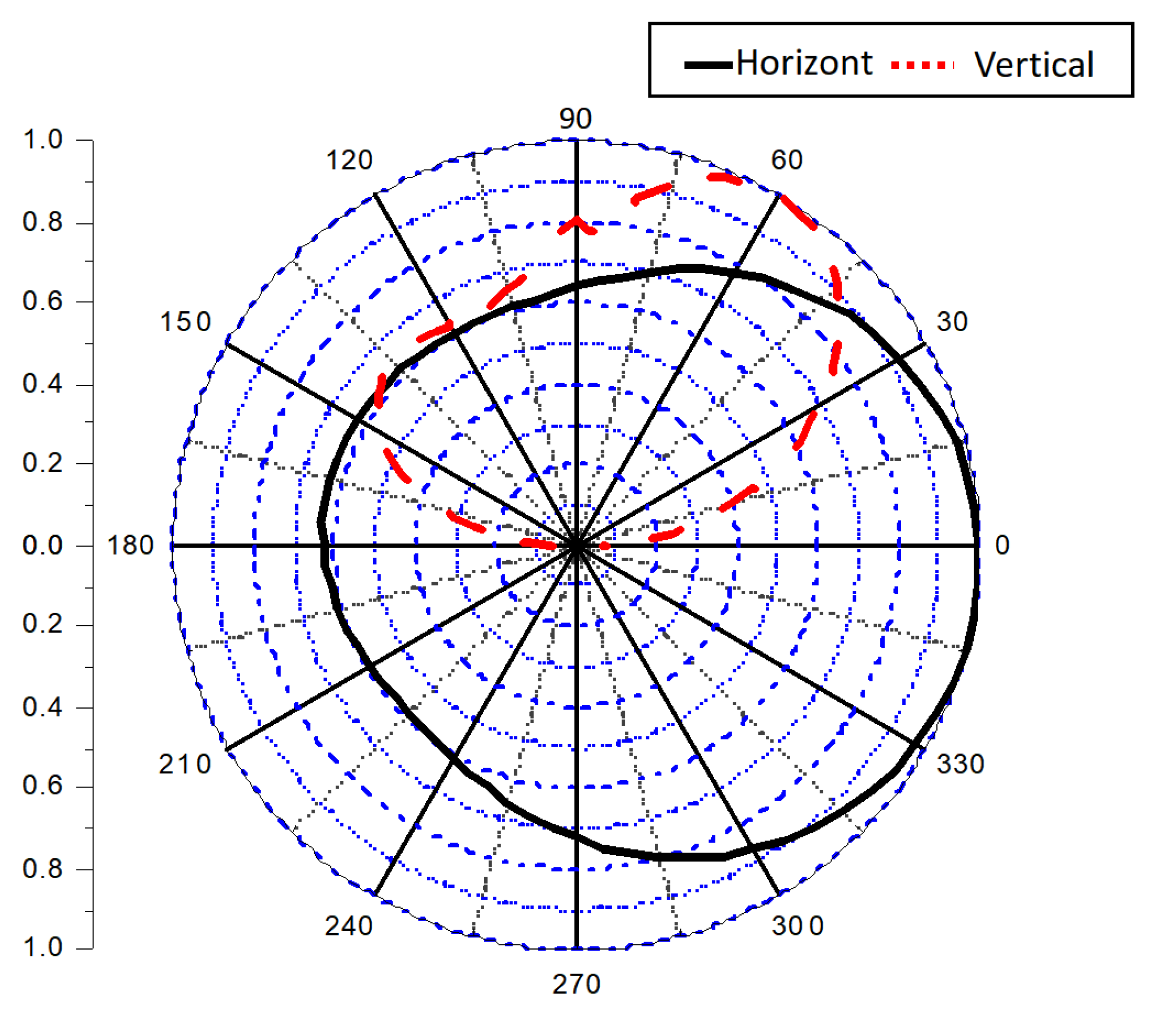
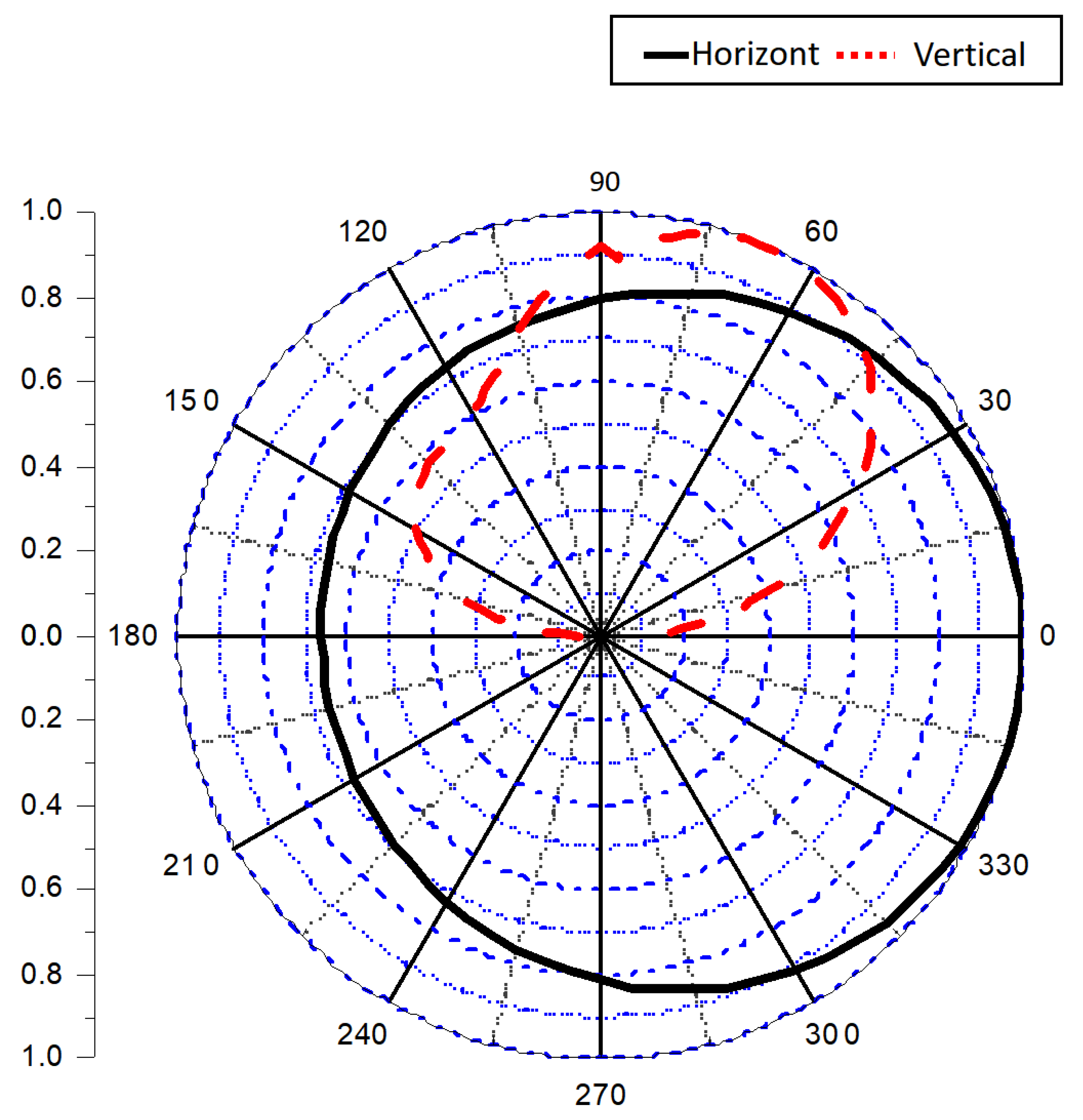
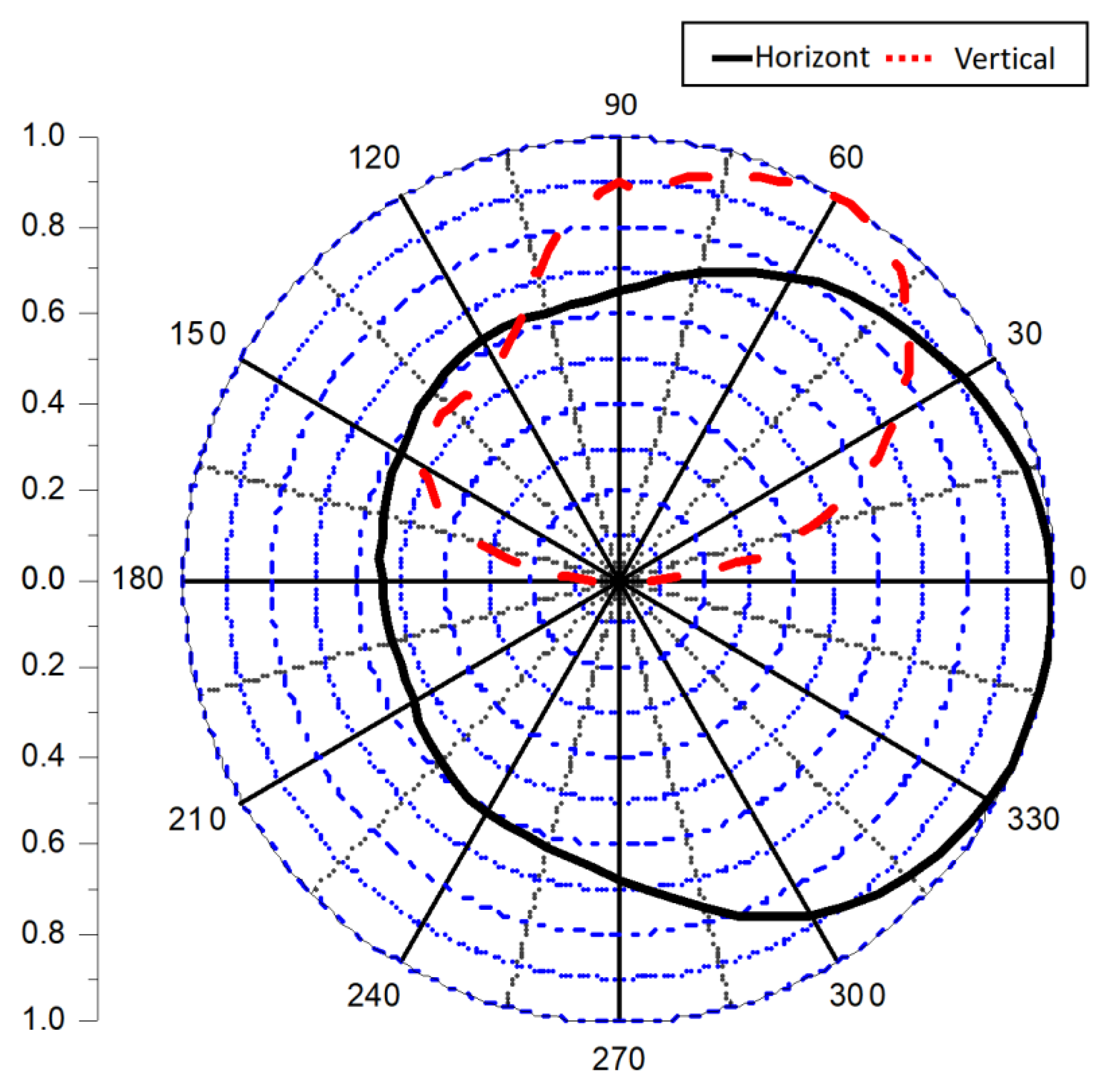
Equipment Modeling: Shortwave interference equipment parameters, such as antenna dimensions, maximum gain, and standing wave ratio, are inputted through a user-friendly visual interface. The antenna patterns at various frequencies were then established based on the specified parameters.

(2)

Determining Transmission and Reception Positions: The equipment’s deployment position serves as the emission point for the interference signal, while the calculation of the received field strength at the interference footprint is designated as the receiving point.

(3)

Calculating the Grid Matrix: A grid link was established to facilitate precise calculations using the interference impact area grid matrix method.

(4)

Analyzing Ionospheric Parameters: Simulating the state of the ionosphere in the assessment area involves employing an ionospheric parameter model. This model considers factors such as the ionospheric height, density distribution, and electron density to determine the ionospheric state based on temporal and spatial variations.

(5)

Matching Antenna Pattern: Selecting the emission frequency of the device prompts an automatic match with the corresponding antenna pattern or the closest antenna pattern within the established set.

(6)

Propagation Prediction: Employing the ITU-R P.533-14 wave propagation model, the simulation of shortwave signal propagation in the ionosphere incorporates reflection, refraction, and scattering characteristics across different frequency bands. The model calculates the signal’s propagation path in the ionosphere based on ionospheric parameters and emission signal frequency, determining interference strength at each grid link’s fall point.

(7)

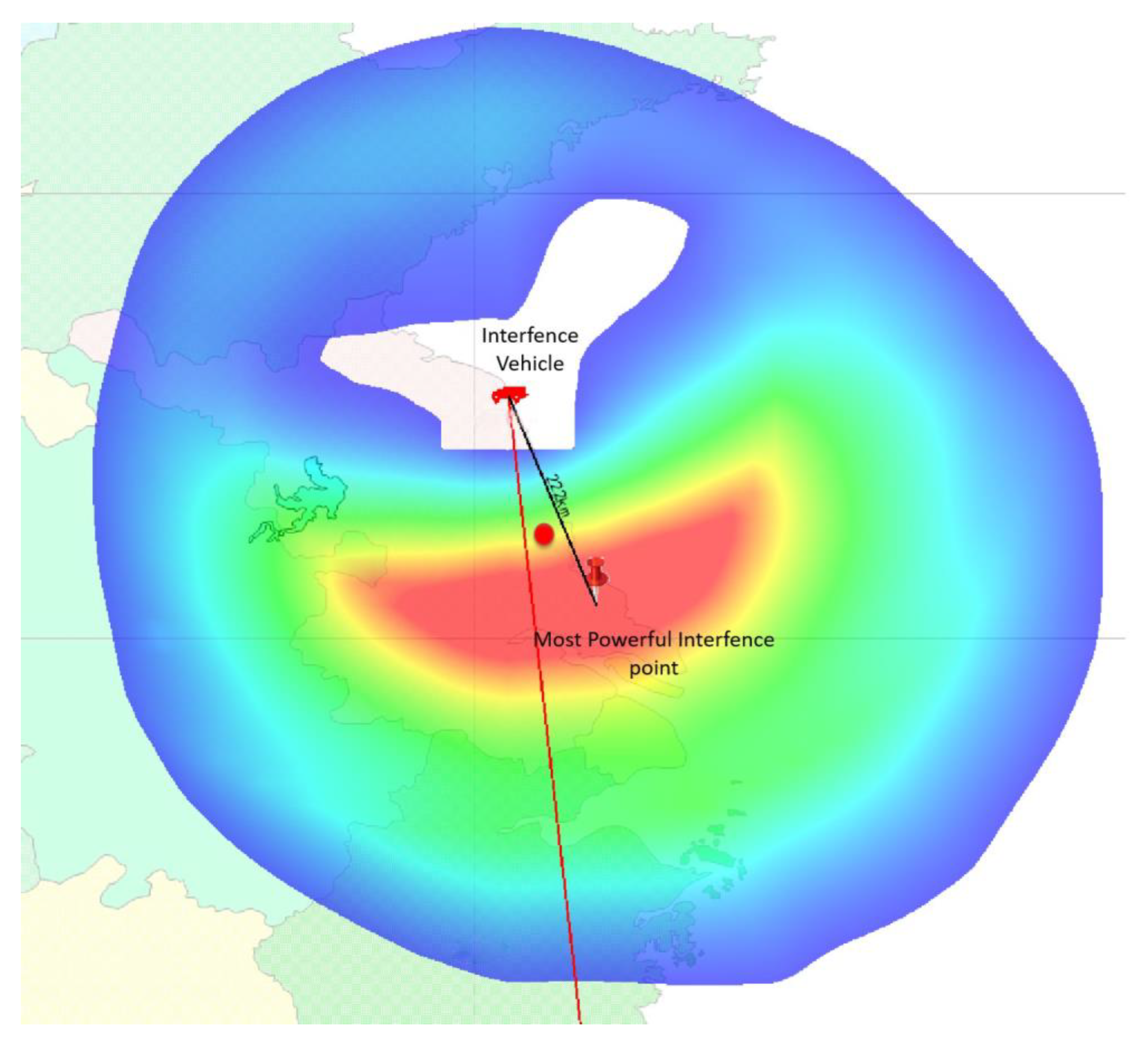
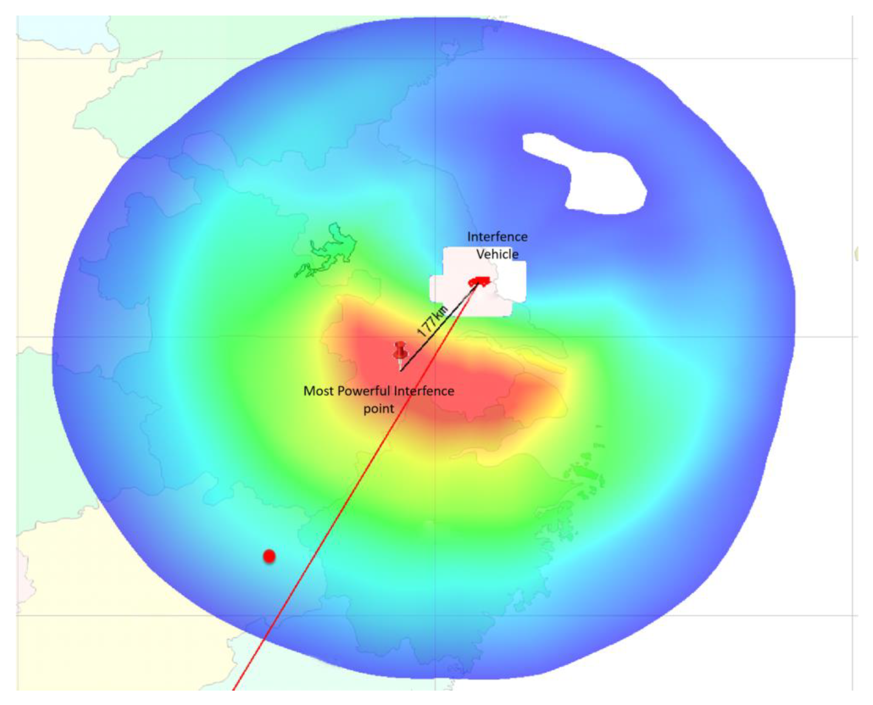
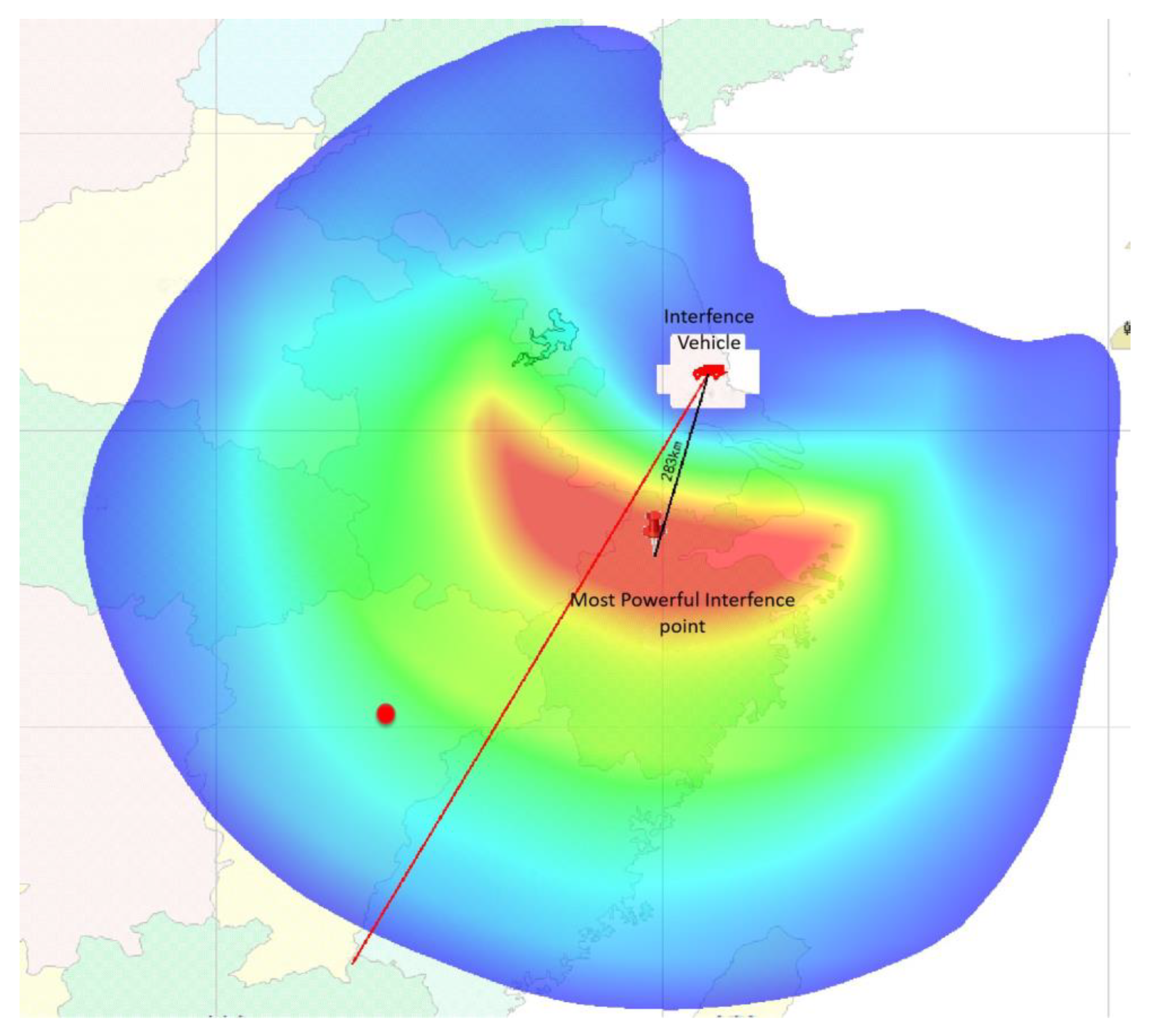
Visualization: Setting an interference strength threshold enables the visualization of the interference footprint based on the grid interference strength. Grid points below the threshold were not excluded from the visualization process.

Based on the above principles of operation, we can use the above tools to predict the interference range and intensity of the shortwave interference signals. We deployed shortwave interference vehicles at points (120.59, 32.35) and (120.59, 32.35), with antenna azimuth pointing at 174°, 213°, 214°, frequencies of 5 MHz, 7 MHz, 9 MHz, power of 10 kW, and test reception points at (120.59, 32.35), (117.51, 28.48), and (116.57, 27.41). A visual image of the interference area can be obtained through the simulation, which displays the range and intensity distribution of the shortwave interference signal, as shown in Figure 5, Figure 6 and Figure 7 [19]. It is crucial for analyzing and formulating strategies for electronic countermeasures and interference, improving the anti-interference capability of communication systems, and ensuring the reliability and security of communication.

We can use this tool to compute the interference impact range and intensity distribution maps of the three links. By selecting the latitude and longitude of the landing points on the map with the mouse, we were able to retrieve the field strength values for the three landing points.

4. Experiment and Verification

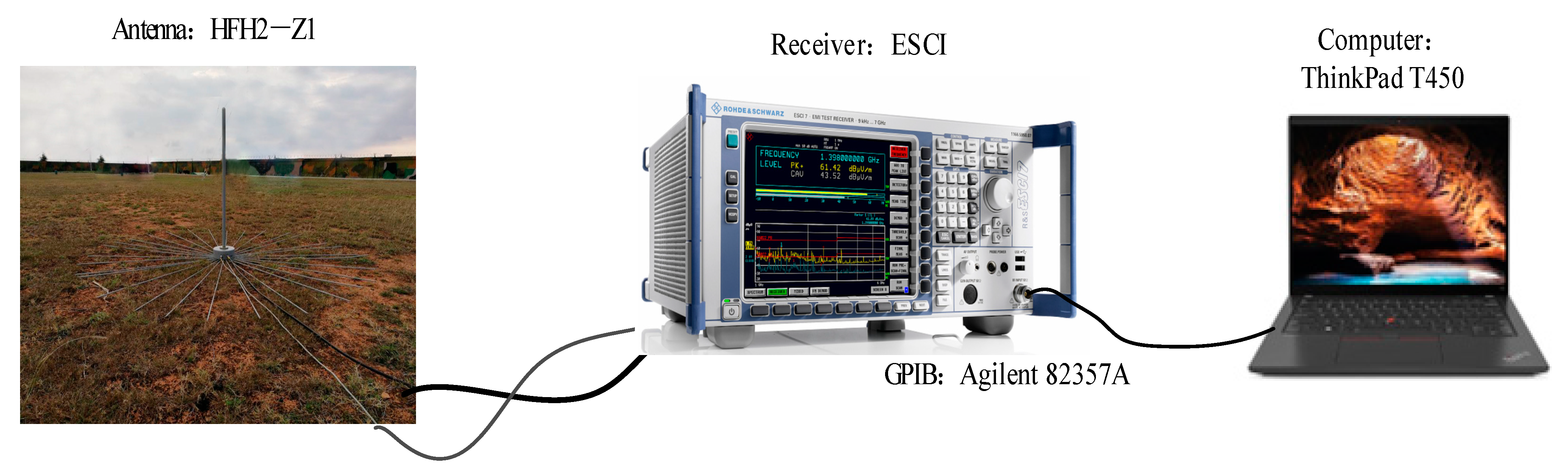
4.1. Experimental Receiving Equipment

The equipment for the experimental receiving systems included a receiving antenna, receiver, general-purpose interface bus card, and computer. The equipment used for the experimental receiving system is listed in

Table 3. List of Experimental Receiving System Equipment.

Equipment Name	Manufacturer	Type	Function
EMI Receiver	R&S	ESCI	Capture and analyze EMI signals.
Standard Rod Antenna	R&S	HFH2-Z1	Receive short-distance signal
Computer	Lenovo	ThinkPad T450	Display monitoring data
GPIB card	Agilent	82357A	Connecting receiver and computer for data transfer and control

.

4.2. Experimental Receiving System Connection

Thick and thin cables link the Standard Rod antenna and R&S receiver. The primary purpose of the thick cable is to convey the signals the antenna receives to the receiver for processing. Conversely, the thin cable is primarily utilized for the receiver to regulate parameters such as the frequency and bandwidth of the received signals from the antenna. The receiver was interfaced with a laptop by using a GPIB card. The laptop dispatches control commands to the receiver via the GPIB card and the receiver, in turn, transmits processed signals back to the laptop for display through the same GPIB card. Figure 8 illustrates the system connection diagram of the experimental receiving system.

4.3. Experimental Process

From 29 October 2020, to 1 November 2020, interference zone field strength prediction accuracy verification experiments of the shortwave communication interference zone assessment tool were conducted in some Jiangsu and Jiangxi Province regions.

The experimental transmitting system used a solid-state shortwave transmitter, and the transmitting antenna was a logarithmic–periodic antenna. The experimental transmission frequency ranges were 5, 7, and 9 MHz, with a transmission power option of 10 kW. The signal was radiated using sky–wave propagation.

The experimental transmission and reception sites were all selected on flat terrain, with no obvious obstruction around the transmission and reception antennas. Three transmission-reception links were set up for this experiment, as listed in

Table 4. Experimental Procedure Arrangement.

Transmitting Position	Receiving Position	Distance	Azimuth	Date	Test Time	Transmitting Power
(120.32, 34.05)	(120.51, 32.42)	155 km	174°	29 October 2020	16:45	10 kW
(120.59, 32.35)	(117.51, 28.48)	525 km	213°	31 October 2020	08:53	10 kW
(120.59, 32.35)	(117.51, 28.48)	525 km	213°	31 October 2020	10:45	10 kW
(120.59, 32.35)	(117.51, 28.48)	525 km	213°	31 October 2020	15:06	10 kW
(120.59, 32.35)	(116.57, 27.41)	675 km	214°	1 November 2020	10:36	10 kW
(120.59, 32.35)	(116.57, 27.41)	675 km	214°	1 November 2020	17:39	10 kW

.

4.4. Comparison of Experimental Results

For each link, the median of the received signal strength measured at the receiving point was calculated based on the test period and the transmission power. For 3 links, 6 sets of data were measured at 6 different time points over a period of 2.5 days. Each set of data was measured for a duration of approximately 20 min, and the median was calculated for each set of data. The measured median received signal field strength (dBμV/m) results corresponded to the calculated results in

Table 5. Simulated and measured results.

No.	Frequency (MHz)	Measured Position		Simulated Result (dBμV/m)	Measured Result (dBμV/m)
		Latitude (°N)	Longitude (°E)
1.	5.000	32.35	120.59	48	39.23
2.	7.000	28.48	117.51	41	30.39
3.	7.000	28.48	117.51	39	30.34
4.	7.000	28.48	117.51	36	28.68
5.	9.000	27.41	116.57	43	36.92
6.	9.000	27.41	116.57	48	38.82

in the experiment.

This experiment was based on the location of the transmission and reception points of three links, lasting for 2.5 consecutive days, including the afternoon of 29 October, the entire day of 31 October, and the entire day of 1 November 2020. We measured the propagation field strength at 5 MHz, 7 MHz, and 9 MHz using the statistical median of received field strength and conducted three measurements. We calculated the errors between the measurement results and the calculation results of the shortwave communication interference assessment software, which are 8.77 dB, 10.61 dB, 8.66 dB, 7.32 dB, 6.08 dB and 9.12 dB, respectively. The mean error is 8.42 dB, whereas the conventional shortwave communication attenuation error typically hovers around 10 dB. This analytical tool effectively mitigated the error by 1.58 dB.

5. Conclusions

We have developed a pioneering tool that revolutionizes the assessment of shortwave communication interference zones caused by shortwave interference devices. This groundbreaking tool seamlessly integrates ionospheric parameters, sunspots, and meteorological data into a comprehensive database that also includes equipment spectral characteristic parameters, radio wave environmental data, and terrain information. Users are empowered to perform crucial management operations, such as adding, deleting, and modifying data in the database and providing unprecedented control and customization.

The focal point of innovation lies in the implementation of cutting–edge algorithms and interfaces, specifically designed to calculate the interference of shortwave interference devices with different antenna types and ionospheric absorption. Rigorous validation through comparative analysis with measured results underpins the exceptional accuracy and reliability of this tool, setting a new standard for precision in interference assessment.

This tool enables us to not only effectively model shortwave interference devices based on their performance parameters, but also to simulate the impact of deploying them at specified locations with unparalleled accuracy and insight. Furthermore, by revealing the interference impact area after shortwave interference devices reflect off the ionosphere, this tool offers invaluable guidance to optimize the effectiveness of device deployment, presenting a transformative shift in strategic decision-making.

Through the exclusive utilization of this tool, users can access unparalleled capabilities to precisely assess and predict the interference impact range of shortwave interference devices, ushering in a new era of informed and effective deployment and implementation strategies.

References

1. Wang, J.; Shi, Y.; Yang, C.; Zhang, Z.; Zhao, L. A Short-Term Forecast Method of Maximum Usable Frequency for HF Communication. IEEE Trans. Antennas Propag. 2023, 71, 5189–5198. [Google Scholar] [CrossRef]
2. Wang, J.; Shi, Y.; Yang, C. An Overview and Prospects of Operational Frequency Selecting Techniques for HF Radio Communication. Adv. Space Res. 2022, 69, 2989–2999. [Google Scholar] [CrossRef]
3. Wang, J.; Yang, C.; An, W. Regional Refined Long-term Predictions Method of Usable Frequency for HF Communication Based on Machine Learning over Asia. IEEE Trans. Antennas Propag. 2022, 70, 4040–4055. [Google Scholar] [CrossRef]
4. Lin, J.; Wang, D.; Yan, C. Research on integrated interference evaluation against HF communication channel. IEEE Access 2018, 6, 61575–61584. [Google Scholar]
5. Wu, L.; Shang, H.; Lü, S. An interference estimation method for shortwave communication system based on wavelet packet transform and support vector regression. J. Appl. Remote Sens. 2017, 11, 035013. [Google Scholar]
6. Kumar, A.; Singh, S.P.; Garg, P.K. HF radio wave propagation analysis in the presence of interference using generalized regression neural network. J. Atmos. Sol. Terr. Phys. 2018, 177, 137–147. [Google Scholar]
7. Kaushik, H.S.; Bhattacharya, B.K.; Balakrishnan, R. Simplified models for ionospheric scintillation effects on HF radio communication in the equatorial ionosphere. J. Atmos. Sol. Terr. Phys. 2019, 193, 105058. [Google Scholar]
8. Lee, H.Y.; Uhm, M.S.; Lee, G.S. Interference mitigation techniques for shortwave radios. J. Commun. Netw. 2018, 20, 609–625. [Google Scholar]
9. Kim, D.; Lee, C.; Kim, J. Analysis of interference on high frequency communication systems using HF diplex filters. J. Electrostat. 2017, 88, 104–110. [Google Scholar]
10. Liu, L.; Liu, Y.; Sun, J. A method for the suppression of interference in shortwave communication systems based on the grey wolf optimization algorithm. Measurement 2017, 98, 115–124. [Google Scholar]
11. Dorji, U.; Kim, G.H.; Kim, J.H.; Bak, K.H. Development of a compact HF channel sounder for shortwave radio communications in low-latitude regions. Meas. Sci. Technol. 2020, 31, 064003. [Google Scholar]
12. Ahmed, S.M.; Nasr, M.S.; El Sayed, M.A. Radio communication interference in tropical regions: Model development and analysis. J. Atmos. Sol. Terr. Phys. 2017, 163, 118–129. [Google Scholar]
13. Mestan, M.; Ertugrul, N. Interference analysis of a shortwave communication system by using a psychoacoustic-based speech quality measure. Int. J. Electr. Eng. 2016, 16, 35–41. [Google Scholar]
14. Kaneko, Y.; Ogawa, T.; Ikeda, K. HF interference effects on IQ data of software-defined radios. Radio Sci. 2016, 51, 2198–2208. [Google Scholar]
15. Pan, X.; Wei, G.; Wan, H.; Lu, X.; Li, W.; Wang, Y. Prediction model of blocking interference effects for electronic equipment under the condition of the dual-frequency narrow spectrum in-band electromagnetic radiation. Chin. J. Radio Sci. 2020, 35, 377–385. [Google Scholar] [CrossRef]
16. Du, H.; Yu, Y.; Du, B. Evaluation method of complex electromagnetic environment adaptability for communication station. Chin. J. Radio Sci. 2018, 33, 619–623. [Google Scholar] [CrossRef]
17. International Telecommunication Union (ITU). Recommendation P.1239-2: Characteristics of the Ionosphere-Propagation Data Required for the Design of HF Systems; International Telecommunication Union (ITU): Geneva, Switzerland, 2007. [Google Scholar]
18. ITU-R. Method for the Prediction of the Performance of HF Circuits, ITU-R P.533-14; International Telecommunication Union: Geneva, Switzerland, 2017. [Google Scholar]
19. Watt, A.; Watt, M. 3D Computer Graphics, 4th ed.; Pearson Education Limited: Beijing, China, 2017. [Google Scholar]
Figure 1. System architecture.
Atmosphere 14 01728 g001
Figure 2. The directional pattern of the logarithmic periodic antenna at 5 MHz.
Atmosphere 14 01728 g002
Figure 3. The directional pattern of the logarithmic periodic antenna at 7 MHz.
Atmosphere 14 01728 g003
Figure 4. The directional pattern of the logarithmic periodic antenna at 9 MHz.
Atmosphere 14 01728 g004
Figure 5. Interference Range and Intensity Distribution Map at 5 MHz at 16:45, 29 October 2020.
Atmosphere 14 01728 g005
Figure 6. Interference Range and Intensity Distribution Map at 7 MHz at 10:45, 29 October 2020.
Atmosphere 14 01728 g006
Figure 7. Interference Range and Intensity Distribution Map at 9 MHz at 10:36 29 October 2020.
Atmosphere 14 01728 g007
Figure 8. The experimental receiving–system connection diagram.
Atmosphere 14 01728 g008