Abstract
To improve the accuracy of predicting the ionospheric critical frequency of the F2 layer (foF2), a reconstruction method for the spatial map of the ionospheric foF2 based on modified geomagnetic dip coordinates is proposed. Based on the strong correlation between the ionospheric foF2 and geomagnetic coordinates, the variation function of ionospheric distance is built. In the end, the spatial map of the ionospheric foF2 is predicted by solving the Kriging equation. The results show that the regional characteristics of the ionospheric foF2 analyzed by the proposed method are consistent with the observations. Compared with the reconstructed value of foF2 using traditional geographic coordinates, the root-mean-square error (RMSE) in high solar activity years decreased by 0.43 MHz, and the relative RMSE decreased by 5.48%; The RMSE decreased by 0.35 MHz during low solar activity which is 5.99% lower to relative RMSE. The research results provide support for high-frequency communication frequency selection.
1. Introduction
The ionosphere is the ionized portion of the upper atmosphere (the thermosphere, part of the mesosphere, and the exosphere). It extends from about 60 to beyond 1000 km and completely encircles the Earth. The primary plasma source for the ionosphere is the photoionization of neutral molecules via solar EUV and soft X-ray radiation, although other production processes may dominate in certain regions. The ions produced undergo chemical reactions with the neutrals, recombine with the electrons, diffuse to higher or lower altitudes, or are transported via neutral wind effects []. According to the vertical distribution characteristics of electron density, the ionosphere can be divided into D, E, and F layers, of which the F layer is usually divided into the F1 layer and the F2 layer.
The ionosphere is a time-varying dispersion channel, which varies with seasons, day and night, and regions and is affected by space environments such as solar activity and geomagnetic fields. High-frequency communications are affected by the ionosphere [,]. The ionospheric plasma structure on a wide range of space and time scales can have a destructive impact on space application systems (such as navigation and communication systems operated by Global Navigation Satellite Systems (GNSS)) [], and its spatiotemporal dynamic changes lead to fluctuations in communication channels, which directly affect the reliability and stability of ionospheric communication, this is also the reason why the ionosphere and its communication research has become a research hotspot in the past hundred years []. Existing research also shows that the trend scenario of the ionosphere is now more complete than before, but some gaps and differences still need to be further studied [].
The critical frequency of the F2 layer (foF2), which represents the minimum frequency of electromagnetic waves that can penetrate the ionosphere vertically, is one of the critical parameters of the ionosphere and can be used to understand ionospheric dynamics and structure [], as well as the influence of ionospheric weather on communication and navigation []. foF2 has an irregular and non-uniform spatial distribution, and the unknown data in adjacent regions can be interpolated or extrapolated from the limited known ionospheric observations. This regional ionospheric reconstruction problem is critical in regional ionospheric reporting and prediction [].
Many organizations and scholars have been continuously studying ionospheric regional reconstruction technology for a long time. At present, the ionospheric spatial features description methods based on different empirical or mathematical methods include inverse distance weight (IDW) interpolation [], spline interpolation [], spherical harmonic function [,], neural network (NN) [], deep learning (DL) [], and Kriging method []. Among them, the IDW method lacks the geophysical mechanism and is far from the observation station, so the accuracy is low. The spherical Lagrange function is only orthogonal on the whole sphere and cannot effectively represent the signal in the restricted region on the sphere []. Green function is the most robust, efficient, and accurate method []. The surface spline interpolation based on the green function has good approximation performance. Due to its high accuracy, simplicity, flexibility, and other advantages, it has become the mainstream method and a potent tool for multivariate approximation [].
To achieve high-accuracy regional ionospheric foF2 reconstruction, a new foF2 reconstruction method for the Australian region is proposed by introducing geomagnetic coordinates and improving the Kriging method. In the proposed method, the variation function of ionospheric distance is determined based on geomagnetic coordinates, and the estimated value is obtained by solving the improved Kriging equation. The proposed method is validated and analyzed by using the data collected from 7 ionospheric stations in Oceania.
2. Reconstruction Method
The Kriging method is a widely used interpolation algorithm in ionospheric parameter reconstruction, which can provide the best linear unbiased estimation and accurately describe the spatial structure of ionospheric parameters.
When using the Kriging interpolation method for reconstruction, the variation function is first determined to obtain the spatial autocorrelation of variables, the statistical correlation between observations is estimated, and then the target location []. The reconstructed result of the Kriging model based on MGD coordinates is defined as the linear weighting of the value of the known ionospheric sampling observations (such as foF2), and the formula is as follows:
where, oF2 is the foF2 reconstruction value of any location, N is the maximum number of observation stations, wn is the weight coefficients of the nth observation station, foF2(λn, φn) is the observation value of the nth station, λn and φn are the latitude and longitude of the nth observation station respectively.
The Lagrange multiplier algorithm is used to calculate the weight coefficients. To make the mathematical expectation of the error of the estimated value of foF2(λ, φ) zero and to minimize the sum of squares between the reconstructed value and the observed value, the optimal weight coefficients wn can be solved from the linear Kriging equation []:
where, N is the maximum number of observation stations used for spatial interpolation, μ is the Lagrange factor, rij is the ionospheric distance between stations i and j, ri0 is the ionospheric distance between station i and the reconstructed station, and the sum of all weight coefficients is 1 to ensure the unbiased reconstruction results:
The above process is the reconstruction of the ionospheric parameter. Its core is to use the variation function established by ionospheric distance to find the spatial correlation, determine the weight coefficients of each ionospheric observation station, and finally solve the reconstructed value of the target location by a linear combination of the known observed value and the calculated weight coefficients [].
In the current common reconstruction methods, the ionospheric distance is mostly calculated using the modified Euclidean distance with scale factor (SF) in the standard geographic coordinate system, which is the ionospheric distance determined by Stanislawska when he introduced the Kriging interpolation method into the ionospheric field []. Considering that the ionosphere is jointly controlled by the direction of the Earth’s rotation axis and the geomagnetic field structure, geomagnetic parameters play an important role in the main variations of the ionosphere, especially in the F2 layer, and the variation trend of the F2 layer parameters is strongly correlated with geomagnetic coordinates []. Therefore, the model no longer adopts simple traditional geographical coordinates (TGG), but geomagnetic coordinates can be adopted. Modified geomagnetic dip coordinates (MGD) have been proven to be very effective in modeling ionospheric parameters, especially suitable for the ionospheric F2 layer plasma characteristics [,,]. Therefore, the ionospheric distance is determined based on the MGD as follows:
where, (ϑi, ϕi) and (ϑj, ϕj) correspond to the geomagnetic longitude and latitude of the ith position (λi, φi) and the jth position (λj, φj) respectively; s is the scale factor, reflecting the different variations of ionospheric parameters in the specific region at the magnetic longitude and latitude.
In summary, the specific implementation process of the above reconstruction method is as follows: Based on the determined ionospheric distance calculation method, the semi-variation function of the ionospheric distance between observation stations is estimated:
At the same time, the ionospheric distance vector between the unknown location (λi, φi) and the known observation station (λ0, φ0) can be calculated, including the semi-variation function (R0):
Formulas (2) and (3) are used to calculate the weight coefficients W, which is expressed by vector representation:
Finally, the ionospheric parameters at any position are calculated using Equation (1).
3. Method Validation
The foF2 used in this paper can be obtained from the ftp://ftp-out.sws.bom.gov.au/wdc/iondata/medians (accessed on 1 May 2023), which contains ionospheric monthly medians obtained from manually scaled hourly ionospheric data. The seven stations selected in Australia are Brisbane, Canberra, Learmonth, Perth, Darwin, Townsville, and Hobart. Figure 1 shows the geographical and geomagnetic location distributions of the stations. Table 1 shows the station’s corresponding geographical and geomagnetic coordinates, where the expressions of geomagnetic latitude and modified geomagnetic dip longitude are shown in Equation (8) and Equation (9), respectively:
(a) geomagnetic latitude []:
where λm is geomagnetic latitude, λ and φ are the geographic latitude and longitude, respectively, of the apex, and λ0 and φ0 are the geographic latitude and longitude, respectively, of the north pole of the earth-centered dipole.
(b) Modified Geomagnetic Dip []:
where I is the magnetic dip angle, defined by the downward and horizontal components of the field, and λ is geographical latitude.
(c) Modified Geomagnetic Dip Longitude []:
where μ is the modified geomagnetic dip angle, λm is the geomagnetic latitude, φ is the geographic longitude of the apex, and φ0 is the geographic longitude of the north pole of the earth-centered dipole.
It can be seen from the Figure 1 as follows:
(1) The spatial distribution of the MGD coordinates is significantly different from that of the TGG coordinates;
(2) The geomagnetic longitude marked by the blue line has a specific deviation from the geographical longitude line, and the greater the deviation is toward the east;
(3) The modified geomagnetic dip latitude marked by the red line significantly differs from the geographical latitude, especially in the low and high-latitude regions.
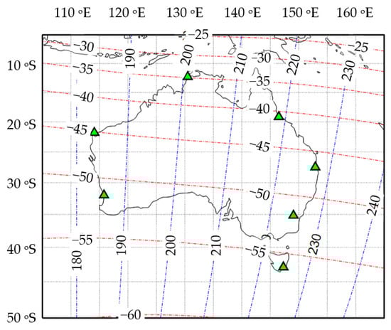
Figure 1.
Location distribution of ionospheric observation stations in geographic coordinates and different geomagnetic coordinates.

Table 1.
The different coordinates of the ionospheric observation station.
Table 1.
The different coordinates of the ionospheric observation station.
| Label | Station | TGG | MGD | ||
|---|---|---|---|---|---|
| Latitude (°N) | Longitude (°E) | Geomagnetic Latitude (°N) | Modified Geomagnetic Dip Longitude (°E) | ||
| 1 | Brisbane | −27.50 | 152.90 | −46.85 | 227.14 |
| 2 | Canberra | −35.17 | 149.07 | −51.85 | 224.68 |
| 3 | Darwin | −12.28 | 130.50 | −34.81 | 200.84 |
| 4 | Hobart | −42.90 | 147.30 | −56.05 | 224.85 |
| 5 | Learmonth | −21.80 | 114.10 | −45.13 | 183.46 |
| 6 | Perth | −32.00 | 115.80 | −51.58 | 185.66 |
| 7 | Townsville | −19.15 | 146.50 | −40.87 | 218.73 |
To estimate the influence of different coordinates and different distance SFs on the reconstruction results, root-mean-square error (RMSE) and relative root-mean-square error (RRMSE) are selected as the evaluation criteria of the proposed method, and the formula is as follows:
- (a)
- RMSE:
- (b)
- RRMSE:
For the stations shown in Figure 1, based on the MGD and the observed foF2 values of the seven ionospheric stations from 2013 to 2017, different distance SFs s were analyzed, and the reconstructed RMSEs were shown in Figure 2a below. It can be seen that the RMSE decreases gradually and then increases slightly as the SF s increases. When the s is 9.5, the RMSE is the smallest, so the optimal SF is determined. In this case, the corresponding ionospheric distance is shown in Figure 2b, which fundamentally differs from the traditional distance.
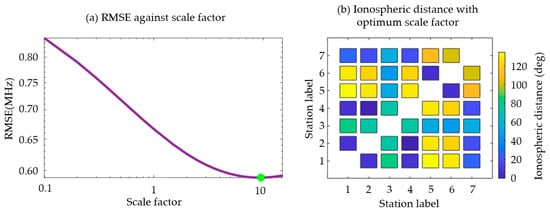
Figure 2.
The optimal scale factor and its corresponding ionospheric distance distribution.
According to the optimal SF determined above, the foF2 in the Oceania region is reconstructed. The typical reconstruction diagram is shown in the following Figure 3.
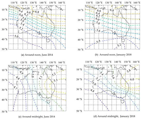
Figure 3.
Reconstructions around noon and midnight in high solar activity years (June 2014) and low solar activity years (January 2018): (a) 3:00 UTC (around noon), June 2014, high solar activity year; (b) 3:00 UTC (around noon), June 2018, low solar activity year; (c) 15:00 UTC (around noon), June 2014, high solar activity year; (d) 15:00 UTC (around noon), June 2018, low solar activity year.
As can be seen from Figure 3, the maximum value appears near the equator, and the foF2 gradually decreases with the increase of latitude. With the change of time, the maximum value region has a drift property near the equator, and the drift property is the same in different years. Generally, the foF2 of noon is higher than the value of midnight, and the foF2 of high solar activity is higher than that of low solar activity. These characteristics are consistent with the trend of ionospheric characteristics in the southern hemisphere, proving this method’s effectiveness and applicability.
Further, according to the observation data of the seven stations, the cross-validation method was adopted to reconstruct the 24-h foF2 of the seven stations one by one and analyze the error. The following Figure 4 shows the comparison between the observed values and the reconstructed values at noon in low solar activity years (a~g) and high solar activity years (h~n).
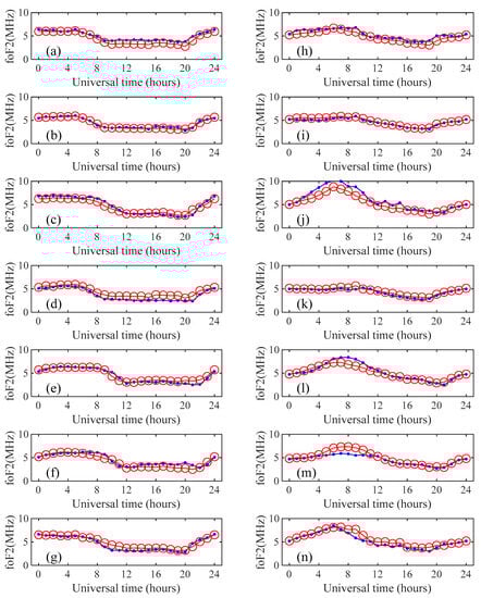
Figure 4.
Comparison of 24 h observed and reconstructed results. (a–g) is the result during June 2014 at the Brisbane, Canberra, Darwin, Hobart, Learmonth, Perth, and Townsville; (h–n) is the result during January 2014 at the Brisbane, Canberra, Darwin, Hobart, Learmonth, Perth, and Townsville. Blue dot lines are observed values, and red circle lines are reconstructed values.
In Figure 4, the left column is the comparison of the high solar activity year, and the right column is the comparison of the low solar activity year. It can be seen from Figure 4 that the reconstruction accuracy of Canberra, Darwin, and Learmonth stations in low solar activity years is the highest. The observed results are consistent with the reconstruction results. In contrast, the reconstruction accuracy of other stations at night will show slight deviations, and the reconstruction results in other periods are consistent with the observed values. In high solar activity years, the reconstruction results of Brisbane, Canberra, Hobart, and Townsville stations have high accuracy, while the other stations have certain deviations around noon, and the reconstruction results of other times are relatively accurate. Combining the above two groups of curves, the period with high reconstruction accuracy accounted for 81.9%, and the period with slight deviation accounted for 18.1%.
To further illustrate the advantages of using the Kriging method based on TGG coordinates (Kriging-TGG) for ionospheric foF2 modeling, we compare the results with those based on MGD coordinates (Kriging-MGD). Figure 5a shows the ionospheric distance calculated using TGG coordinates. Figure 5b shows the absolute value of the difference between the ionospheric distance calculated using MGD coordinates and the ionospheric distance calculated using TGG coordinates, which shows a particular gap in the ionospheric distance calculated under the two different coordinates.
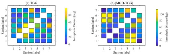
Figure 5.
Ionospheric distance: (a) The ionospheric distance is calculated using TGG coordinates. (b) The absolute value of the difference between the ionospheric distance was calculated using MGD coordinates, and the ionospheric distance was calculated using TGG coordinates.
To measure the performance of the two Kriging methods, more specifically, the RMSE and RRMSE of the two methods are calculated respectively according to Equations (11) and (12).
Figure 6 and Figure 7 show the RMSE in summer when solar activity is high and winter when solar activity is low, respectively. Among them, the hollow circle is the RMSE obtained by the Kriging-TGG, and the solid circle is the RMSE obtained by the Kriging-MGD. The size or color of the circle can represent the size of the RMSE. For any station, the RMSE obtained using the Kriging-MGD is smaller than that obtained using the Kriging-TGG.
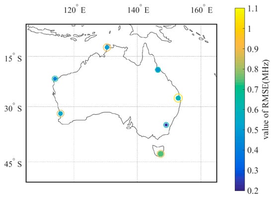
Figure 6.
RMSE obtained by two Kriging models in summer when solar activity is high.
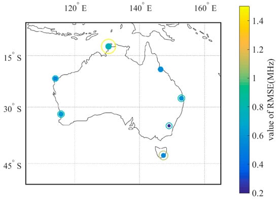
Figure 7.
RMSE obtained by two Kriging models in winter when solar activity is low.
Figure 8 shows the difference in RMSE statistically obtained using the two Kriging models, with the horizontal axis representing the size of RMSE and the vertical axis representing the station name. The length of the green column represents the difference in RMSE when the solar activity is high in summer, which shows that the difference in RMSE between the two Kriging models is 0.43 MHz at the maximum and 0.16 MHz at the minimum. The length of the red column represents the difference in RMSE in winter when the solar activity is low, which shows that the difference in RMSE between the two models at Darwin station is the largest, 0.71 MHz. The difference in RMSE between the two models at Townsville station is the smallest, 0.03 MHz. Using the Kriging-TGG, the average RMSE of the seven stations is 0.81 MHz when the solar activity is high in summer and 0.90 MHz when the solar activity is low in winter. Using the Kriging-MGD, the average RMSE of the seven stations is 0.50 MHz when the solar activity is high in summer, and the average RMSE in winter when solar activity is low is 0.55 MHz, which decreases by 0.31 MHz and 0.71 MHz, respectively, compared with the Kriging-TGG coordinates.
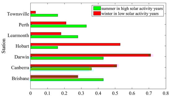
Figure 8.
The difference between the RMSE reconstructed based on the Kriging-TGG and the RMSE reconstructed based on the Kriging-MGD.
Figure 9 shows the RRMSE obtained statistically using two Kriging models. The cylinder’s length represents the RRMSE’s size, and the blue circle corresponds to the right vertical axis, representing the difference between the RRMSE obtained statistically by the Kriging-TGG and the RRMSE obtained statistically by the Kriging-MGD. Figure 9a shows the statistical diagram of RRMSE in high summer solar activity years, which shows that for any station, the RRMSE obtained by the Kriging-MGD is smaller than that obtained by the Kriging-TGG. The difference in RRMSE of the Hobart station is the smallest, while that of the Brisbane station is the largest. Figure 9b shows the statistical diagram of RRMSE in winter low solar activity years. Except for the Townsville station, the RRMSE obtained by the Kriging-MGD is smaller than that obtained by the Kriging-TGG. The RRMSE obtained by the Kriging-MGD is 1.33% larger than that obtained by the Kriging-TGG.
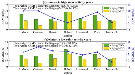
Figure 9.
RRMSE obtained by two Kriging methods: (a) summer when solar activity is high (b) winter when solar activity is low.
Generally, the average RRMSE of the seven stations is 19.98% in summer when the solar activity is high, 18.81% in winter when the solar activity is low, and 14.50% in summer when the Kriging-MGD is applied. The average RRMSE in winter when solar activity is low is 12.82%; compared with the Kriging-TGG, RRMSE decreased by 5.48% and 5.99%, respectively.
According to the above analysis, the Kriging-MGD has advantages over the Kriging-TGG. In other words, using geomagnetic coordinates instead of geographic coordinates to calculate ionospheric distance can realize ionospheric foF2 reconstruction with higher accuracy.
4. Conclusions
In this paper, by introducing modified geomagnetic dip coordinates, we proposed a high-accuracy foF2 regional reconstruction model over the Australian region. The regional characteristics are consistent with the objective characteristics of the ionosphere, and the results can reflect the physical characteristics of ionospheric foF2 at different locations. In addition, we compared the Kriging-MGD with the Kriging-TGG. The experimental results show that the mean RMSE and RRMSE of Kriging-MGD are 0.50 MHz and 14.50%, respectively, in summer when solar activity is high. The RMSE and RRMSE of Kriging-TGG are 0.81 MHz and 19.98% respectively. When solar activity is low in winter, the average RMSE and RRMSE of Kriging-MGD and Kriging-TGG are 0.55 MHz and 12.82%, respectively, and 0.90 MHz and 18.81%, respectively. The results show that compared with Kriging-TGG, Kriging-MGD has more minor errors and higher accuracy. This technology can be extended to the global region and provide essential support for optimizing long-distance communication systems’ frequency.
Author Contributions
Conceptualization, Y.L., Q.Y., Y.S., C.Y. and J.W.; methodology, Y.L., Q.Y., Y.S., C.Y. and J.W.; software, Y.L., Q.Y., Y.S. and C.Y.; validation, Y.L., Q.Y., Y.S., C.Y. and J.W.; formal analysis, C.Y. and J.W.; investigation, Y.L., Q.Y., Y.S., C.Y. and J.W.; resources, J.W. and C.Y.; data curation, Y.L. and J.W.; writing—original draft preparation, Y.L., Q.Y. and Y.S.; writing—review and editing, Y.L., Q.Y., Y.S., C.Y. and J.W.; visualization, Y.L., Q.Y. and Y.S.; project administration, C.Y. and J.W.; funding acquisition, C.Y. and J.W. All authors have read and agreed to the published version of the manuscript.
Funding
This research was funded by the National Natural Science Foundation of China (No. 62031008) and the State Key Laboratory of Complex Electromagnetic Environment Effects on Electronics and Information Systems (No. CEMEE2022G0201, CEMEE-002-20220224).
Institutional Review Board Statement
Not applicable.
Informed Consent Statement
Not applicable.
Data Availability Statement
Not applicable.
Conflicts of Interest
The authors declare no conflict of interest.
References
- Schunk, R.; Nagy, A. Ionospheres: Physics, Plasma Physics, and Chemistry; Cambridge University Press: Cambridge, UK, 2009. [Google Scholar]
- Wang, J.; Yang, C.; An, W. Regional Refined Long-Term Predictions Method of Usable Frequency for HF Communication Based on Machine Learning Over Asia. IEEE Trans. Antennas Propag. 2022, 70, 4040–4055. [Google Scholar] [CrossRef]
- Wang, J.; Shi, Y.; Yang, C.; Zhang, Z.; Zhao, L. A Short-Term Forecast Method of Maximum Usable Frequency for HF Communication. IEEE Trans. Antennas Propag. 2023, 71, 5189–5198. [Google Scholar] [CrossRef]
- Mandea, M.; Korte, M.; Yau, A.; Petrovsky, E. Geomagnetism, Aeronomy and Space Weather; Cambridge University Press: Cambridge, UK, 2019. [Google Scholar]
- Wang, J.; Shi, Y.F.; Yang, C.; Feng, F. A Review and Prospects of Operational Frequency Selecting Techniques for HF Radio Communication. Adv. Space Res. 2022, 69, 2989–2999. [Google Scholar] [CrossRef]
- Laštovička, J. Global pattern of trends in the upper atmosphere and ionosphere: Recent progress. J. Atmos. Sol. Terr. Phys. 2009, 71, 1514–1528. [Google Scholar] [CrossRef]
- Atıcı, R.; Pala, Z. Prediction of the Ionospheric foF2 Parameter Using R Language Forecasthybrid Model Library Convenient Time Series Functions. Wirel. Pers. Commun. 2022, 122, 3293–3312. [Google Scholar] [CrossRef]
- Rao, T.V.; Sridhar, M.; Ratnam, D.V.; Harsha, P.B.S.; Srivani, I. A Bidirectional Long Short-Term Memory-Based Ionospheric foF2 and hmF2 Models for a Single Station in the Low Latitude Region. IEEE Geosci. Remote Sens. Lett. 2022, 19, 8005405. [Google Scholar] [CrossRef]
- Liu, R.Y.; Liu, G.H.; Wu, J.; Zhang, B.C.; Huang, J.Y.; Hu, H.Q.; Xu, Z.H. Ionospheric foF2 reconstruction and its application to the short-term forecasting in China region. Chin. J. Geophys. 2008, 51, 300–306. (In Chinese) [Google Scholar] [CrossRef]
- Pradipta, R.; Valladares, C.E.; Carter, B.A.; Doherty, P.H. Interhemispheric propagation and interactions of auroral traveling ionospheric disturbances near the equator. J. Geophys. Res. Space Phys. 2016, 121, 2462–2474. [Google Scholar] [CrossRef]
- Sandwell, D.T. Biharmonic spline interpolation of GEOS-3 and SEASAT altimeter data. Geophys. Res. Lett. 1987, 14, 139–142. [Google Scholar] [CrossRef]
- Jones, W.B.; Gallet, R.M. Representation of diurnal and geographic variations of ionospheric data by numerical methods. Telecomm. J. 1962, 29, 129–147. [Google Scholar] [CrossRef]
- Chen, L.J.; Zhen, W.M.; Ou, M.; Yu, X.; Song, F.L. A method of ionospheric foF2 reconstruction in low and middle latitudes of the world based on stepwise linear optimal estimation. Chin. J. Radio Sci. 2021, 36, 36–42. (In Chinese) [Google Scholar]
- Verkhoglyadova, O.; Maus, N.; Meng, X. Classification of High Density Regions in Global Ionospheric Maps With Neural Networks. Earth Space Sci. 2021, 8, e2021EA001639. [Google Scholar] [CrossRef]
- Chen, Z.; Jin, M.; Deng, Y.; Wang, J.; Huang, H.; Deng, X.; Huang, C. Improvement of a Deep Learning Algorithm for Total Electron Content Maps: Image Completion. J. Geophys. Res. Space Phys. 2019, 124, 790–800. [Google Scholar] [CrossRef]
- Huang, L.; Zhang, H.; Xu, P.; Geng, J.; Wang, C.; Liu, J. Kriging with Unknown Variance Components for Regional Ionospheric Reconstruction. Sensors 2017, 17, 468. [Google Scholar] [CrossRef] [PubMed]
- Alice, P.B.; Zubair, K.; Rodney, A.K. Slepian Spatial-Spectral Concentration Problem on the Sphere: Analytical Formulation for Limited Colatitude–Longitude Spatial Region. IEEE Trans. Signal Process. 2016, 65, 1527–1537. [Google Scholar]
- Boer, A.D.; Zuijlen, A.H.V.; Bijl, H. Advanced Computational Methods in Science and Engineering—Radial Basis Functions for Interface Interpolation and Mesh Deformation; Springer: Berlin, Germany, 2009. [Google Scholar]
- Smith, M.J.; Cesnik, C.E.S.; Hodges, D.H. Evaluation of Some Data Transfer Algorithms for Noncontiguous Meshes. J. Aerosp. Eng. 2000, 13, 52–58. [Google Scholar] [CrossRef]
- Jiang, C.; Zhou, C.; Liu, J.; Lan, T.; Yang, G.B.; Zhao, Z.Y.; Zhu, P.; Sun, H.Q.; Cui, X. Comparison of the Kriging and neural network methods for modeling foF2 maps over North China region. Adv. Space Res. 2015, 56, 38–46. [Google Scholar] [CrossRef]
- Wang, J.; Bai, H.M.; Huang, X.D.; Cao, Y.B.; Chen, Q.; Ma, J.G. Simplified regional prediction model of long-term trend for critical frequency of ionospheric F2 Region over east Asia. Appl. Sci. 2019, 9, 3219. [Google Scholar] [CrossRef]
- Bowen, Z.; Yuji, Z.; Henkel, P.; Günther, C. Estimation of code ionospheric biases using Kriging method. In Proceedings of the 2015 IEEE Aerospace Conference, Big Sky, MT, USA, 7–14 March 2015. [Google Scholar]
- Stanisκawska, I.; Juchnikowski, G.; Cander, L.R. Kriging method for instantaneous mapping at low and equatorial latitudes. Adv. Space Res. 1996, 18, 217–220. [Google Scholar] [CrossRef]
- Danilov, A.D.; Konstantinova, A.V. Relationship between foF2 trends and geographic and geomagnetic coordinates. Geomagn. Aeron. 2014, 54, 323–328. [Google Scholar] [CrossRef]
- Rawer, K. Geophysics III. In Encyclopedia of Physics; Springer: New York, NY, USA, 1984. [Google Scholar]
- Gustafsson, G.; Papitashvili, N.E.; Papitashvili, V.O. A revised corrected geomagnetic coordinate system for Epochs 1985 and 1990. J. Atmos. Terr. Phys. 1992, 54, 1609–1631. [Google Scholar] [CrossRef]
- Emmert, J.T.; Richmond, A.D.; Drob, D.P. A computationally compact representation of Magnetic-Apex and Quasi-Dipole coordinates with smooth base vectors. J. Geophys. Res. Atmos. 2010, 115, A08322. [Google Scholar] [CrossRef]
- Vanzandt, T.E.; Clark, W.L.; Warnock, J.M. Magnetic Apex Coordinates: A Magnetic Coordinate System for the Ionospheric f 2 Layer; Environmental Research Laboratories: Washington, DC, USA, 1972; Volume 55, p. 77. [Google Scholar]
Disclaimer/Publisher’s Note: The statements, opinions and data contained in all publications are solely those of the individual author(s) and contributor(s) and not of MDPI and/or the editor(s). MDPI and/or the editor(s) disclaim responsibility for any injury to people or property resulting from any ideas, methods, instructions or products referred to in the content. |
© 2023 by the authors. Licensee MDPI, Basel, Switzerland. This article is an open access article distributed under the terms and conditions of the Creative Commons Attribution (CC BY) license (https://creativecommons.org/licenses/by/4.0/).