Article

The Influence of Meteorological Factors and the Time of Day on the Concentration of Ammonia in the Atmosphere Measured Using the Photoacoustic Method near a Cattle Farm—A Case Study

1
Horticultural and Educational Services Beata Kułek, Osiedle Przyjaźni 13/92, 61-687 Poznań, Poland
2
Department of Meteorology, Institute of Geography and Earth Sciences, Eötvös Loránd University (ELTE), Pázmány Péter str. 1/A, H-1117 Budapest, Hungary
*
Author to whom correspondence should be addressed.
Atmosphere 2023, 14(11), 1703; https://doi.org/10.3390/atmos14111703
Submission received: 12 August 2023 / Revised: 23 September 2023 / Accepted: 25 September 2023 / Published: 20 November 2023
(This article belongs to the Special Issue Ammonia Emission and Particulate Matter)

Abstract

:
Influences of animals, time of day, air temperature and relative humidity, wind speed and direction on ammonia concentrations were investigated. A case study on a typical summer day from 7:00 to approximately 24:00 CEST (moderate wind speed, variable cloudiness and maximum global radiation higher than 950 W/m2) in west–central Poland is presented. Concentrations of this gas were measured at four heights (0.1–1.5 m), which were changed every 5 min, using a Nitrolux 1000 photoacoustic spectrometer. A micrometeorological station was established to also measure the surface energy budget components. The results presented are the average for each hour and for the entire day. The fine structure of concentration profiles, plume detection and uncertainty of ammonia flux calculation are also presented. The highest NH3 concentrations were at a 0.5 m height between 16:00 and 17:00 h when cows were grazing, but the lowest concentrations were between 23:00 and 24:00 h at the height of 1.5 m. The ammonia concentration increased with increasing air temperature and was the highest with a westerly wind direction and decreased with increasing air relative humidity. The greatest influence on the ammonia concentration was related to the presence of cows and the time of day, while a slightly smaller influence was noted in terms of air temperature and wind direction. A case study is suitable for presenting local effects, inhomogeneities and quantifying uncertainties in the bidirectional ammonia flux calculation.

Graphical Abstract

1. Introduction

The sources of ammonia in the air include animal husbandry and grazing, agricultural wastes stored outside of farm buildings, latrines and fertilisers applied to crop fields and grasslands [1,2,3,4]. A major source of ammonia emissions in Europe are animal excreta, which are responsible for over 80% of emissions [2]. The livestock industry represents the largest source of gas emissions [4,5]. The distribution of these sources in the countryside and their variability in quantity and time are responsible for the spatial occurrence of high NH3 concentrations [6,7]. The amount of atmospheric ammonia also depends on several factors, including atmospheric and meteorological conditions, as well as barn management [8,9,10,11]. Ammonia in the atmosphere neutralises acidic products [12,13,14].
Ammonia is returned to the surface as either gaseous ammonia via dry deposition or as ammonium ions via dry/wet deposition. Its residence time in the atmosphere is only a few days. Not only it is directly returned to the surface, but also during chemical reactions involving aerosol particles formations, it is also extracted from the atmosphere. NH3 is a major contributor to secondary aerosol formation in the atmosphere and it reacts rapidly with both sulphuric and nitric acids to form fine particles. Ammonium ions can be associated with nitrate and sulphate and incorporated into an aerosol or/and maintained as part of cloud particles and raindrops [15]. The direction of ammonia transport in the surface–vegetation–atmosphere system at a landscape level depends on a compensation point related to the partial pressure of ammonia above the surface (the leaf tissue of plants, leaf wetness, water bodies, etc.). The surface is a sink for ammonia when the ambient concentration exceeds the compensation point and is the source when ambient levels are below the compensation point.
In the context of increasing ozone and aerosol concentrations (especially PM2.5) in particular, reactive nitrogen (rN), including ammonia, represents the most important environmental problem in Europe and the world. Ammonia released through (i) the manufacture of nitrogen fertiliser (Haber–Bosch process), (ii) the production and use of manure in agriculture, (iii) industrial processes and (iv) indirect means (through NOx) from the transportation sector [16] have led to significant levels of reactive nitrogen emissions to the atmosphere, which are then transformed into water sources and land [3,17].
Long-term day-to-day measurements of ammonia concentrations, which are part of environmental monitoring, provide information about the state of the environment and long-term changes [18], which is useful in determining health risks, the formation of fine aerosol particles and the greenhouse effect. Depleted NH3 in the soil due to couples nitrification/denitrification through NO and N2O fluxes to the atmosphere can contribute to soil acidification.
Micrometeorological measurements (gradients, turbulent fluxes and surface energy budget components) with a 1–10 min time resolution ammonia gradient or 0.1–10 Hz high-resolution direct measurements are required to estimate the air quality. The ammonia flux calculation methodology includes the (i) gradient, (ii) profile, (iii) eddy accumulation and (iv) direct eddy covariance methods [19]. The difficulty of the measurement is related to the reactivity of ammonia gas. One of the leading development directions is the photoacoustic measurement technique with open- or closed-path analysers [20].
This study aimed to analyse spatial and temporal changes in the atmospheric concentration of ammonia near a cattle farm in limited fetch situations. These analyses include the fine structure of profiles to examine the influence of meteorological conditions on the concentration of ammonia and to determine, which factors are the most important. Investigations of the shape of the concentration profiles (monotony, extreme values location, etc.) above the measuring place in the near-surface layer are also important. In the case of non-monotone profiles (flux divergence) do not allow the direct application of flux calculation based on the Monin-Obukhov similarity theory [21,22], but the number of non-monotone profiles in the near-surface concentration measurements cannot be neglected.
The goals of the case study are as follows: (i) the presentation of local effects and inhomogeneities in ammonia profile measurements, (ii) an illustration of the concentration of ammonia and micrometeorological relationships and (iii) the quantification of uncertainties in the turbulent ammonia flux calculation through the estimation of the near-surface gradient, which also appears in the processing of long-term measurements; however, in this work, it will be analysed in short-time investigations.
The main hypothesis of the research is that the ammonia concentration in the air depends on the presence of animals near the farm and on the time of the day. Air temperatures and wind directions are also important variables. The motivation for the research is to check which of these factors is the most important or causes the highest level of ammonia emissions into the atmosphere in order to control the concentration of this gas in the air in the future, which is important, because high levels of ammonia are dangerous to the health of various organisms and may be toxic to the environment.

2. Materials and Methods

2.1. Temporal Variations in Ammonia Concentrations Measured Using a Photoacoustic Method

Continuous changes in ammonia concentrations were investigated on 26 June 2008 in Rogaczewo Wielkie in Poland using the Nitrolux TM Ammonia Analyser Model 1000 (from Pranalytica, Inc., Santa Monica, CA, USA) above grassland about 100 m from the cowshed with 430 animals at 4 s (0.1, 0.5, 1.0 and 1.5 m) above short grass. Investigations were carried out continuously from 7:00 to 24:00 CEST (Central European Summer Time) after every 36 s. At each height three measurements were taken every 20 min. The results of ammonia concentrations in the air are shown in μg NH3/m3. The mean ammonia concentration ± the standard deviation (SD) is calculated as the mean from 3 replicates from each hour of measurements for each height. The same procedure was used to calculate the mean air relative humidity, air temperature, wind speed and direction at different heights dependent on time and in correlation to the concentration of ammonia and micrometeorological parameters.
A case study was presented on a typical front-free summer day with cumulus clouds in a limited fetch situation (minimum 20–30 m from a forest belt), but about 100 m from the cattle farm with a prevailing westwardly wind direction. There was no precipitation from morning to night. The surface pressure was around 1008 hPa, which indicates a cyclonic weather situation. First, we focused on the daily variations in ammonia concentrations and near-surface profiles.
Hourly ammonia concentration was (i) calculated with the arithmetical average of the three measured values in each hour. We also investigated (ii) the interpolation of 5-min ammonia concentrations for each 20-min interval ( t i t i 1 ) using third-order polynomes based on the two neighbouring 20-min values in time t i 2 and t i + 1 . The concentration between the ( t i 1   t t i ) interval is as follows:
c t = a t 3 + b t 2 + c t + d ,
where the given a ,     b ,     c ,     d are constants calculated based on the measured c t i 2 to c t i + 1 concentrations on the given level. The interpolation was undertaken through the use of Microsoft 365 Excel macro. In the first and the last 20-min interval a linear extrapolation was used. Hourly mean concentrations were calculated using 12 values (3 measured and 9 interpolated) in the case of the ammonia concentration, gradient and fluxes and the deposition velocity.

2.2. Micrometeorological Measurements

The mobile micrometeorological station was established during a field campaign in Rogaczewo Wielkie (Poland), which originated from the ELTE Department of Meteorology and was situated about 100 m from the cattle farm on 26 June 2008 and operated in the long term [23].
In the actual work, the air temperature and relative humidity were measured through the use of Vaisala HMP45AC sensors at heights of 0.8 m and 3.2 m. The wind speed was measured at a height of 1.0 m above the ground surface using a Vaisala WAA-15 cup anemometer. The second wind sensor (05103-L Wind Monitor from Campbell Scientific) was installed at a height of 3.3 m for the measurements of wind speed and direction. Instrument calibrations were carried out before the experiment. Air pressure (PTB210 from Vaisala) and precipitation (52202-L Electrically Heated Rain and Snow Gage from YOUNG) were measured at a height of 1.5 m above the ground. Photosynthetic active radiation (PAR from Kipp & Zonen, an OTT HydroMet brand, Delft, The Netherlands) and infrared remote temperature sensors for the surface temperature (IR120 Radiometer) were also installed. Surface radiation balance components (CNR1 net radiometer by Kipp & Zonen), leaf wetness (237-L leaf wetness sensor), the soil temperature at depths of 2, 5, 10 and 20 cm (107 temperature probe) and the soil moisture at 5 cm deep (CS616 30 cm water content reflectometer) were also measured. Meteorological data were collected with a 10-s time resolution and recorded using a Campbell CR23 datalogger every 10 min. The accuracy of the wind speed was approx. 0.1 m/s with a starting threshold 0.3 m/s, the air temperature was 0.1 °C and the relative humidity of air was 1–1.5%. A METEK USA1 ultrasonic anemometer was also installed with a 10-Hz time resolution. In the second part of the experiment, the data collection was uncertain due to the mole function of the data acquisition computer.
The same micrometeorological measurement system with continuous eddy covariance measurements (momentum and sensible heat flux calculation from METEK USA1 with TK3 Software [24]) was used in the next field campaign in Choryń (Poland) in October 2008 with the application of another type of diode-laser-based photoacoustic instrument [25] for the ammonia concentration and flux monitoring [26].

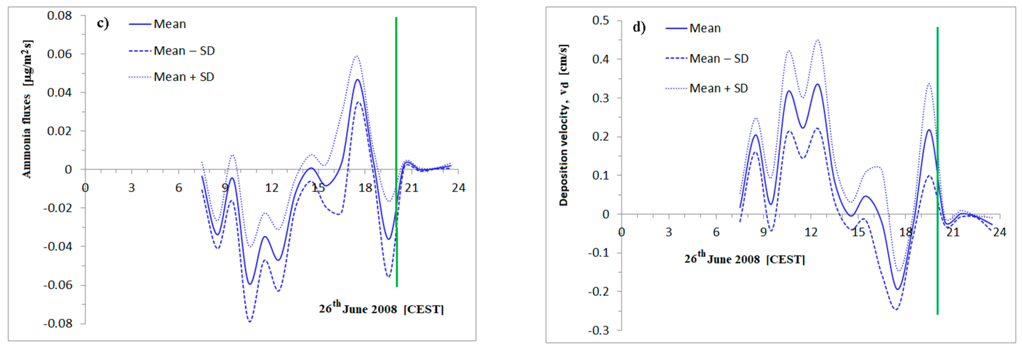
2.3. Ammonia Flux Estimation

Measurements provided an opportunity to estimate the ammonia logarithmic height gradients c ¯ l n z , flux F N H 3 and the traditional form of deposition velocity v d , giving their uncertainties. Hourly averaged and 5-min interpolated profiles with third-order polynomials were also analysed. Hourly concentration profiles were not strongly monotonous in the majority of the cases; therefore, we estimated the mean logarithmic concentration gradient on the 0.1–1.5 m layer. For each sublayer:
c ¯ l n z c ¯ l n z = c ¯ z 2 c ¯ z 1 l n z 2 l n z 1 ,
z r e f = z 1 · z 2 is the reference height. Here z 1 < z 2 is the height of the given levels and c ¯ z 1 ,   c ¯ z 2 are the mean concentrations for a time period. Five different approaches were used:
(i)
the mean gradient from 6 different sublayers based on 4 measurement levels
c ¯ l n z 1 = 1 6 i = 1 6 c ¯ z i c ¯ z j l n z i l n z j ,
where i = 2 ,   3 ,   4 ;   j = 1 ,   2 ,   3 and z i > z j (i > j ) .
The measurement levels were 0.1 m, 0.5 m, 1.0 m and 1.5 m,
(ii)
the median of logarithmic gradients for the 6 sublayers are presented below
c ¯ l n z 2 = M e d i a n c ¯ z i c ¯ z j l n z i l n z j ,
(iii)
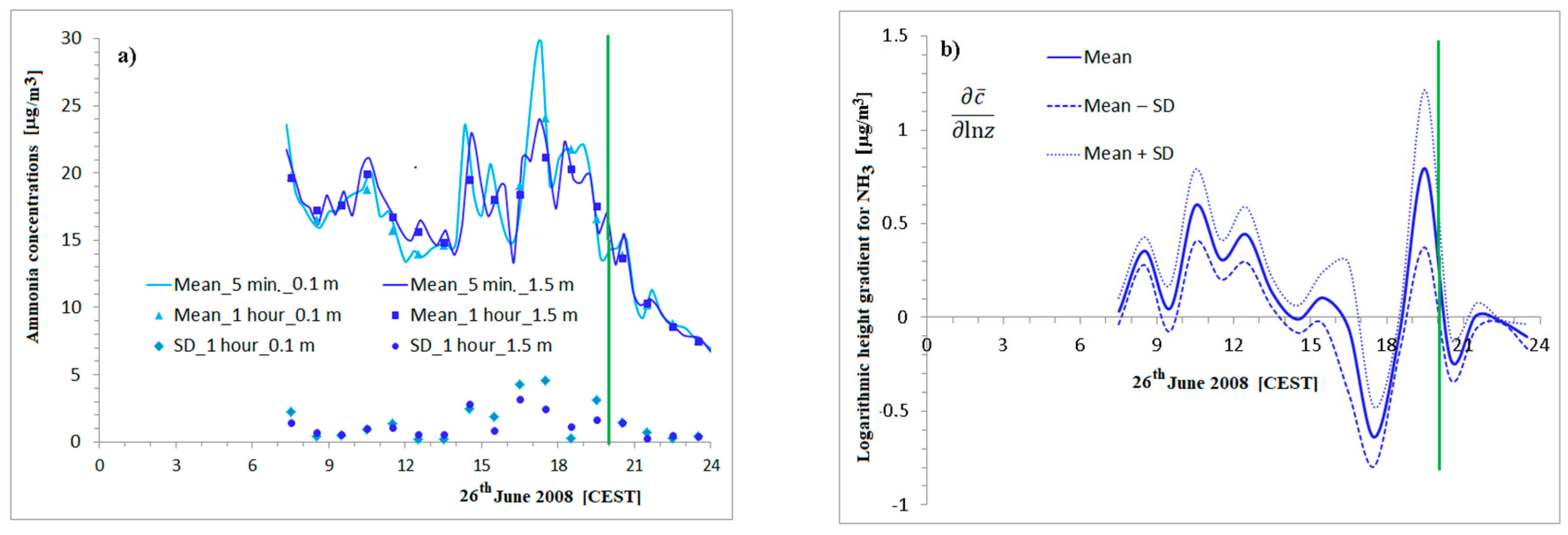
the logarithmic gradient for the two furthest top (1.5 m) and bottom (0.1 m) levels was also considered separately. Here, we expected the biggest differences, and thus the smallest uncertainty (the biggest differences give the least uncertainty)
c ¯ l n z 3 = c ¯ z 4 c ¯ z 1 l n z 4 l n z 1 ,
(iv)
the gradient calculated from the mean of the two lower and the two upper levels.
The reference heights are the geometric averages of each of the two levels
c ¯ l n z 4 = c ¯ z 4 + c ¯ z 3 c ¯ z 2 + c ¯ z 1 l n z 4 + l n z 3 l n z 2 + l n z 1 ,
(v)
the calculating the hourly gradient as the slope of a linear profile, c ¯ ^ z is estimated by the curve fitting
c ¯ ^ z = a · l n z + b ,
where a and b are fitted parameters for the logarithmic profile approximation using the least squares method
c ¯ l n z 5 = a .
The mean and standard deviation of the 5 logarithmic gradients were calculated for each hour
c ¯ l n z M e a n = 1 5 i = 1 5 c ¯ l n z i .
The next step is to determine the friction velocity ( u * ). Logarithmic profile approximation was used due to limited fetch and local advection and near the surface ( z 1 = 1.0   m and z 2 = 3.3   m ) the wind gradient measurement [22] was
u * = κ · u ¯ z 2 u ¯ z 1 l n z 2 l n z 1 ,
where κ = 0.4 is the von Karman constant. This meets the conditions of the measurement and is suitable for the first approximation [22].
More complex calculations for the friction velocity were also performed based on the Monin–Obukhov similarity theory using the universal functions of Dyer [27,28]. Due to the limited fetch and local advection effect, the average Bowen ratio of daytime hours (0.78) and measured available energy (net radiation–heat flux into the soil [29]) were used to estimate the sensible and latent heat fluxes for each 10-min time interval. The procedure that is more complex and has several uncertainties did not give any other result. An average 18% difference was found between the friction velocity calculated with the Monin–Obukhov similarity theory and with the logarithmic profile approximation. The u * calculated using the logarithmic approximation was usually the larger. Of course, when we implemented the stability function for the calculation form of the eddy diffusivity coefficient, it also changed shape [21,22].
The hourly averages of the friction velocity are calculated from the square root of the hourly average of the momentum fluxes. Knowing the mean estimated NH3 gradient c ¯ l n z M e a n and the friction velocity ( u * ) , taking advantage of neutral stratification near the surface, the ammonia flux was calculated as
F N H 3 = K N H 3 c ¯ z κ · u * · c ¯ l n z M e a n ,
where K N H 3 is the eddy diffusivity coefficient with the assumption of indifferent stratification, which is equal to the eddy diffusivity coefficient with sensible heat flux.
By knowing the ammonia flux, it is possible to estimate the traditional deposition velocity ( v d ) , which is calculated from its conventional definition as a ratio of vertical flux of ammonia to the mean concentration at a reference height in our case at 1.5 m above the surface [30]
v d = F N H 3 / c ¯   ( 1.5   m ) .
In practice, the deposition velocity was modelled through different types of resistances when the compensation points concentrations of different types of surfaces are known (leaves, bare soil, wet surfaces, etc.) [3,30]. The dry deposition flux ( F N H 3 ) was calculated in a widely used air pollution model (AERMOD), which uses the product of the concentration ( c ¯ ) and a deposition velocity ( v d ) calculated at a reference height [30].
The internal boundary layer height was established based on [22,31].

3. Results

Ammonia concentrations, the air temperature, relative humidity, wind speed and direction depending on time are shown in Figure 1a–e.
The highest hourly concentration of ammonia in the atmosphere was at a height of 0.5 m (24.09 ± 3.29 μg NH3/m3) between 16:00 and 17:00, when cows were grazing—as shown in Figure 1a. At the heights of 1.0 m and 1.5 m above the ground, the hourly mean gas concentrations between 16:00 and 17:00 were 23.21 ± 1.53 and 22.00 ± 1.75 μg NH3/m3, respectively, and the lowest was at the height of 0.1 m (20.69 ± 5.70 μg NH3/m3). The lowest ammonia content in the air was recorded between 23:00 and 24:00 at all heights above the ground and the smallest amount of this gas was 7.30 ± 0.40 μg NH3/m3 at a height of 1.5 m above the ground. Between 17:00 and 18:00 and at night—between 22:00 and 23:00—the ammonia concentration decreased with the increasing height above the ground. In the morning—between 8:00 and 9:00 and between 10:00 and 11:00—the concentration of this gas was high and increased with the increasing height above the ground—as shown in Figure 1a. In the case of increasing the concentration with the height, ammonia deposition occurs, which is typical near the cattle farm. The surface is a NH3 sink. The maximum concentration of gas (23.27 ± 5.70 μg NH3/m3) near the surface (0.1 m) was measured between 17:00 and 18:00 and it was the source of ammonia (the upward flux) from the farm—as shown in Figure 1a.
The daily average concentration of ammonia from all heights was 16.18 ± 0.63 μg NH3/m3 and its amount did not significantly depend on the height above the ground surface.
The highest air relative humidity (87.3 ± 1.3%), as the average of these two heights (0.8 and 3.2 m) above the ground, was between 23:00 and 24:00 CEST—as shown in Figure 1b. At a height of 0.8 m above the soil surface it was higher (89.9 ± 0.5%) than at a higher height (3.2 m), where the air relative humidity was 84.6 ± 2.1%. Dew formation began at 22:00 on the surface based on the leaf wetness sensor. The lowest air relative humidity was recorded between 16:00 and 17:00 and at a height of 0.8 m the relative humidity was 30.4 ± 0.4%, but at 3.2 m above the ground level it was 30.1 ± 0.5%. The relative humidity increased with the increasing height only in the morning from 7:00 to 12:00 and then decreased throughout the day—from after 12:00 until night—as shown in Figure 1 b. It is a typically unstable stratification with daytime evapotranspiration. The estimated maximum latent heat flux was 270 W/m2.
On 26 June 2008, the highest air temperature was recorded between 16:00 and 17:00 CEST (the average of the two heights was 25.1 ± 0.2 °C) and the lowest (24.7 ± 0.1 °C) was recorded at a height of 3.2 m, but the highest (25.5 ± 0.2 °C) was recorded at the height of 0.8 m—as shown in Figure 1c. The lowest temperature was recorded at night between 23:00 and 24:00 and the mean of the two heights was 12.4 ± 0.6 °C. At this time, the air temperature was higher (13.0 ± 0.6 °C) at a height of 3.2 m than at a height of 0.8 m (11.9 ± 0.5 °C). From 7:00 to 20:00, the air temperature decreased and from after 20:00 to approximately 24:00—it increased with the increasing height above the soil surface—as shown in Figure 1c.
The wind speed increased with the height above the ground from morning to night and was the highest between 11:00 and 12:00 at all heights (the average of the two heights was 3.6 ± 0.1 m/s), and at a height of 3.3 m its value was the highest (4.1 ± 0.1 m/s), while it was slightly lower at 1.0 m (3.2 ± 0.1 m/s)—as shown in Figure 1d. No wind was observed between 20:00 and 21:00 and between 23:00 and 24:00 at a height of 1.0 m above the ground and between 21:00 and 22:00 at a height of 3.3 m above the ground—as shown in Figure 1d. The start-up value of both wind sensors was approximately 0.3 m/s.
From 7:00 to 20:00, the wind direction expressed in degrees had the highest values of about 300 degrees, and between 19:00 and 20:00 it reached its maximum value (302°) when the west–northwest (WNW) direction of wind prevailed, while it reached its lowest value between 21:00 and 22:00 (150°) when the south–southeast (SSE) wind direction dominated—as shown in Figure 1e). The effect of the forest floor can be seen in large wind direction fluctuations from after 21:00 to 24:00 CEST as a result of the change in main wind direction—as shown in Figure 1e).
Independent of the height at which the air temperature, relative air humidity, wind speed and direction were measured, the ammonia concentration was always the lowest at height above the ground level (1.5 m) and amounted to 7.30 ± 0.4 μg NH3/m3 between 23:00 and 24:00 (at night) and the highest (24.09 ± 3.29 μg NH3/m3) at a height of 0.5 m between 16:00 and 17:00—as shown in Figure 1a–e). The highest average from four heights in terms of hourly gas concentration in the atmosphere was 22.49 ± 2.92 μg NH3/m3 between 16:00 and 17:00 and the lowest was 7.38 ± 0.15 μg NH3/m3 of air between 23:00 and 24:00—as shown in Figure 1a.
The average daily concentrations of ammonia in the air were as follows: 16.21 ± 0.88, 16.14 ± 0.44, 16.42 ± 0.59 and 15.99 ± 0.77 μg NH3/m3 at heights of 0.1, 0.5, 1.0 and 1.5 m above the ground, respectively. There was a non-strong monotonous profile. The daily concentration of ammonia in the atmosphere was the highest at 1.0 m, while the lowest was measured at 1.5 m above the ground. At heights of 0.8 and 3.2 m, the average daily air relative humidities were similar at 53.8 ± 0.1% and 51.7 ± 0.3%, respectively, and the air temperatures were 21.3 ± 0.1 °C and 21.2 ± 0.2 °C, respectively (which were practically the same), with the increasing height above the ground, while the mean daily relative humidity and the air temperature slightly decreased.
The mean daily wind speeds at heights of 1.0 and 3.3 m were 1.8 ± 0.1 and 2.3 ± 0.1 m/s, respectively, and the values increased with increasing height above the ground surface. The average daily value of the wind direction was measured only at 3.3 m above the ground and was 263 ± 10 degrees.
Figure 2 shows the increasing average values of the air’s relative humidity and temperature, as well as wind speed from the two heights tested, the mean concentration of ammonia in the air at different heights and the mean concentration of this gas from four heights.
The concentration of ammonia decreased with an increase in the average of the two heights (0.8 and 3.2 m above the ground) of the air’s relative humidity and was the highest at the height of 0.5 m of the tested gas (24.09 ± 3.29 μg NH3/m3) at the average relative air humidity of 30.2 ± 0.2% while it was lowest (7.30 ± 0.40 μg NH3/m3) at the height of 1.5 m, when the mean relative humidity of the air from the two heights was 87.2 ± 3.7%—as shown in Figure 2a.
The ammonia concentration increased with an increase in the average of the two heights (0.8 and 3.2 m above the ground), which affected the air temperature, and was the highest at the height of 0.5 m (24.09 ± 3.29 μg NH3/m3) at a mean air temperature of 25.1 ± 0.6 °C, while it was the lowest (7.30 ± 0.40 μg NH3/m3) at a height of 1.5 m, when the average of the two heights for the air’s temperature was 12.4 ± 0.8 °C—as shown in Figure 2b.
The ammonia concentration increased with the increasing wind speed. It was the highest at the height of 0.5 m and amounted to 24.09 ± 3.29 μg NH3/m3, while the average wind speed from the heights of 1.0 and 3.3 m was 2.3 ± 0.4 m/s and then decreased with further wind speeds—as shown in Figure 2c. The minimum concentration of gas (7.30 ± 0.40 μg NH3/m3) was recorded at a height of 1.5 m above the ground, when the average of the two heights of the wind speed was 0.05 ± 0.07 m/s—as shown in Figure 2c. Similar trends were observed when the concentration of ammonia was measured separately regarding its dependence on the air’s relative humidity, temperature and wind speed at each height above the ground.
The influence of wind direction on the concentration of ammonia in the air is presented in Figure 3.
With the increase in the value of the wind direction measured only at the height of 3.3 m, the ammonia concentration in the air increased, and its concentration was the highest at the height of 0.5 m (24.09 ± 3.29 μg NH3/m3), when the wind direction was 274 ± 11° and not its maximum value, as shown in Figure 3. The highest concentration of ammonia was recorded between 16:00 and 17:00, when cows were grazing outside and the west wind (W) was blowing from the farm with the animals towards the meteorological station and the photoacoustic instrument. The highest value for the west–northwest (WNW) direction of the wind (302 ± 6.0°) was recorded between 19:00 and 20:00, when the highest amount of ammonia was measured at a height of 1.0 m above the ground (16.54 ± 3.29 μg NH3/m3). The lowest ammonia content in the atmosphere was noted at 1.5 m above the ground (7.30 ± 0.40 μg NH3/m3) between 23:00 and 24:00, when the wind direction was 210 ± 109° south–southwest (SSW). The lowest value for wind direction (150 ± 123°) was between 21:00 and 22:00, when the lowest concentration of ammonia (9.59 ± 0.69 μg NH3/m3) was also measured at the height of 0.5 m. At this time it was a south–southeast (SSE) wind direction, as shown in Figure 3.
In this study, 5-min interpolated concentrations from 12:00 to 21:00 CEST are calculated using cubic polynomials and are illustrated, as shown in Figure 4, we experienced intense plumes. The plumes are visible near the surface (maximum values at 0.1 m in periods from 14:15 to 14:25 and from 16:45 to 17:30) and in the upper two levels (0.5 and 1.0 m) in the time period from 18:50 to 19:25.
Measurements provided limited fetch conditions. The estimation of internal boundary layer height ( δ h )
δ h = 0.3 · x
was calculated. In the equation, x   [m] is the distance of the measuring site from the forest belt or the barn. The cases of 20, 30 and 100 m limited fetch ( δ h ) achieved values of 1.3, 1.6 and 3.0 m, respectively. The height of 1.5 m for the ammonia concentration profile measurement is suitable, but the 3.2–3.3 m levels for the upper wind, air temperature and relative humidity measurements are too high when the air comes from the direction of the forest belt. Measurements after 20:00 CEST provided turbulent fluxes around zero due to the stable stratification and low wind speed—as shown in Figure 1c,d.
The wind profile is more important when calculating the turbulent diffusion coefficient for a sensible heat due to the near-surface stratification close to the logarithmic.
In the following section, the main steps of NH3 flux calculation are presented. In the end, we present the flux calculation results based on the assumption of neutral profile approximation—Section 2.3. First, we investigated the concentration–time series from 0.1 m to 1.5 m to interpret gradients—as shown in Figure 5a. The 5-min and hourly mean concentrations, as well as the standard deviations calculated from 5-min data, are presented.
The difference in mean hourly concentrations at 0.1–1.5 m levels determined using polynomial (the 5-min interpolated time resolution) and original (3 measurements from each hour) averaging (see Section 2.1) was 0.18 μg NH3/m3, while the difference in the mean standard deviations of the hourly concentrations determined using polynomial and original averaging was 1.00 μg NH3/m3. The reason for the suitable differences between the two standard deviations is the difference in the description of the plumes—as compared in Figure 1a, Figure 4 and Figure 5a. The maximum measured value of the 5-min average concentration was 29.77 μg NH3/m3 (from 17:15 to 17:20) at the height of 0.5 m. Concentrations at 1.5 m are greater than those at 0.1 m in most cases. The deposition (turbulent fluxes into the surface with the negative sign) is expected—as shown in Figure 5c. The impact of plumes is clearly visible in the higher concentrations at the height of 0.1 m and in the shift in concentration maximums towards higher levels. In several cases, the peaks on the 1.5 m level are detected later. There are high standard deviations at this time. High concentrations on the bottom of the layer (0.1 m) are reflected in the positive values of gradients estimated using five different methods during the late afternoon (from 16:00 to 18:00 CEST).
The mean logarithmic concentration gradients are presented in Figure 5b. The daily variations in ammonia fluxes with ± standard deviations are shown in Figure 5c. The hourly means of the absolute values of concentration gradients are also presented. M e a n c ¯ l n z i and its standard deviation S D c ¯ l n z i were also determined. The ratio of the mean hourly standard deviation to the mean hourly absolute gradient is
M e a n c ¯ l n z i / S D c ¯ l n z i = 0.154 0.194 = 0.79 ,
which suggests the high uncertainty of the gradient calculation. This is an outlier among the profiles, the majority of which are non-monotonous. The uncertainty proceeds as follows: the ammonia flux curves like the course of the gradients, presenting the uncertainties. The turbulent diffusion coefficient with the assumption of neutral stratification is a good approximation that follows the wind speed variation. The effect of the late afternoon ammonia plume (the source effect) is comparable with early afternoon negative ammonia fluxes on the surface (a sink), and this is also presented. The ammonia surface flux is bidirectional, as we can see in Figure 5c; that is, the net flux can be either upward or downward.
The traditional deposition velocity of ammonia is presented in Figure 5d. The maximum value in the early afternoon ( v d ) M a x = 0.33 ± 0.11   c m / s was detected. In the late afternoon (from 16:00 to 18:00 CEST), when the maximum ammonia concentrations were measured at the bottom, the traditional deposition velocities are negative, for example:
v d 18 : 00   C E S T = 0.19 ± 0.05   c m / s .

4. Discussion

During our research, the concentration of ammonia increased with the increasing air temperature. The same relationship was also obtained by Sutton et al. [32], Mkhabela et al. [33], Teng et al. [34] and Qu et al. [35]. The gas concentration was higher during the day than at night. Similar results were also achieved by Huber and Kreutzer [36], Sutton et al. [32] and Walker et al. [37]. In this case, the concentration of ammonia closer to the ground was higher than at higher heights. This is confirmed by Sutton et al. [32] and Denmead et al. [38]. When it was warmer (in the afternoon), higher gas concentrations were recorded than when it was cooler (at night). Additionally, Sutton et al. [32] noted the same trend.
The gas concentration depends on the wind direction, which is also confirmed by Teng et al. [34] and Qu et al. [35]. In the current work, the highest ammonia concentration was when the west wind direction—W (274 ± 11°)—was blowing from the farm with 430 cows. The lowest ammonia content in the atmosphere was recorded during the south–southwest wind—SSW (210 ± 109°)—which occurred at night. The 5-min interpolated profile dataset can be used to analyse ammonia plumes caused by animal husbandry. This causes non-monotonous surface NH3 profiles, which are further modified by limited fetch and local advection.
The results of the present work indicate that the gas concentration does not significantly depend on the wind speed, which was also confirmed by Huber and Kreutzer [36]. At wind speeds of 2.1 ± 0.3 m/s at 1.0 m and 2.6 ± 0.4 m/s at 3.3 m, ammonia concentrations were the highest, but when wind speeds exceeded 3.0 m/s, lower gas concentrations were recorded. At very low wind speeds (≤0.1 m/s) at 1.0 and 3.3 m above the ground, respectively the gas concentration was the lowest (7.30 ± 0.40 μg/m3). We know the typical daily variations in wind speed and direction, which achieve the lowest values after sunset and the highest values in the daytime. With the increasing wind speed, the emission of ammonia from dairy barns increased [39]; however, too-high wind velocities (above 5–6 m/s) reduced the ammonia concentration by more than 50% [32]. Therefore, this is a case study that emphasises the importance of local effects.
In our experiment, the highest concentration of ammonia (24.09 ± 3.29 μg/m3) was recorded at the lowest relative humidity values for the air (30.4 ± 0.4% and 30.1 ± 0.5%), and the lowest values (7.30 ± 0.40 μg/m3) at 89.9 ± 0.5% and 84.6 ± 2.1% for the air’s relative humidities were recorded at heights of 0.8 and 3.2 m above the ground, respectively, while the gas concentration decreased with an increase in the air’s relative humidity. The same correlation was confirmed by Qu et al. [35] and Huber and Kreutzer [36]; however, for the latter authors, maximal concentrations of ammonia were noted in the range from 40% to 50% of air’s relative humidity, while the lowest concentration values were achieved when the air’s relative humidity had higher values (between 90 and 95%).
Our research was performed in the summer of 2008 in Rogaczewo Wielkie, Poland, approximately 100 m from a cattle farm. The mean hourly concentrations of ammonia recorded with the Nitrolux 1000 equipment ranged from 7.30 ± 0.40 μg NH3/m3 around midnight—between 23:00 and 24:00, when the animals were locked in a barn and the air temperature was the lowest. The highest hourly ammonia concentration (24.09 ± 3.29 μg NH3/m3) was during the day between 16:00 and 17:00 h, when 430 cows were outside the cattle farm and the west wind direction was blowing from the cowshed and the mean air temperature was 25.5 ± 0.2 °C at the height of 0.8 m. It was the highest hourly temperature of the day. The main reason for high ammonia levels was the presence of animals. The mean daily ammonia concentration in the air from all heights was 16.18 ± 0.63 μg NH3/m3. Acceptable hourly and daily ammonia contents in the air are 3300 and 270 μg NH3/m3 according to Van der Eerden et al. [39]; therefore, the air was clean. The lowest concentration of ammonia was at night, when there was an absence of wind and air temperatures were at their lowest values (11.9 ± 0.5 °C) at the height of 0.8 m above the ground. Additionally, Huber and Kreutz [36] obtained the same environmental results related to ammonia concentrations in the air.
We analysed the uncertainty resulting from the estimation of near-surface ammonia gradient based on the profile measurements. The hourly mean fluxes and traditional deposition velocities were calculated. The maximum flux (deposition) formed in the early afternoon when its value was 58.9 ± 19.6 · 10 3   μg/m2·s. The relative standard deviation was high (33%). Further uncertainty comes from the estimation of the friction velocity (the choice of the methodology, the estimation of the mean Bowen ratio, etc.). The maximum value of the traditional deposition velocity was ( v d ) M a x = 0.33 ± 0.11   c m / s in the early afternoon, which fits the previous calculation results [40]. Due to the proximity of the livestock farm, a negative deposition velocity of up to 0.2   c m / s was detected over several hours.
In our work, the structure of flux divergence can be inferred from the concentration profiles as the place of minimum and maximum concentrations inside the 0.1–1.5 m layer. This does not allow the direct application the Monin–Obukhov similarity theory for the calculation of flux [27,28]. The turbulent flux and its uncertainty are quantified through the mean concentration gradient estimation. This is the reason we apply the near-surface 0.1–1.5 m layer for the logarithmic (neutral) profile assumption based on Section 2.2.
Our research shows that the presence of cows outside the farm has the greatest influence on the content of ammonia in the air, followed by the time of day, air temperature and wind direction; then, the wind speed and height above the ground surface and finally the air relative humidity. These conclusions confirm our previous hypotheses. Understanding the factors affecting the concentration of ammonia in the atmosphere will allow us to control its amount in nature in the future, e.g., by using manure at lower air temperatures and at higher air relative humidity values.

5. Conclusions

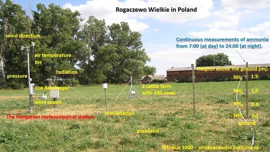
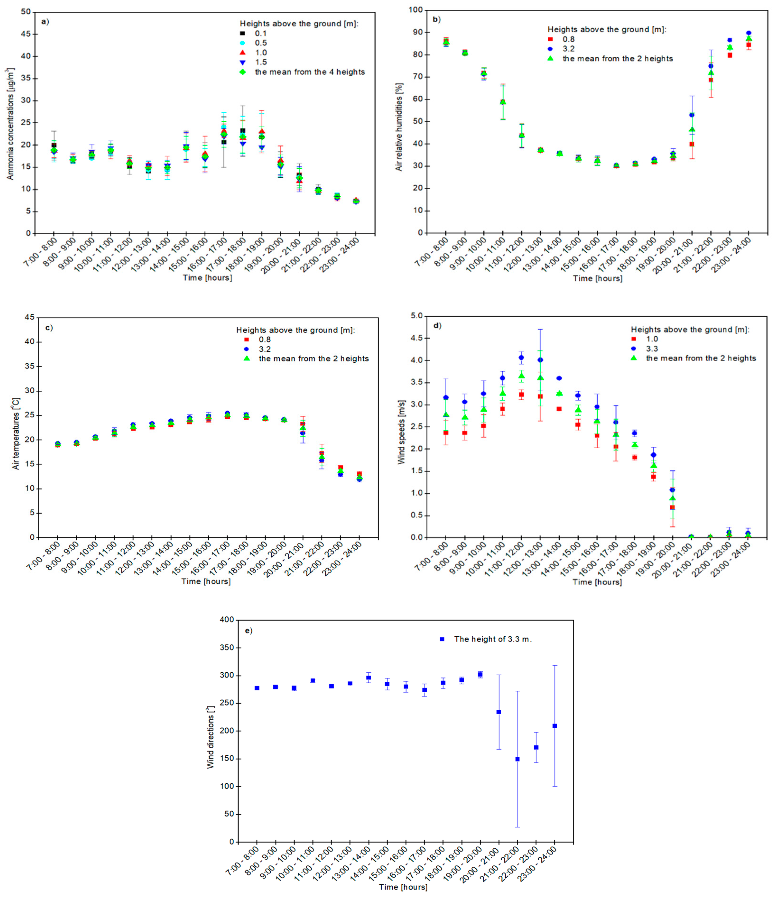
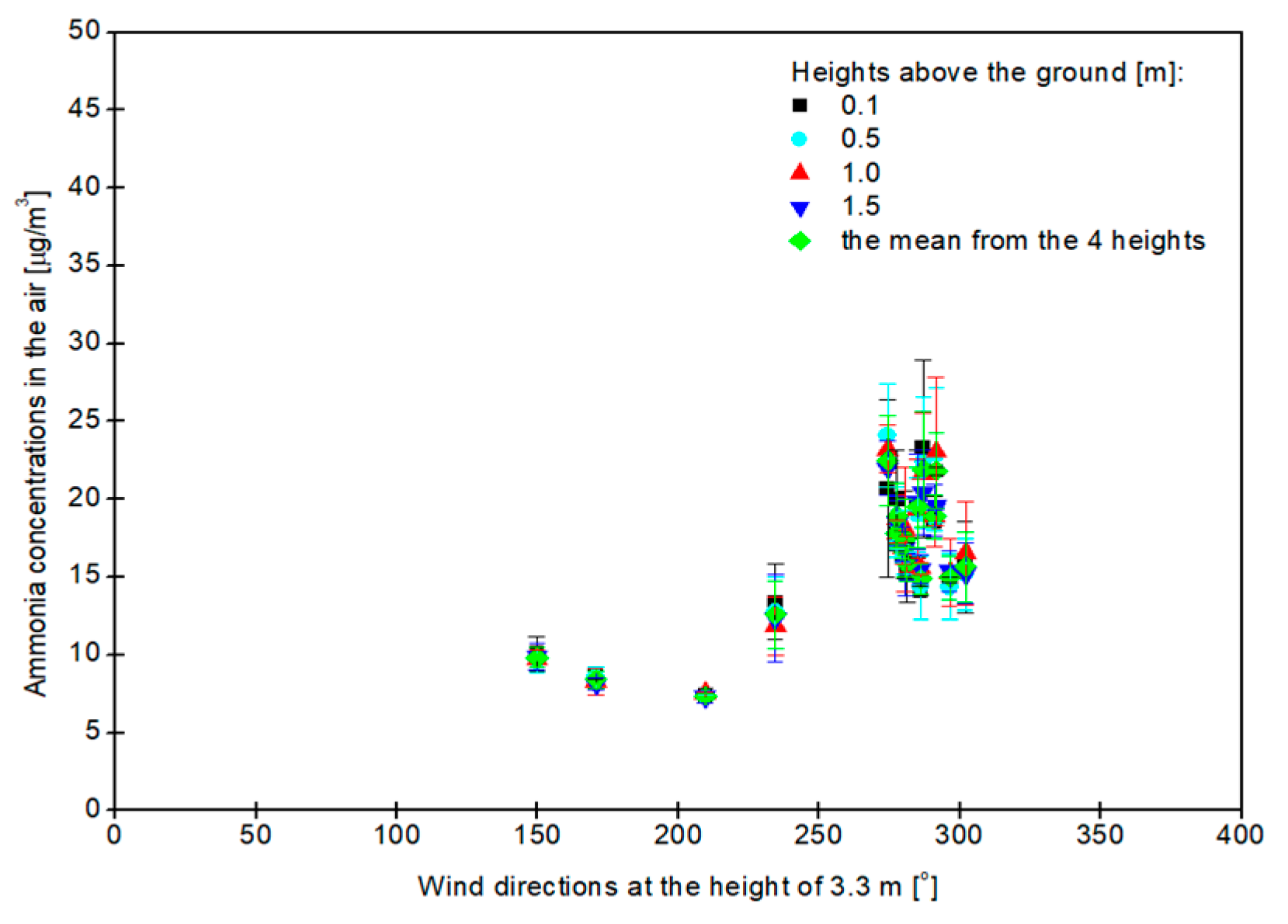
  • The ammonia concentration depended most on the presence of 430 grazing cows on the farm in Rogaczewo Wielkie in Poland (the latitude 52°01′60.00″ N and a longitude 16°49′59.99″ E) and time of day (the highest concentration was in the late afternoon and the lowest at night). The gas content in the atmosphere coincided with the dynamics of changes in the wind direction over time, and was the highest when the wind was blowing westerly from the farm’s direction. We draw attention to the importance of quantifying local effects and special micrometeorological measurements.
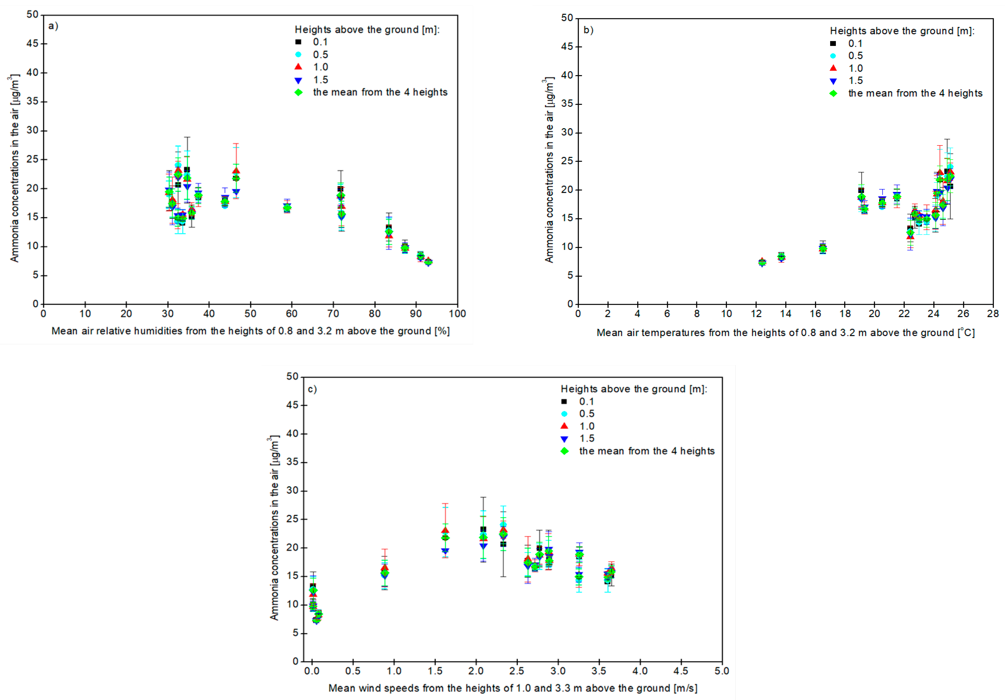
  • The ammonia concentration decreased with increases in the relative air humidity and increased with the increasing air temperature. The amount of gas in the air depended slightly less on the air temperature and relative air humidity.
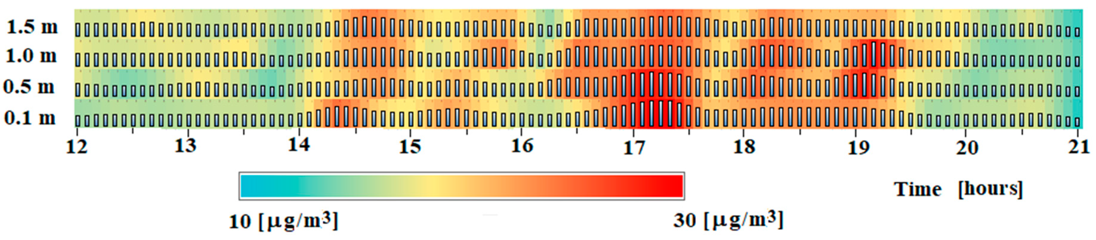
  • The wind speed and height above the ground did not significantly affect the concentration of ammonia in the air on the 0.1–1.5 m layer. The hourly concentration of this gas in the atmosphere was the highest at the height of 0.5 m above the ground when the mean wind speed from the heights of 1.0 and 3.3 m above the ground achieved 2.3 m/s and above this value of the wind speed the concentration of ammonia decreased, but the highest daily amount of this gas was at a height of 1.0 m above the ground.
  • Based on the profile measurements, the ammonia gradient characteristics of the 0.1–1.5 m layer were determined. It is rare to experience strongly monotonous profiles.
  • The hourly and daily concentrations of ammonia approximately 100 m from the farm with cows did not exceed critical values; therefore, no air pollution in terms of this gas was found.

Author Contributions

Conceptualisation, B.K. and T.W.; Methodology, B.K. and T.W.; Software, B.K. and T.W.; Validation, B.K. and T.W.; Formal Analysis, B.K. and T.W.; Investigation, B.K. and T.W.; Resources, B.K. and T.W.; Data Curation, B.K. and T.W.; Writing—Original Draft Preparation, B.K. and T.W.; Writing—Review and Editing, B.K.; Visualisation, B.K. and T.W.; Supervision, B.K. and T.W.; Project Administration, B.K. and T.W.; Funding Acquisition, B.K. and T.W. All authors have read and agreed to the published version of the manuscript.

Funding

The study was financed by the Institute for Agricultural and Forest Environment, Polish Academy of Sciences in Poznań, Poland, with NitroEurope Integrated Project No. 17841 (2006–2011) entitled “The nitrogen cycle and its influence on the European greenhouse gas balance”, which was a part of the EU’s Sixth Framework Programme for Research and Technological Development. The final data analysis was partly supported by the National Research, Development and Innovation Office Grant K138176 and the FAIR Network of micrometeorological measurements COST Action (CA20108).

Institutional Review Board Statement

Not applicable.

Informed Consent Statement

Not applicable.

Data Availability Statement

All measured data are available from the authors upon request.

Acknowledgments

The authors of this paper would like to thank the employees of the Institute of Agricultural and Forest Environment, Polish Academy of Sciences, Poznań, Poland: Andrzej Kędziora—for initiating Polish—Hungarian scientific cooperation under the NitroEurope project, Jakub Wasilewski—for cooperation in carrying out measurements with Beata Kułek, who organised the international field campaign in Rogaczewo Wielkie (Poland) in June 2008 and activated the NitroluxTM Ammonia Analyser Model 1000 for measurements and the Hungarian participants of the campaign in particular: Arpad Bordás and András Gyöngyösi Zénó from the Eötvös Loránd University, Attila Eredics from the Sopron University and Laszlo Horvath from the Research Group ELKH-SZTE, Szeged, Hungary—for photoacoustic monitoring of environmental processes, recording the meteorological data and for their cooperation during and after the field campaign.

Conflicts of Interest

The authors declare no conflict of interest. The sponsors had no role in the design, execution, interpretation or writing of the research article.

References

  1. Kachniarz, M. Latrines, SNAP code 091007. In Joint EMEP/CORINAIR Atmospheric Emission Inventory Guidebook; McInnes, G., Ed.; EEA: Copenhagen, Denmark, 1996. [Google Scholar]
  2. Van der Hoek, K.W. Estimating ammonia emission factors in Europe: Summary of the work of the UNECE ammonia expert panel. Atmos. Environ. 1998, 32, 315–316. [Google Scholar] [CrossRef]
  3. Sutton, M.A.; Howard, C.M.; Erisman, J.W.; Billen, G.; Bleeker, A.; Grennfelt, P.; Van Grinsven, H.; Grizzetti, B. The European Nitrogen Assessment: Sources, Effects and Policy Perspectives; Cambridge University Press: Cambridge, UK, 2011; 664p, ISBN 9781107006126. [Google Scholar]
  4. Sommer, S.G.; Webb, J.; Hutchings, N.D. New Emission Factors for Calculation of Ammonia Volatilization from European Livestock Manure Management Systems. Front. Sustain. Food Syst. 2019, 3, 101. [Google Scholar] [CrossRef]
  5. Theobald, M.R.; Dragosits, U.; Place, C.J.; Smith, J.U.; Sozanska, M.; Brown, L.; Scholefield, D.; Del Prado, A.; Webb, J.; Whitehead, P.G.; et al. Modelling nitrogen fluxes at the landscape scale. Water, Air, and Soil Pollut. Focus 2004, 4, 135–142. [Google Scholar] [CrossRef]
  6. Fowler, D.; Pitcairn, C.E.R.; Sutton, M.A.; Flechard, C.; Loubt, B.; Coyle, M.; Munro, R.C. The mass budget of atmospheric ammonia in woodland within 1 km of livestock buildings. Environ. Pollut. 1998, 102, 343–348. [Google Scholar] [CrossRef]
  7. Liu, L.; Xu, W.; Lu, X.; Zhong, B.; Guo, Y.; Lu, X.; Zhao, Y.; Heg, W.; Wangh, S.; Zhangg, X.; et al. Exploring global changes in agricultural ammonia emissions and their contribution to nitrogen deposition since 1980. Proc. Natl. Acad. Sci. USA 2022, 119, e2121998119. [Google Scholar] [CrossRef] [PubMed]
  8. Erisman, J.W.; Vermeulen, A.; Hensen, A.; Fléchard, C.; Dämmgen, U.; Fowler, D.; Sutton, M.; Grünhage, L.; Tuovinen, J.P. Monitoring and modelling of biosphere/atmosphere exchange of gases and aerosols in Europe. Environ. Pollut. 2005, 133, 403–413. [Google Scholar] [CrossRef] [PubMed]
  9. Mosquera, J.; Monteny, G.J.; Erisman, J.W. Overview and assessment of techniques to measure ammonia emissions from animal houses: The case of the Netherlands. Environ. Pollut. 2005, 135, 381–388. [Google Scholar] [CrossRef] [PubMed]
  10. Von Bobrutzki, K.; Müller, H.J.; Scherer, D. Factors affecting the ammonia content in the air surrounding a broiler farm. Biosyst. Eng. 2011, 108, 322–333. [Google Scholar] [CrossRef]
  11. Kunes, R.; Havelka, Z.; Olsan, P.; Smutny, L.; Filip, M.; Zoubek, T.; Bumbalek, R.; Petrovic, B.; Stehlik, R.; Bartos, P.A. Review: Comparison of Approaches to the Approval Process and Methodology for Estimation of Ammonia Emissions from Livestock Farms under IPPC. Atmosphere 2022, 13, 2006. [Google Scholar] [CrossRef]
  12. Warneck, P. Chemistry of the Natural Atmosphere (International Geophysics Series); Academic Press: San Diego, CA, USA, 1988; Volume 41, pp. 426–441. [Google Scholar] [CrossRef]
  13. Sutton, M.A.; Fowler, D.; Moncrieff, J.B.; Storeton-West, R.L. The exchange of atmospheric ammonia with vegetated surfaces. II: Fertilized vegetation. Quart. J. Roy. Meteor. Soc. 1993, 119, 1047–1070. [Google Scholar] [CrossRef]
  14. Galloway, J.N. Acid deposition: Perspectives in time and space. Water Air Soil Pollut. 1995, 85, 15–24. [Google Scholar] [CrossRef]
  15. National Science and Technology Council (U.S.), Air Quality Research Subcommittee. Atmospheric Ammonia: Sources and Fate. A Review of Ongoing Federal Research and Future Needs; United States, Office of Science and Technology Policy: Washington, DC, USA; Available online: https://digital.library.unt.edu/ark:/67531/metadc25995/ (accessed on 11 August 2023).
  16. Boero, A.; Mercier, A.; Mounaïm-Rousselle, C.; Valera-Medina, A.; Ramirez, A.D. Environmental assessment of road transport fueled by ammonia from a life cycle perspective. J. Clean. Prod. 2023, 390, 136–150. [Google Scholar] [CrossRef]
  17. Nitrogen Still a Major Threat to Ecosystems in Large Parts of Europe. 2023. Available online: https://unece.org/environment/news/nitrogen-still-major-threat-ecosystems-large-parts-europe (accessed on 11 August 2023).
  18. Horváth, L.; Fagerli, H.; Sutton, M.A. Long-Term Record (1981–2005) of Ammonia and Ammonium Concentrations at K-Puszta Hungary and the Effect of Sulphur Dioxide Emission Change on Measured and Modelled Concentrations. In Atmospheric Ammonia; Springer: Berlin/Heidelberg, Germany, 2009; pp. 181–185. [Google Scholar] [CrossRef]
  19. Trebs, I.; Junk, J.; Ammann, C. Immission and Dry Deposition. In Springer Handbook of Atmospheric Measurements; Chapter 54; Foken, T., Ed.; Springer: Cham, Switzerland, 2021; pp. 1445–1472. [Google Scholar] [CrossRef]
  20. Huszár, H.; Pogány, A.; Bozóki, Z.; Mohácsi, Á.; Horváth, L.; Szabó, G. Ammonia monitoring at ppb level using photoacoustic spectroscopy for environmental application. Sens. Actuators B Chem. 2008, 134, 1027–1033. [Google Scholar] [CrossRef]
  21. Arya, S.P. Introduction to Micrometeorology, 2nd ed.; Academic Press: San Diego, CA, USA, 2001; 415p, ISBN 0120593548. [Google Scholar]
  22. Foken, T. Micrometeorology, 2nd ed.; Springer: Berlin/Heidelberg, Germany, 2017; 362p. [Google Scholar] [CrossRef]
  23. Weidinger, T.; Pogany, A.; Janku, K.; Wasilewsky, J.; Mohacsi, A.; Bozoki, Z.; Gyongyosi, A.Z.; Istenes, Z.; Eredics, A.; Bordas, A. Micrometeorological and ammonia gradient measurements above agricultural fields in Turew (Poland). In Proceedings of the European Geosciences Union General Assembly 2009, Vienna, Austria, 19–24 April 2009; p. 8167. Available online: http://meetings.copernicus.org/egu2009 (accessed on 11 August 2023).
  24. Mauder, M.; Foken, T. Documentation and Instruction Manual of the Eddy-Covariance Software Package TK3 (Update); Universität Bayreuth: Bayreuth, Germany, 2015; 68p, ISSN 1614-8924. [Google Scholar]
  25. Pogány, A.; Weidinger, T.; Bozóki, Z.; Mohácsi, Á.; Bieńkowski, J.; Józefczyk, D.; Eredics, A.; Bordás, Á.; Gyöngyösi, A.Z.; Horváth, L.; et al. Application of a novel photoacoustic instrument for ammonia concentration and flux monitoring above agricultural landscape-results of a field measurement campaign in Choryń, Poland. Időjárás 2012, 116, 93–107. [Google Scholar]
  26. Pogány, A.; Mohácsi, S.K.; Jones, E.; Nemitz, A.; Varga, Z.; Bozóki, Z.; Galbács, T.; Weidinger, T.; Horváth, L.; Szabó, G. Evaluation of a diode laser based photoacoustic instrument combined with preconcentration sampling for measuring surface-atmosphere exchange of ammonia with the aerodynamic gradient method. Atmos. Environ. 2010, 44, 1490–1496. [Google Scholar] [CrossRef]
  27. Dyer, A.J.; Hicks, B.B. Flux-gradient relationships in the constant flux layer. Quart. J. Roy. Meteorol. Soc. 1970, 96, 715–721. [Google Scholar] [CrossRef]
  28. Dyer, A.J. A review of flux-profile-relationships. Boundary-Layer Meteorol. 1974, 7, 363–372. [Google Scholar] [CrossRef]
  29. Liebethal, C.; Foken, T. Evaluation of six parameterization approaches for the ground heat flux. Theor. Appl. Climatol. 2007, 88, 43–56. [Google Scholar] [CrossRef]
  30. Phillips, S.B.; Arya, S.P.; Aneja, V.P. Ammonia flux and dry deposition velocity from near-surface concentration gradient measurements over a grass surface in North Carolina. Atmos. Environ. 2004, 38, 3469–3480. [Google Scholar] [CrossRef]
  31. Raabe, A. On the relation between the drag coefficient and fetch above the sea in the case of off-shore wind in the near shore zone. Z. Meteorol. 1983, 33, 363–367. [Google Scholar]
  32. Sutton, M.A.; Nemitz, E.; Fowler, D.; Wyers, G.P.; Otjes, R.P.; Schjoerring, J.K.; Husted, S.; Nielsen, K.H.; San José, R.; Moreno, J.; et al. Fluxes of ammonia over oilseed rape: Overview of the EXAMINE experiment. Agric. For. Meteorol. 2000, 105, 327–349. [Google Scholar] [CrossRef]
  33. Mkhabela, M.S.; Gordon, R.; Burton, D.; Smith, E.; Madami, A. The impact of management practices and meteorological conditions on ammonia and nitrous oxide emissions following application of hog slurry to forage grass in Nova Scotia. Agr. Ecosyst. Environ. 2009, 130, 41–49. [Google Scholar] [CrossRef]
  34. Teng, X.; Hu, Q.; Zhang, L.; Qi, J.; Shi, J.; Xie, H.; Gao, H.; Yao, X. Identification of major sources of atmospheric NH3 in an urban environment in northern China during wintertime. Environ. Sci. Technol. 2017, 51, 6839–6848. [Google Scholar] [CrossRef]
  35. Qu, Q.; Groot, J.C.J.; Zhang, K.; Schulte, R.P.O. Effects of housing systems, measurement methods and environmental factors on estimating ammonia and methane emission rates in dairy barns: A meta-analysis. Biosyst. Eng. 2021, 205, 64–75. [Google Scholar] [CrossRef]
  36. Huber, C.; Kreutzer, K. Three years of continuous measurements of atmospheric ammonia concentrations over a forest stand at the Höglwald site in southern Bavaria. Plant Soil 2002, 240, 13–22. [Google Scholar] [CrossRef]
  37. Walker, J.T.; Robarge, W.P.; Wu, Y.; Meyers, T.P. Measurement of bi-directional ammonia fluxes over soybean using the modified Bowen-ratio technique. Agric. For. Meteorol. 2006, 138, 54–68. [Google Scholar] [CrossRef]
  38. Denmead, O.T.; Chen, D.; Griffith, D.W.T.; Loh, Z.M.; Bai, M.; Naylor, T. Emissions of the indirect greenhouse gases NH3 and NOx from Australian beef cattle feedlots. Aust. J. Exp. Agric. 2008, 48, 213–218. [Google Scholar] [CrossRef]
  39. Van der Eerden, L.J.; Dueck, T.A.; Berdowski, J.J.M.; Greven, H.; Van Dobben, H.F. Influence of NH3 and (NH4)2SO4 on heathland vegetation. Acta Bot. Neerl. 1991, 40, 281–296. [Google Scholar] [CrossRef]
  40. Schrader, F.; Bruemmer, C. Land Use Specific Ammonia Deposition Velocities: A Review of Recent Studies (2004–2013). Water Air. Soil. Pollut. 2014, 225, 2114. [Google Scholar] [CrossRef]
Figure 1. The effect of the time of day on the ammonia concentration (a), relative air humidity (b) and air temperature (c) as well as wind speed (d) and direction (e) on 26 June 2008 in Rogaczewo Wielkie in Poland (the 1-h time resolution, CEST time). Hourly NH3 concentration was calculated with an arithmetical average of the 3 measured values between the hours indicates in figures. The vertical line above the symbol means the standard deviation (SD).
Atmosphere 14 01703 g001
Figure 2. The effect of increasing the air relative humidity (a), air temperature (b) and wind speed (c) averaged from 2 tested heights on the content of ammonia measured at 4 heights in the air and on the mean concentration of this gas averaged from 4 heights.
Atmosphere 14 01703 g002
Figure 3. The effect of wind direction at 3.3 m above the soil surface on the concentration of ammonia in the atmosphere at 0.1, 0.5, 1.0 and 1.5 m above the ground. The mean gas concentration from the 4 tested heights is also shown.
Atmosphere 14 01703 g003
Figure 4. The plume detection based on 5-min ammonia profiles using a third-order polynomial approximation for interpolation at each layer in a period of formation of plumes from 12:00 to 21:00 CEST on 26 June 2008.
Atmosphere 14 01703 g004
Figure 5. The ammonia flux and deposition velocity calculation step by step. The ammonia concentration at 0.1 m and 1.5 m levels. 5-min and 1-h averages and hourly standard deviations—top-left, (a). A daily course of hourly logarithmic height gradients of NH3 and standard deviations based on 5 different calculation methods—top-right, (b); estimated fluxes with SD—bottom-left, (c); estimation of the traditional deposition velocity of ammonia with SD—bottom-right, (d). The wind speed at 3.3 m was smaller than 0.5 m/s from 21:00 CEST, ( u * ) M i n = 0.03   m / s . Green line: the border of the low wind speed (21:00 CEST).
Atmosphere 14 01703 g005aAtmosphere 14 01703 g005b
Disclaimer/Publisher’s Note: The statements, opinions and data contained in all publications are solely those of the individual author(s) and contributor(s) and not of MDPI and/or the editor(s). MDPI and/or the editor(s) disclaim responsibility for any injury to people or property resulting from any ideas, methods, instructions or products referred to in the content.

