Abstract
Monoterpenes significantly affect air quality and climate as they participate in tropospheric ozone formation, new particle formation (NPF), and growth through their oxidation products. Vegetation is responsible for most biogenic volatile organic compound (BVOC) emissions released into the atmosphere, yet the contribution of shrub and regional transport to the ambient monoterpene mixing ratios is not sufficiently documented. In this study, we present one-year systematic observations of monoterpenes in the Eastern Mediterranean at a remote coastal site, affected mainly by the typical phrygana vegetation found on the Island of Crete in Greece. A total of 345 air samples were collected in absorption tubes and analyzed by a GC-FID system during three intensive campaigns (in spring 2014, summer 2014, and spring 2015) in addition to the systematic collection of one diurnal cycle per week from October 2014 to April 2015. Limonene, α-pinene and 1,8-cineol have been detected. The mixing ratios of α-pinene during spring and summer show a cycle that is typical for biogenic compounds, with high levels during the night and early morning, followed by an abrupt decrease around midday, which results from the strong photochemical depletion of this compound. Limonene was the most abundant monoterpene, with average mixing ratios of 36.3 ± 66 ppt. The highest mixing ratios were observed during autumn and spring, with a maximum mixing ratio in the early afternoon. The spring and autumn maxima could be attributed to the seasonal behavior of vegetation growth at Finokalia. The green period starts in late autumn when phrygana vegetation grows because of the rainfall; the temperature is still high at this time, as Finokalia is located in the southeast part of Europe. Statistical analyses of the observations showed that limonene and α-pinene have different sources, and none of the studied monoterpenes is correlated with the anthropogenic sources. Finally, the seasonality of the new particle formation (NPF) events and monoterpene mixing ratios show similarities, with a maximum occurring in spring, indicating that monoterpenes may contribute to the production of new particles.
1. Introduction
Monoterpenes affect the oxidizing capacity of the atmosphere since they react rapidly with the main oxidants of the troposphere, namely hydroxyl (OH), nitrate (NO3) radicals and ozone (O3), and their oxidation contributes to tropospheric O3 formation when sufficient amounts of nitrogen oxides are available [1,2]. Moreover, their low-volatility oxidation products are involved in new particle formation (NPF) and growth processes [3,4,5]. O3 is a greenhouse gas [6] and is phytotoxic [7], thus affecting human health [8]. Furthermore, NPF and growth are found to increase cloud condensation nuclei by 29 to 77% in the East Mediterranean [9], having significant climate effects through their interactions with light and clouds, and impacting human health. Air pollution from fine aerosols is estimated to have led to 238,000 premature deaths in the European Union in 2020 [10]. In order to evaluate the contribution of monoterpenes to these effects, the determination of their atmospheric mixing ratios is needed.
Atmospheric monoterpenes have both natural and anthropogenic sources. The emissions of atmospheric volatile organic compounds (VOCs) by vegetation, which is their largest natural source [11], are ecologically important, as vegetation uses VOCs to protect itself against high temperatures [12,13], high irradiance [14] and oxidative stress [15]. Furthermore, VOCs act as plant-to-plant [16], plant-to-pollinator [17] and plant-to-herbivore communication signals [15]. Even though the main sources of monoterpenes on a global scale are natural, anthropogenic emissions can be the most important sources in urban areas. They are related to vehicular exhausts [18], heating activities [19], volatile chemical products use (e.g., cleaning products) [20], tree combustion [21] and industrial activities [22].
Monoterpenes have been measured with various offline and online analytical methods. Atmospheric samples for the offline monoterpenes analysis were collected into sample absorption tubes [23,24,25,26,27,28]. Then, they were analyzed in the laboratory by gas chromatography coupled with flame ionization detector (GC–FID) or with a mass spectrometer (GC–MS). The online methods used were proton-transfer-reaction mass spectrometry (PTR–MS) [29,30,31,32,33,34,35], proton-transfer-reaction time-of-flight-mass spectrometry (PTR-ToF-MS) [36] and the AirmoVOC (GC–FID) online analyzer [19,37]. Analysis of the monoterpenes by using offline techniques enable good compound identification but lacks time resolution. On the other hand, the PTR–MS and PTR-ToF-MS measurements cannot distinguish between compounds with the same mass and, therefore, cannot differentiate the individual monoterpenes [38].
The measurements of the monoterpenes were performed in different environments, such as forests [23,24,25,29,30,31,36,38,39], rural sites [26,27,28,32], coastal areas [35] and urban areas [19,33,37,40].
The atmospheric lifetime of monoterpenes, due to their reaction with hydroxyl (OH) radicals during the day, varies between 2.5 days (camphor) and 27 min (a-phellandrene) (for 25 °C and 106 radical OH.cm−3) [41]. Therefore, monoterpenes present large temporal and spatial variability in the atmosphere, which further supports the need to measure their mixing ratios at different locations and during different periods of the year.
The Mediterranean Basin is among the most susceptible regions to climatic perturbations worldwide and is expected to be greatly affected by global warming and weather-related extreme events in the forthcoming decades [42]. The Basin is surrounded by land, with most of the forested areas situated to the north and smaller vegetation towards the south and on the islands, contributing to the VOC emissions in the Mediterranean atmosphere. These emissions, in combination with the high photochemistry in the region and the presence of nitrogen oxides, can elevate the O3 and, in the presence of sulfur dioxide, can trigger NPF and growth. However, the VOC measurements in the Mediterranean are limited in temporal and ecosystem coverage (mainly covering the forested areas) [43]. Furthermore, even if tree species are responsible for most monoterpenes’ emissions to the atmosphere, the contribution of shrubs and regional transport to the atmospheric levels of monoterpenes requires further investigation.
This study presents a full year of systematic atmospheric observations of monoterpenes at a remote coastal site characterized by phrygana vegetation typical of Crete Island (Greece). Monoterpenes were measured on a continuous basis in this region. The samples were collected in absorption tubes from March 2014 to April 2015 and analyzed by a GC–FID system. The seasonal and diurnal variability of monoterpenes and their correlation with concurrent observations of other pollutants and NPF events observed at the same site were determined.
2. Materials and Methods
2.1. The Site
Monoterpenes measurements were performed at the northeast coast of the Island of Crete at the atmospheric observatory of the University of Crete at Finokalia, Crete, Greece (35°20′ N, 25°40′ E, 250 m a.s.l). The Finokalia station (http://finokalia.chemistry.uoc.gr/; assessed on 16 February 2023) is part of the ACTRIS (Aerosols, Clouds, and Trace gases Research Infrastructure) and the ICOS (Integrated Carbon Observation System) Networks and is located 50 km away from Heraklion, the closest and largest city on the island. Therefore, local anthropogenic sources have only a minor influence on the atmospheric composition at the station. The location is covered by scrubs and phrygana vegetation that is typical of Crete. The station has been operating since 1993, has hosted several research campaigns and has been found to be representative of the Eastern Mediterranean atmosphere [44,45,46].
2.2. Sample Collection
Air sampling was carried out from 13 March 2014 to 20 April 2015. During this period, three intensive campaigns took place: the first was in spring 2014 (13 March to 8 April), the second was in summer 2014 (16 June to 4 August), and the third was during March 2015. During the 2014 campaign, the diurnal cycles were investigated by collecting 8 samples per day with a one-hour collection time and three-hour intervals. During the March 2015 campaign, one midday and one nighttime sample was collected every day. In addition to the campaigns, air samples were collected with a one-hour collection time every 3 h to reconstruct one diurnal cycle per week from October 2014 to April 2015.
Stainless steel cartridges filled with Tenax TA 60/80 (Analytical Columns, Croydon, England) were used as adsorption tubes for the offline sampling for a one-hour sampling period under a 200 mL·min−1 air flow rate. The sampling was performed 3 m above ground level. A mass flow controller and a pump were used during the sampling. As monoterpenes are reactive to O3, O3 was removed from the sampled ambient air before analysis by the use of an O3 scrubber. The scrubber was a small cartridge filled with potassium-iodide (KI) that converts O3 to O2. The samples were then carried to the University of Crete and stored at 4 °C until their analysis within two days.
2.3. Analytical Method
The analysis was based on the methods of TO-1 (Determination of Volatile Organic Compounds in Ambient Air Using Tenax Adsorption and Gas Chromatography/Mass Spectrometry GC/MS, Analytical Columns, Croydon, England) [47], and ΤO-17 (Determination of Volatile Organic Compounds in Ambient Air Using Sampling onto Sorbent Tubes) [48] by the US Environmental Protection Agency (EPA).
The analytical system comprised a thermal desorber (TurboMatrix 100 TD Single Tube, Perkin-Elmer Life and Analytical Sciences, Shelton, CT, USA) connected to a GC–FID system (Hewlett-Packard 5890, Wilmington, DE, USA). The thermal desorber was used to pre-concentrate the air samples collected in the adsorption tubes before injecting them into the GC–FID. For this, the absorption tubes with the air samples were heated at 300 °C for 15 min (primary desorption) and transferred by a flow of helium at a rate of 50 mL·min−1 into a cryogenic trap filled with Tenax TA and cooled at −30 °C. The thus pre-concentrated monoterpenes were released from the Tenax TA trap by heating it at 320 °C for 5 min under the same helium (carrier gas) flow rate. Analytes were transferred from the thermal desorber to the gas chromatography system by the carrier gas through the capillary column situated inside the fused silica heated transfer line, which connects the thermal desorber to the GC system. The preconcentration trap was reconditioned after each sample injection. The analysis was performed by the GC coupled with an FID. The separation of analytes took place with a capillary column: Rtx-1, 100% crossbond dimethyl polysiloxane (60 m × 0.53 mm ID × 3.0 μm df) (Restek Corporation, Bellefonte, PA, USA) using the following GC oven temperature program: 100 °C for 0.2 min, first ramp to 136 °C with 1 °C·min−1, second ramp to 230 °C with 10 °C·min−1, isothermal at 230° for 6 min. The FID operated at 260 °C with a H2 flow rate of 35 mL·min−1 and an airflow rate of 300 mL·min−1. Monoterpenes’ identification was archived using an air standard that contains 38 VOCs, of which 8 are monoterpenes (α-pinene, myrcene, 3-carene, cis-ocimene, p-cymene, limonene, 1,8-cineol, camphor). The standard was provided by the Deutscher Wetterdienst Meteorologisches Observatorium within the framework of the ACTRIS network. To obtain the identification of each monoterpene, a very small quantity of liquid-known monoterpene was injected into the air standard. Myrcene, 3-carene, cis-ocimene and camphor were not found in our samples, while p-cymene was not firmly identified; thus, it was not included in the analysis.
The precision of the analysis was derived as the percentage coefficient of variation of the results of six consecutive analyses of the air standard and was found to be 2–4%. The detection limit of each monoterpene (LOD) was reported as three times the standard deviation of the field blanks and was 1.8, 2.3 and 5.3 ppt for α-pinene, limonene and 1,8-cineol, respectively. The stability of the sample was investigated by the analysis of an air standard one week after trapping it in the adsorption tube and was expressed by the coefficient of variation of the consecutive analyses, which was calculated to be 2–5%.
2.4. Auxiliary Observations
For the auxiliary measurements of gases and aerosols, air samples were collected on filters by following the sampling method presented by Tzitzikalaki et al. [49]. Glass fiber filters (GFF, 0.7 μm, 47 mm, Whatman International Ltd., Maidstone, UK) were used for trapping gas-phase compounds, and polytetrafluoroethylene (PTFE) filters (ZefluorTM 2.0 μm, 47 mm, Pall Corporation, Ann Arbor, MI, USA) were used for trapping particulate ions (Ca++, Mg++, K+, Na+, NH4+, SO4=, Cl−, C2O4= and NO3−). Specifically, H3PO4-impregnated GFF filters were used for the determination of NH3, and GFF filters impregnated with a solution of sodium carbonate/glycerol were used for the determination of SO2, HCl and HNO3 concentrations. The filters were extracted with ultrapure water in an ultrasonic bath.
Analyses of all major anions and cations were performed according to the established procedures of the Environmental Chemical Processes Laboratory of the University of Crete [50]. The details of the ion chromatography system are presented in the work of Tzitzikalaki et al. [49]. The extracts of the GFF filters were analyzed as NH4+ (for NH3), and SO4= and NO3− (for SO2 and HNO3). The concentrations of NH3, SO2 and HNO3 were then determined by subtracting the NH4+, SO4=, and NO3− concentrations measured in the GFF extracts from those measured in the PTFE extracts. Amines were sampled on GFF filters and analyzed as detailed by Tzitzikalaki et al. [49].
The number size distribution of the submicron atmospheric particles was recorded every five minutes using a scanning mobility particle sizer (SMPS) that was custom--built by the Leibniz Institute for Tropospheric Research (TROPOS, Leipzig, Germany). The observed 9–848 nm particle size distributions were then used for the identification of NPF events in the region, based on the Dal Maso et al. [51] methodology as explained in Kalivitis et al. [46].
The above-described measurements of auxiliary trace gases and aerosol ions concentrations, as well as the number size distribution of aerosol particles, were used together with the monoterpenes’ mixing ratios in the statistical analysis. Investigating monoterpenes sources affecting their levels was performed by conducting a factor analysis using a multivariate exploratory technique and the IBM SPSS v29.0 software. The results are discussed in Section 3.3.
3. Results and Discussion
3.1. Monoterpene Concentrations and Seasonality
Systematic monoterpene observations in Eastern Mediterranean over a 13-month period, performed at the Finokalia observatory, are presented as follows. As summarized in Table 1, only 65% and 76% of the analyzed air samples had mixing ratios above the LOD for α-pinene and limonene, respectively. The mixing ratios of 1,8-cineol were found to be close to the LOD and thus were detected in about 23% of the samples.

Table 1.
Total number of samples, number of samples with monoterpene mixing ratios above LOD, average monoterpene mixing ratio (in ppt), LOD and maximum measured mixing ratios for each monoterpene.
The most abundant monoterpene was found to be limonene throughout the whole period, with average mixing ratios of 36.3 ± 66.1 ppt. The average mixing ratios of 1,8-cineol and α-pinene were 16.3 ± 17.7 and 6.1 ± 2.5 ppt, respectively.
Table 2 compares the results of the present study with observations under various environmental conditions. Cerqueira et al. [26] reported the highest mixing ratios of α-pinene during the night for both rural sites of Portugal, of 600 ppt at Tabua and 460 ppt at Anadia. High mixing ratios of α-pinene were detected in urban areas, with annual mean mixing ratios in Athens of 125.9 ppt [19] in 2017 and up to 58 ppt in Helsinki during the summer of 2009 [52]. These values are about three orders of magnitude higher than those measured at Finokalia, which correspond to the lowest values that have been reported. Observations of α-pinene at Finokalia are also an order of magnitude smaller than the observations at Corsica [53] and Cyprus [54,55] and almost two orders of magnitude smaller than the observations affected by forested areas [35,56].
The monthly averages of monoterpene observations at Finokalia during the period 13 April 2014 to 20 April 2015 are shown in Figure 1. The mixing ratios of α-pinene (Figure 1b) show an annual variability with the winter/early spring maxima (January and March) and an opposite temperature (Figure 1a) and solar radiation (Figure 1b) variability. Most of the earlier reported studies (Table 2) showed a summer maximum for α-pinene, indicating biogenic sources. This is not the case for the Hyytiälä boreal forest, where higher mean mixing ratios of α-pinene were reported in autumn than in summer during the years 2000–2003 [23,24]. However, measurements at the same location during a recent study showed a summer maximum [38].
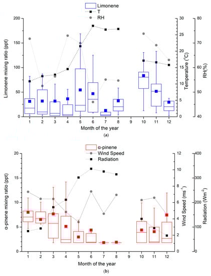
Figure 1.
Monthly average mixing ratios (in ppt) of (a) limonene and (b) α-pinene at Finokalia station from March 2014 to April 2015. Whiskers represent the 5th and 95th percentiles, box edges are the 25th and 75th percentiles, the line in the box is the median, the square is the mean of the reported values, and the mixing ratio is in ppt. The meteorological parameters (temperature, relative humidity, wind speed and radiation), averaged over the days of the samplings, are also depicted.
Limonene exhibits different behavior compared to α-pinene (Figure 1a) following the temperature and solar radiation variability, except in June/July/August when the temperature is high and the relative humidity is low. The mixing ratios of limonene at Finokalia are in consonance with the worldwide observations listed in Table 2 and the mean mixing ratio of these studies. However, the measurements in Portugal [26] and in a tropical forest [57] are two times higher than in Finokalia. The limonene observations at a Finnish boreal forest [23,24,38], varying from the LOD to 22 ppt, are lower than the observations at Finokalia. The limonene observations at Finokalia are of the same order of magnitude as the reported values for Corsica [57] and Cyprus [27] but are significantly lower than those observed in a temperate forest in Greece [56]. The limonene mixing ratios show a seasonal maximum during October with a mean value of 83.6 ppt. A secondary seasonal maximum can be seen during May, with a mean of 54.4 ppt. Ref. [58] reported that limonene was slightly more important in winter than summer in a suburban environment. Similarly, measurements in urban areas showed higher mixing ratios in winter than in summer for pinenes, which is potentially attributed to the anthropogenic sources of monoterpenes, such as traffic and wood combustion [19]. Ref. [52] observed that limonene in Helsinki was just as high in winter and autumn and higher in summer.
Table 2.
Comparison of this work with those reported in the literature: α-pinene, limonene and 1,8-cineol observations in different environments (with standard deviation when available) (mixing ratios in ppt). bdl: below detection limit.
Table 2.
Comparison of this work with those reported in the literature: α-pinene, limonene and 1,8-cineol observations in different environments (with standard deviation when available) (mixing ratios in ppt). bdl: below detection limit.
| Location | Type | Period | Method | Time | α-Pinene | Limonene | 1,8-Cineol | Reference |
|---|---|---|---|---|---|---|---|---|
| Anadia, Portugal | Rural | 12 & 24 August 1996 | GC-FID | day | 180 | 40 | 110 | Cerqueira et al. [26] |
| night | 460 | 73 | 270 | |||||
| Tábua, Portugal | Rural | 12 & 24 August 1996 | GC-FID | day | 190 | 30 | 260 | Cerqueira et al. [26] |
| night | 600 | 47 | 420 | |||||
| Peyrusse-Vieille, France | Rural | February–March & June–July 2009 | GC-FID-MS | winter | 16 | 30 | - | Detournay et al. [27] |
| summer | 102 | 20 | ||||||
| Peyrusse-Vieille, France | Rural | June–July 2009 | GC-FID-MS | 9-363 | LOD-66 | - | Detournay et al. [28] | |
| Hyytiälä, Finland | Boreal forest | April 2000–April 2002 | GC-MS | winter | 48 ± 46 | bdl | bdl | Hakola et al. [23] |
| spring | 62 ± 91 | bdl | bdl | |||||
| summer | 104 ± 54 | 13 ± 10 | 16 ± 13 | |||||
| autumn | 109 ± 88 | 13 ± 14 | bdl | |||||
| Hyytiälä, Finland | Boreal forest | 2000–2003 | GC-MS | winter | 52 | 0 | 2 | Hakola et al. [24] |
| spring | 69 | 0 | 1 | |||||
| summer | 107 | 0 | 24 | |||||
| autumn | 110 | 3 | 1 | |||||
| Hyytiälä, Finland | Boreal forest | October 2010–October 2011 | GC-MS | winter day | 6 | 2 | 1 | Hakola et al. [38] |
| winter afternoon | 5 | 3 | 1 | |||||
| spring day | 32 | 2 | 2 | |||||
| spring afternoon | 3 | 1 | 1 | |||||
| summer day | 189 | 22 | 9 | |||||
| summer afternoon | 71 | 7 | 12 | |||||
| autumn day | 38 | 4 | 2 | |||||
| autumn afternoon | 23 | 3 | 2 | |||||
| Helsinki, Finland | Urban | 2009 | GC-MS | winter | 15 | 8 | 1 | Hellén et al. [52] |
| spring | 17 | 3 | 2 | |||||
| summer | 58 | 11 | 8 | |||||
| autumn | 13 | 8 | 3 | |||||
| Borneo, Malaysian | Tropical forest | April–May & June-July 2008 | GC-FID | 24 | 71 | Jones et al. [57] | ||
| Amazonas, Brazil | Tropical forest | October 2015 | GC-FID | day | 330 ± 40 | 180 ± 90 | Yáñez-Serrano et al. [59] | |
| night | 150 ± 50 | 180 ± 100 | ||||||
| Athens, Greece | Urban | February 2016–February 2017 | GC-FID | winter | 120.5 ± 163.7 | 86.3 ± 190.6 | - | Panopoulou et al. [19] |
| summer | 125.9 ± 118.7 | 27.0 ± 55.8 | ||||||
| Paris, France | Suburban | July 2009 & January–February 2010 | GC-FID-MS | winter | 20 ± 52 | 15 ± 19 | W. Ait-Helal et al. [58] | |
| summer | 48 ± 45 | 16 ± 16 | ||||||
| Italy, Castelporziano | Rural | May–June 2007 | PRT-MS | 130–300 (monoterpenes) | Davinson et al. [35] | |||
| Greece, Pertouli | Temperate forest | July–August 1997 | GC-FID | summer | ≤2000 | ≤1500 | ≤500 | Harrison et al. [56] |
| Corsica | Coastal | June 2012–June 2014 | GC-FID | Annual | 68.3 ± 109.7 | 34.2 ± 54.0 | Debevec et al. [53] | |
| winter | 18.0 ± 18.0 | 18.0 ± 18.0 | ||||||
| spring | 54.0 ± 161.9 | 18.0 ± 71.9 | ||||||
| summer | 125.9 ± 89.9 | 71.9 ± 36.0 | ||||||
| autumn | 89.9 ± 89.9 | 54.0 ± 54.0 | ||||||
| Cyprus | Background rural | March 2015 | GC-FID | winter | 59.3 | Debevec et al. [54] | ||
| Cyprus | Forests and Macchia | March 2015 | GC-FID | 24 h | 58 ± 131 | 27 | Debevec et al. [55] | |
| Finokalia, Crete, Greece | Coastal | March 2014–April 2025 | GC-FID | winter | 7.5 ± 3.4 | 31.4 ± 37.9 | 11.5 ± 9 | This study |
| spring | 7.0 ± 9.8 | 33.3 ± 60.6 | 20.8 ± 21.6 | |||||
| March 2014–April 2025 | summer | 2.4 ± 3.0 | 24.1 ± 31.2 | bdl | ||||
| autumn | 5.1 ± 7.2 | 54.4 ± 41.2 | bdl |
At Finokalia, 1,8-cineol was detected only from January to March 2015 (mean of 16.3 ± 17.7 ppt), while it was below the LOD during the rest of the year. The mean value of 1,8-cineol compares well with the urban measurements at Helsinki in Finland [52] during winter and spring, when accounting that only 23% of the samples were containing 1,8-cineol above the LOD at Finokalia. The observations at the boreal forest in Finland are of the same order of magnitude as those in urban locations [24,38]. On the contrary, the measurements in Portugal during summer were comparing too high [26] and, together with those reported for the temperate forest in Greece [56], are the highest reported values.
Considering Finokalia’s location on a remote coast, with the nearest city being 50 km away, these data suggest that monoterpenes could originate from distant regional sources. Thus, further analysis of how the air mass origin influences the monoterpene concentrations is presented in Section 3.4. The lower values of monoterpenes at Finokalia in summer, compared to the other seasons, could also be attributed to stronger sinks in summer since OH radicals, which are mainly formed from the photolysis of O3 followed by the reaction of O1D with water vapor, are lower in winter when photochemical activity is low. Another reason for the high autumn and winter values is the seasonality of vegetation at Finokalia. The weather on the Island of Crete is characterized by two seasons: the wet season from October to March and the dry season from April to September. The wet season coincides with the green period at Finokalia; they both start in late autumn. During this period, phrygana vegetation grows because of the rainfall while the temperature is still high, as Finokalia is located in the southeast Mediterranean.
3.2. Monoterpene Diurnal Cycles
The diurnal patterns of the measured monoterpenes are presented in Figure 2. Concerning limonene, the highest mixing ratios were observed during autumn, with a diurnal magnitude of about 65 ppt (Figure 2a). For the following discussion, data are presented as a function of local wintertime, that is, UTC + 2. In autumn, high mixing ratios were observed in the afternoon, and a secondary morning maximum can be seen from 8:00 to 10:00. In winter, the diurnal variability is not that clear due to the low mixing ratios in the afternoon (around 17:00) and high mixing ratios in the early and late afternoon. Thus, during winter, a diurnal cycle with two maxima, one around 15:00 and the second in the evening (20:00 to 22:00), was generally observed. However, this is not the case for summer and spring when no specific diurnal circle was observed.
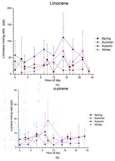
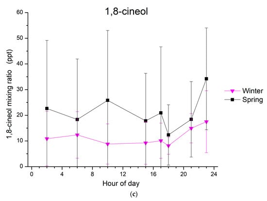
Figure 2.
Diurnal average variation in mixing ratios (in ppt) of (a) limonene, (b) α-pinene and (c) 1,8-cineol at Finokalia station during spring (in black), summer (in red), autumn (in blue) and winter (in purple) from March 2014 to April 2015; time is at local wintertime (UTC + 2). Whiskers represent the standard deviations.
For α-pinene, different diurnal patterns to those of limonene are observed (Figure 2b). During autumn, a clear diurnal cycle was seen with two maxima, the first one in the early morning (6:00 to 7:00) and the second one around noon (~12:00). This is not the case for winter, when only one maximum can be seen in the morning (9:00 to 10:00). During both spring and summer, the α-pinene mixing ratios present a clear diurnal variability, with an early morning maximum followed by an early afternoon minimum, reflecting the daytime oxidation of this monoterpene. Concerning 1,8-cineol, the mixing ratios that were detected above the LOD and observed from January to March 2015 do not show any clear variability.
The spring and summer diurnal patterns of α-pinene are similar to a typical cycle for biogenic compounds, with high levels at the beginning of the night and in the early morning, followed by an abrupt decrease around midday and a sharp increase again in the evening. High levels of monoterpenes are observed in the morning due to temperature-dependent emissions, which result in high emissions before the intense photochemical depletion processes occur (Figure 3). As shown in Figure 3a, the temperature is the highest in summer when relative humidity is the lowest (Figure 3c) and increases with increasing radiation (Figure 3b) in all seasons. During the day, the oxidizing capacity of the atmosphere is higher than during the night; therefore, the depletion processes surpass emission, leading to a rapid decline of monoterpene mixing ratios. Minimum mixing ratios coincide with the maximum photochemical activities. Regarding the nighttime increases, significant monoterpene emissions can still occur during the night, while the depletion of monoterpenes by chemical reactions with OH and O3, which maximize at noon and in the afternoon, respectively, declines when daylight and wind speeds are low. Changes in the height of the planetary boundary layer (PBL) at Finokalia station could not explain the limonene increase during the night, as the PBL at this site was observed to be dominated by coastal flows rather than thermal convection [60].
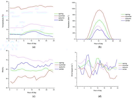
Figure 3.
Diurnal variability of (a) temperature, (b) solar radiation, (c) relative humidity and (d) wind speed near surface averaged over the days of the observations during each season from March 2014 to April 2015.
3.3. Factor Analysis-Source Identification
The exploration of potential sources of the observed monoterpenes in the region was performed based on a factor analysis that considers monoterpene observations together with the auxiliary measurements of other chemical parameters at Finokalia station (Table 3). No correlation was found with the meteorological parameters shown in Figure 3. In particular, Na+, NH4+, Mg++, Cl−, NO3−, SO4=, K+, Ca++ and C2O4= ions in the particulate phase and NH3, SO2, HCl and HNO3 in the gas phase were considered. Four-hour data were used in a varimax-rotated factor analysis since the monoterpene mixing ratios were averaged to the 4 h periods of the auxiliary observations. No 1,8-cineοl was included in our analysis since its mixing ratios were close to the LOD, and only a few samples were detected above the LOD from January to March 2015. Five common factors were found to be able to explain 85% of the total variance of the system (Table 3). Factor 1 is highly correlated with HCl, SO2, NO3−, SO4=, C2O4=, NH4+ and K+, which have an anthropogenic origin. This factor explains 35.5% of the total variance. Factor 2 is associated with Na+, Cl−, and Mg++, which are typical components of seawater and describe 23.9% of the system’s variability. Limonene has common sources with NH3, as these species are associated with Factor 3, which can reproduce 10.8% of the system’s variance. In Factor 4, which explains 8.2% of the total variance, α-pinene is associated with HNO3, suggesting that they have common sources. However, a source attribution of Factor 4 is difficult and could benefit from additional auxiliary observations. Finally, Ca++ is the only compound associated with Factor 5, which accounts for an additional 6.1% of the system’s variance.
Table 3.
Varimax-rotated factor matrix resulting from the factor analysis showing the correlations between atmospheric chemical components and factors.
The factor analysis showed that limonene and α-pinene have different sources in the region, while none of the observed monoterpenes was associated with the anthropogenic factor (Factor 1) nor the marine factor (Factor 2). Finokalia’s remote coastal location suggests that the station is subject to long-range transport of atmospheric constituents. The fact that monoterpenes are not related to Factor 1 (anthropogenic factor) shows that monoterpenes’ sources are local and are not related to the long-range transport of pollutants from urban environments.
The limonene and NH3 correlation with Factor 3 supports the existence of common sources of these compounds, most probably associated with the agricultural activities in the region. Such sources are known as major contributors (85–98%) to the NH3 emissions in the atmosphere [61].
3.4. Air Mass Back Trajectories Analysis
Air mass back-trajectory analysis was performed to investigate how the air mass origin influences the monoterpene mixing ratios. For this, five-day back-trajectories, arriving at Finokalia station at 1000 m a.s.l, were calculated by the HYSPLIT model (Hybrid Single-Particle Lagrangian Integrated Trajectory model) [62], following the methodology described in [44]. This height was chosen to avoid interferences in the calculations of the origin of the air masses by the orography of the island. To classify the back trajectories, we have defined and used eight sectors of air mass origin. The frequency of occurrence of the air mass origins for the analyzed samples was as follows: northern (N) (100 samples), northeastern (NE) (64 samples) and southwestern (SW) (54 samples). western (W), northwestern (NW), southern (S) and southeastern (SE) wind directions were observed only for 24, 23, 29 and 8 samples, respectively; no air mass of east (E) origin was sampled (Table 4).
Table 4.
Average monoterpene mixing ratios (standard deviation in parentheses) for each air mass sector; n is the number of samples per sector. The two largest mean mixing ratios are marked in bold.
The limonene and α-pinene mixing ratios were the highest in the air masses originating from the SW and NE and the lowest in the air masses originating from the SE. On the contrary, the 1,8-cineol maximum values were observed in W air masses (Table 4). Precisely, the average limonene mixing ratios equal to 46.2 ± 51.4 ppt, 42.0 ± 49.2 ppt, 35.3 ± 47 ppt, 30.9 ± 30.6 ppt and 25.3 ± 16.3 ppt were determined in the SW, NE, NW, N and S air masses, respectively. Limonene’s lowest values of 8.4 ppt were observed in the SE air masses. The mixing ratios of α-pinene were 8.0 ± 7.5 ppt, 7.8 ± 1.3 ppt, 6.7 ± 3.9 ppt, 5.4 ± 2.1 ppt, 5.2 ± 3.2 ppt and 4.5 ± 3.0 ppt for the NE, S, W, SW, N and NW air masses, respectively. Both limonene and α-pinene show low mixing ratios in the W air masses in contrast to 1,8-cineol, which shows its maximum mixing ratios equal to 22.4 ± 24.0 in the W air masses. For the rest of the wind sectors, the 1,8-cineol average mixing ratios are quite similar, with 12.7 ± 10.7 ppt, 12.3 ± 18.3 ppt, 11.8 ± 13.2 ppt, 10.2 ± 12.8 ppt and 6.2 ± 1.8 ppt for the NW, NE, SW, N and S wind directions, respectively. The large variability of monoterpene mixing ratios within each sector, depicted by the standard deviation of the observations, prohibits any firm conclusion.
3.5. Monoterpenes and NPF
The potential participation of monoterpenes in nucleation events in our region has been investigated based on the NPF events at Finokalia (Figure 4) and identified the following [51] based on the measured aerosol particle size distributions from 13 March 2014 to 20 April 2015. Days were classified as ‘NPF event days’ when a new nucleation mode followed by growth to larger diameters was clearly observed after manual inspection [46].
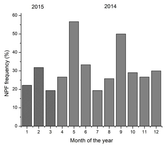
Figure 4.
Monthly percentage frequency of occurrence of NPF at Finokalia station from March 2014 to March 2015 (full months are presented). Shaded columns indicate data from 2015.
Most NPF events were observed in spring (May) and fall (September). As pointed out earlier, limonene’s seasonality clearly shows a seasonal maximum in October and a secondary seasonal maximum in May. This suggests the potential existence of a link between the NPF events and the high limonene mixing ratios in May, and thus that limonene may contribute to the production of new particles. Regarding the seasonal maximum of the NPF events in September, the lack of monoterpene measurements in this month does not allow for a comparison with them and requires further investigation.
4. Conclusions
A one-year-long observation of monoterpenes in the Eastern Mediterranean at Finokalia is presented here. The station is a remote coastal site characterized mainly by the typical phrygana vegetation of Crete, where shrubs and degraded macchia-type vegetation dominate the landscape. A total of 345 samples were collected from March 2014 to April 2015 during three intensive campaigns and a systematic collection of one diurnal cycle per week. Air samples were collected in absorption tubes and analyzed offline using a GC–FID system.
The most abundant monoterpene was limonene, with its highest mixing ratios observed in spring and autumn in contrast to the earlier reported studies that showed a summer maximum indicative of biogenic sources. Similarly, the mixing ratios of α-pinene were maximized in winter and spring and minimized in summer. These differences could be due to (i) a stronger photochemical sink in summer and (ii) the different vegetation seasonal cycle with the green period at Finokalia starting in late autumn.
A clear diurnal cycle of α-pinene was observed during spring and summer, with a minimum around noon that reflected its photochemical loss. This diurnal pattern is quite typical for biogenic compounds where minimum mixing ratios coincide with maximum photochemical activity. However, in our study, the monoterpene mixing ratios did not statistically correlate with the meteorological parameters.
The factor analysis showed that limonene and α-pinene have different sources and suggested that none of the studied monoterpenes correlates with the anthropogenic sources. No clear dependence of monoterpene mixing ratios on air mass origin was found. Furthermore, a similarity was detected between the seasonality of the limonene mixing ratios and NPF events’ frequency of occurrence with maxima during spring, indicating that limonene may contribute to the NPF procedure. However, the lack of measurements of monoterpene mixing ratios in September, when the NPF events occurrence presents a second maximum, does not allow us to draw an overall conclusion and further investigation is needed. This paper presented offline measurements that demonstrated the presence of monoterpenes in the remote background atmosphere of the Eastern Mediterranean and the need for new continuous online simultaneous observations of monoterpenes and aerosol size distribution in the region. Such observations are ongoing and will provide more robust information on the involvement of these organics in aerosol formation and growth.
Author Contributions
Conceptualization, Μ.Κ. and Ν.Κ.; methodology, Ε.Τ., G.K. and N.M.; software, Ε.Τ.; validation, Ε.Τ. and G.Κ.; formal analysis, Ε.Τ. and G.K.; writing—original draft preparation, E.T.; writing—review and editing, M.K. and N.K.; visualization, Ν.Κ.; supervision, Μ.Κ.; funding acquisition, N.K. and M.K. All authors have read and agreed to the published version of the manuscript.
Funding
We acknowledge the support of this work by the project “PANhellenic infrastructure for Atmospheric Composition and climatE change” (MIS 5021516), which is implemented under the action “Reinforcement of the Research and Innovation Infrastructure”, funded by the operational programme “Competitiveness, Entrepreneurship and Innovation” (NSRF 2014–2020) and co-financed by Greece and the European Union (European Regional Development Fund) and the HORIZON project Edu4Climate n. 101071247. MK acknowledges support from the Deutsche Forschungsgemeinschaft (DFG, German Research Foundation) under Germany’s Excellence Strategy (University Allowance, EXC 2077, University of Bremen).
Institutional Review Board Statement
Not applicable.
Informed Consent Statement
Not applicable.
Data Availability Statement
The data are available from the corresponding author upon request.
Acknowledgments
We thank the reviewers for their comments that helped improve the presentation of the manuscript.
Conflicts of Interest
The authors declare no conflict of interest.
References
- Sillman, S. The Relation between Ozone, NOx and Hydrocarbons in Urban and Polluted Rural Environments. Atmos. Environ. 1999, 33, 1821–1845. [Google Scholar] [CrossRef]
- Kleinman, L. The Dependence of Tropospheric Ozone Production Rate on Ozone Precursors. Atmos. Environ. 2005, 39, 575–586. [Google Scholar] [CrossRef]
- Kulmala, M.; Kerminen, V.-M.; Anttila, T.; Laaksonen, A.; O’Dowd, C.D. Organic Aerosol Formation via Sulphate Cluster Activation. J. Geophys. Res. Atmos. 2004, 109, D04205. [Google Scholar] [CrossRef]
- Tunved, P.; Hansson, H.-C.; Kerminen, V.-M.; Ström, J.; Maso, M.D.; Lihavainen, H.; Viisanen, Y.; Aalto, P.P.; Komppula, M.; Kulmala, M. High Natural Aerosol Loading over Boreal Forests. Science 2006, 312, 261–263. [Google Scholar] [CrossRef]
- Bonn, B.; Kulmala, M.; Riipinen, I.; Sihto, S.-L.; Ruuskanen, T.M. How Biogenic Terpenes Govern the Correlation between Sulfuric Acid Concentrations and New Particle Formation. J. Geophys. Res. Atmos. 2008, 113, D1220. [Google Scholar] [CrossRef]
- Climate Forcing Due to Tropospheric and Stratospheric Ozone. J. Geophys. Res. Atmos. 1999, 104, 31239–31254. [CrossRef]
- Fowler, D.; Pilegaard, K.; Sutton, M.A.; Ambus, P.; Raivonen, M.; Duyzer, J.; Simpson, D.; Fagerli, H.; Fuzzi, S.; Schjoerring, J.K.; et al. Atmospheric Composition Change: Ecosystems–Atmosphere Interactions. Atmos. Environ. 2009, 43, 5193–5267. [Google Scholar] [CrossRef]
- Lippmann, M. Health Effects of Ozone. A Critical Review. JAPCA 1989, 39, 672–695. [Google Scholar] [CrossRef]
- Kalkavouras, P.; Bougiatioti, A.; Kalivitis, N.; Stavroulas, I.; Tombrou, M.; Nenes, A.; Mihalopoulos, N. Regional New Particle Formation as Modulators of Cloud Condensation Nuclei and Cloud Droplet Number in the Eastern Mediterranean. Atmos. Chem. Phys. 2019, 19, 6185–6203. [Google Scholar] [CrossRef]
- EEA Air Quality in Europe 2022—Report, No. 05/2022; 2022.
- Guenther, A.; Karl, T.; Harley, P.; Wiedinmyer, C.; Palmer, P.I.; Geron, C. Estimates of Global Terrestrial Isoprene Emissions Using MEGAN (Model of Emissions of Gases and Aerosols from Nature). Atmos. Chem. Phys. 2006, 6, 3181–3210. [Google Scholar] [CrossRef]
- Bourtsoukidis, E.; Pozzer, A.; Williams, J.; Makowski, D.; Penuelas, J.; Matthaios, V.; Lazoglou, G.; Yañez-Serrano, A.; Ciais, P.; Lelieveld, J.; et al. High Temperature Sensitivity of Monoterpene Emissions from Global Vegetation. Res. Sq. 2022. in preprint. [Google Scholar] [CrossRef]
- Peñuelas, J.; Llusià, J.; Asensio, D.; Munné-Bosch, S. Linking Isoprene with Plant Thermotolerance, Antioxidants and Monoterpene Emissions. Plant. Cell Environ. 2005, 28, 278–286. [Google Scholar] [CrossRef]
- Peñuelas, J.; Munné-Bosch, S. Isoprenoids: An Evolutionary Pool for Photoprotection. Trends Plant Sci. 2005, 10, 166–169. [Google Scholar] [CrossRef] [PubMed]
- Peñuelas, J.; Llusià, J. Linking Photorespiration, Monoterpenes and Thermotolerance in Quercus. New Phytol. 2002, 155, 227–237. [Google Scholar] [CrossRef]
- Kegge, W.; Pierik, R. Biogenic Volatile Organic Compounds and Plant Competition. Trends Plant Sci. 2010, 15, 126–132. [Google Scholar] [CrossRef] [PubMed]
- Wright, G.A.; Schiestl, F.P. The Evolution of Floral Scent: The Influence of Olfactory Learning by Insect Pollinators on the Honest Signalling of Floral Rewards. Funct. Ecol. 2009, 23, 841–851. [Google Scholar] [CrossRef]
- Dai, T.; Wang, W.; Ren, L.; Chen, J.; Liu, H. Emissions of Non-Methane Hydrocarbons from Cars in China. Sci. China Chem. 2010, 53, 263–272. [Google Scholar] [CrossRef]
- Panopoulou, A.; Liakakou, E.; Sauvage, S.; Gros, V.; Locoge, N.; Stavroulas, I.; Bonsang, B.; Gerasopoulos, E.; Mihalopoulos, N. Yearlong Measurements of Monoterpenes and Isoprene in a Mediterranean City (Athens): Natural vs. Anthropogenic Origin. Atmos. Environ. 2020, 243, 117803. [Google Scholar] [CrossRef]
- McDonald, B.C.; de Gouw, J.A.; Gilman, J.B.; Jathar, S.H.; Akherati, A.; Cappa, C.D.; Jimenez, J.L.; Lee-Taylor, J.; Hayes, P.L.; McKeen, S.A.; et al. Volatile Chemical Products Emerging as Largest Petrochemical Source of Urban Organic Emissions. Science 2018, 359, 760–764. [Google Scholar] [CrossRef]
- Pallozzi, E.; Lusini, I.; Cherubini, L.; Hajiaghayeva, R.A.; Ciccioli, P.; Calfapietra, C. Differences between a Deciduous and a Conifer Tree Species in Gaseous and Particulate Emissions from Biomass Burning. Environ. Pollut. 2018, 234, 457–467. [Google Scholar] [CrossRef]
- Simpson, I.J.; Blake, N.J.; Barletta, B.; Diskin, G.S.; Fuelberg, H.E.; Gorham, K.; Huey, L.G.; Meinardi, S.; Rowland, F.S.; Vay, S.A.; et al. Characterization of Trace Gases Measured over Alberta Oil Sands Mining Operations: 76 Speciated C2–C10 Volatile Organic Compounds (VOCs), CO2, CH4, CO, NO, NO2, NOy, O3 and SO2. Atmos. Chem. Phys. 2010, 10, 11931–11954. [Google Scholar] [CrossRef]
- Hakola, H.; Tarvainen, V.; Laurila, T.; Hiltunen, V.; Hellén, H.; Keronen, P. Seasonal Variation of VOC Concentrations above a Boreal Coniferous Forest. Atmos. Environ. 2003, 37, 1623–1634. [Google Scholar] [CrossRef]
- Hakola, H.; Hellén, H.; Tarvainen, V.; Bäck, J.; Patokoski, J.; Rinne, J.; Hakola, H.; Tarvainen, H.; Bäck, V. Annual Variations of Atmospheric VOC Concentrations in a Boreal Forest. Boreal Environ. Res. 2009, 14, 722–730. [Google Scholar]
- Kesselmeier, J.; Kuhn, U.; Wolf, A.; Andreae, M.O.; Ciccioli, P.; Brancaleoni, E.; Frattoni, M.; Guenther, A.; Greenberg, J.; De Castro Vasconcellos, P.; et al. Atmospheric Volatile Organic Compounds (VOC) at a Remote Tropical Forest Site in Central Amazonia. Atmos. Environ. 2000, 34, 4063–4072. [Google Scholar] [CrossRef]
- Cerqueira, M.A.; Pio, C.A.; Gomes, P.A.; Matos, J.S.; Nunes, T. V Volatile Organic Compounds in Rural Atmospheres of Central Portugal. Sci. Total Environ. 2003, 313, 49–60. [Google Scholar] [CrossRef] [PubMed]
- Detournay, A.; Sauvage, S.; Locoge, N.; Gaudion, V.; Leonardis, T.; Fronval, I.; Kaluzny, P.; Galloo, J.-C. Development of a Sampling Method for the Simultaneous Monitoring of Straight-Chain Alkanes, Straight-Chain Saturated Carbonyl Compounds and Monoterpenes in Remote Areas. J. Environ. Monit. 2011, 13, 983–990. [Google Scholar] [CrossRef]
- Detournay, A.; Sauvage, S.; Riffault, V.; Wroblewski, A.; Locoge, N. Source and Behavior of Isoprenoid Compounds at a Southern France Remote Site. Atmos. Environ. 2013, 77, 272–282. [Google Scholar] [CrossRef]
- Rinne, J.; Ruuskanen, T.; Reissell, A.; Taipale, R.; Hakola, H.; Kulmala, M. On-Line PTR-MS Measurements of Atmospheric Concentrations of Volatile Organic Compounds in a European Boreal Forest Ecosystem. Boreal Environ. Res. 2005, 10, 425. [Google Scholar]
- Lappalainen, H.K.; Sevanto, S.; Bäck, J.; Ruuskanen, T.M.; Kolari, P.; Taipale, R.; Rinne, J.; Kulmala, M.; Hari, P. Day-Time Concentrations of Biogenic Volatile Organic Compounds in a Boreal Forest Canopy and Their Relation to Environmental and Biological Factors. Atmos. Chem. Phys. 2009, 9, 5447–5459. [Google Scholar] [CrossRef]
- Spirig, C.; Neftel, A.; Ammann, C.; Dommen, J.; Grabmer, W.; Thielmann, A.; Schaub, A.; Beauchamp, J.; Wisthaler, A.; Hansel, A. Eddy Covariance Flux Measurements of Biogenic VOCs during ECHO 2003 Using Proton Transfer Reaction Mass Spectrometry. Atmos. Chem. Phys. 2005, 5, 465–481. [Google Scholar] [CrossRef]
- Jordan, C.; Fitz, E.; Hagan, T.; Sive, B.; Frinak, E.; Haase, K.; Cottrell, L.; Buckley, S.; Talbot, R. Long-Term Study of VOCs Measured with PTR-MS at a Rural Site in New Hampshire with Urban Influences. Atmos. Chem. Phys. 2009, 9, 4677–4697. [Google Scholar] [CrossRef]
- Fortner, E.C.; Zheng, J.; Zhang, R.; Berk Knighton, W.; Volkamer, R.M.; Sheehy, P.; Molina, L.; André, M. Measurements of Volatile Organic Compounds Using Proton Transfer Reaction—Mass Spectrometry during the MILAGRO 2006 Campaign. Atmos. Chem. Phys. 2009, 9, 467–481. [Google Scholar] [CrossRef]
- Filella, I.; Penuelas, J. Daily, Weekly, and Seasonal Time Courses of VOC Concentrations in a Semi-Urban Area Near Barcelona. Atmos. Environ. 2006, 40, 7752–7769. [Google Scholar] [CrossRef]
- Davison, B.; Taipale, R.; Langford, B.; Misztal, P.; Fares, S.; Matteucci, G.; Loreto, F.; Cape, J.N.; Rinne, J.; Hewitt, C.N. Concentrations and Fluxes of Biogenic Volatile Organic Compounds above a Mediterranean Macchia Ecosystem in Western Italy. Biogeosciences 2009, 6, 1655–1670. [Google Scholar] [CrossRef]
- Seco, R.; Peñuelas, J.; Filella, I.; Llusià, J.; Molowny-Horas, R.; Schallhart, S.; Metzger, A.; Müller, M.; Hansel, A. Contrasting Winter and Summer VOC Mixing Ratios at a Forest Site in the Western Mediterranean Basin: The Effect of Local Biogenic Emissions. Atmos. Chem. Phys. 2011, 11, 13161–13179. [Google Scholar] [CrossRef]
- Cheng, X.; Li, H.; Zhang, Y.; Li, Y.; Zhang, W.; Wang, X.; Bi, F.; Zhang, H.; Gao, J.; Chai, F.; et al. Atmospheric Isoprene and Monoterpenes in a Typical Urban Area of Beijing: Pollution Characterization, Chemical Reactivity and Source Identification. J. Environ. Sci. 2018, 71, 150–167. [Google Scholar] [CrossRef]
- Hakola, H.; Hellén, H.; Hemmilä, M.; Rinne, J.; Kulmala, M. In Situ Measurements of Volatile Organic Compounds in a Boreal Forest. Atmos. Chem. Phys. 2012, 12, 11665–11678. [Google Scholar] [CrossRef]
- Schade, G.W.; Goldstein, A.H. Increase of Monoterpene Emissions from a Pine Plantation as a Result of Mechanical Disturbances. Geophys. Res. Lett. 2003, 30, 1380. [Google Scholar] [CrossRef]
- Noe, S.M.; Peñuelas, J.; Niinemets, U. Monoterpene Emissions from Ornamental Trees in Urban Areas: A Case Study of Barcelona, Spain. Plant Biol. 2008, 10, 163–169. [Google Scholar] [CrossRef]
- Atkinson, R.; Arey, J. Gas-Phase Tropospheric Chemistry of Biogenic Volatile Organic Compounds: A Review. Atmos. Environ. 2003, 37, 197–219. [Google Scholar] [CrossRef]
- The Physical Science Basis. Summary for Policymakers. In IPCC 2022: Climate Change 2022; Masson-Delmotte, B.Z., Zhai, V.P., Pirani, A., Connors, S.L., Péan, C., Berger, S., Caud, N., Chen, Y., Goldfarb, L., Gomis, M.I., et al., Eds.; Cambridge University Press: Cambridge, UK; New York, NY, USA, 2022; Available online: https://www.klimamanifest-von-heiligenroth.de/wp/wp-content/uploads/2014/02/IPCC2013_WG1AR5_ALL_FINAL_S768_14Grad_mitTitelCover.pdf (accessed on 16 February 2023).
- Seco, R.; Peñuelas, J.; Filella, I.; Llusia, J.; Schallhart, S.; Metzger, A.; Müller, M.; Hansel, A. Volatile Organic Compounds in the Western Mediterranean Basin: Urban and Rural Winter Measurements during the DAURE Campaign. Atmos. Chem. Phys. 2013, 13, 4291–4306. [Google Scholar] [CrossRef]
- Mihalopoulos, N.; Stephanou, E.; Kanakidou, M.; Pilitsidis, S.; Bousquet, P. Tropospheric Aerosol Ionic Composition in the Eastern Mediterranean Region. Tellus B 1997, 49, 314–326. [Google Scholar] [CrossRef]
- Lelieveld, J.; Berresheim, H.; Borrmann, S.; Crutzen, P.J.; Dentener, F.J.; Fischer, H.; Feichter, J.; Flatau, P.J.; Heland, J.; Holzinger, R.; et al. Global Air Pollution Crossroads over the Mediterranean. Science 2002, 298, 794–799. [Google Scholar] [CrossRef] [PubMed]
- Kalivitis, N.; Kerminen, V.-M.; Kouvarakis, G.; Stavroulas, I.; Tzitzikalaki, E.; Kalkavouras, P.; Daskalakis, N.; Myriokefalitakis, S.; Bougiatioti, A.; Manninen, H.E.; et al. Formation and Growth of Atmospheric Nanoparticles in the Eastern Mediterranean: Results from Long-Term Measurements and Process Simulations. Atmos. Chem. Phys. 2019, 19, 2671–2686. [Google Scholar] [CrossRef]
- EPA Method TO-1. In U.S. EPA Technical Assistance Document; 1984; Volume 34.
- Woolfenden, E.A.; McClenny, W.A. Method TO-17 Determination of Volatile Organic Compounds in Ambient Air Using Active Sampling Onto Sorbent Tubes. In Compendium of Methods for the Determination of Toxic Organic Compounds in Ambient Air Second Edition Compendium; Manning, J.A., Burckle, J.O., Hedges, S., McElroy, F.F., Eds.; Center for Environmental Research Information Office of Research and Development U.S. Environmental Protection Agency: Cincinnati, OH, USA, 1999; EPA/625/R-; pp. 17–49. [Google Scholar]
- Tzitzikalaki, E.; Kalivitis, N.; Panagiotopoulou, G.; Kanakidou, M. Observations of Alkylamines in the East Mediterranean Atmosphere. In Proceedings of the 15th International Conference on Meteorology, Climatology and Atmospheric Physics COMECAP, Ioannina, Greece, 26–29 September 2021; Bartzokas, A., Nastos, P., Eds.; Hellenic Meteorological Society: Ioannina, Greece, 2021; pp. 185–189. [Google Scholar]
- Paraskevopoulou, D.; Liakakou, E.; Gerasopoulos, E.; Mihalopoulos, N. Sources of Atmospheric Aerosol from Long-Term Measurements (5 years) of Chemical Composition in Athens, Greece. Sci. Total Environ. 2015, 527–528, 165–178. [Google Scholar] [CrossRef]
- Dal Maso, M.; Kulmala, M.; Riipinen, I.; Wagner, R. Formation and Growth of Fresh Atmospheric Aerosols: Eight Years of Aerosol Size Distribution Data from SMEAR II, Hyytiälä, Finland. Boreal Environ. Res. 2005, 10, 323–336. [Google Scholar]
- Hellén, H.; Tykkä, T.; Hakola, H. Importance of Monoterpenes and Isoprene in Urban Air in Northern Europe. Atmos. Environ. 2012, 59, 59–66. [Google Scholar] [CrossRef]
- Debevec, C.; Sauvage, S.; Gros, V.; Salameh, T.; Sciare, J.; Dulac, F.; Locoge, N. Seasonal Variation and Origins of Volatile Organic Compounds Observed during 2 Years at a Western Mediterranean Remote Background Site (Ersa, Cape Corsica). Atmos. Chem. Phys. 2021, 21, 1449–1484. [Google Scholar] [CrossRef]
- Debevec, C.; Sauvage, S.; Gros, V.; Sciare, J.; Pikridas, M.; Stavroulas, I.; Salameh, T.; Leonardis, T.; Gaudion, V.; Depelchin, L.; et al. Origin and Variability in Volatile Organic Compounds Observed at an Eastern Mediterranean Background Site (Cyprus). Atmos. Chem. Phys. 2017, 17, 11355–11388. [Google Scholar] [CrossRef]
- Debevec, C.; Sauvage, S.; Gros, V.; Sellegri, K.; Sciare, J.; Pikridas, M.; Stavroulas, I.; Leonardis, T.; Gaudion, V.; Depelchin, L.; et al. Driving Parameters of Biogenic Volatile Organic Compounds and Consequences on New Particle Formation Observed at an Eastern Mediterranean Background Site. Atmos. Chem. Phys. 2018, 18, 14297–14325. [Google Scholar] [CrossRef]
- Harrison, D.; Hunter, M.C.; Lewis, A.C.; Seakins, P.W.; Bonsang, B.; Gros, V.; Kanakidou, M.; Touaty, M.; Kavouras, I.; Mihalopoulos, N.; et al. Ambient Isoprene and Monoterpene Concentrations in a Greek Fir (Abies Borisii-Regis) Forest. Reconciliation with Emissions Measurements and Effects on Measured OH Concentrations. Atmos. Environ. 2001, 35, 4699–4711. [Google Scholar] [CrossRef]
- Jones, C.; Hopkins, J.; Lewis, A. In Situ Measurements of Isoprene and Monoterpenes within a South-East Asian Tropical Rainforest. Atmos. Chem. Phys. Discuss. 2011, 11, 6971–6984. [Google Scholar] [CrossRef]
- Ait-Helal, W.; Borbon, A.; Sauvage, S.; de Gouw, J.A.; Colomb, A.; Gros, V.; Freutel, F.; Crippa, M.; Afif, C.; Baltensperger, U.; et al. Volatile and Intermediate Volatility Organic Compounds in Suburban Paris: Variability, Origin and Importance for SOA Formation. Atmos. Chem. Phys. 2014, 14, 10439–10464. [Google Scholar] [CrossRef]
- Yáñez-Serrano, A.M.; Nölscher, A.C.; Bourtsoukidis, E.; Gomes Alves, E.; Ganzeveld, L.; Bonn, B.; Wolff, S.; Sa, M.; Yamasoe, M.; Williams, J.; et al. Monoterpene Chemical Speciation in a Tropical Rainforest:Variation with Season, Height, and Time of Dayat the Amazon Tall Tower Observatory (ATTO). Atmos. Chem. Phys. 2018, 18, 3403–3418. [Google Scholar] [CrossRef]
- Tsikoudi, I.; Marinou, E.; Vakkari, V.; Gialitaki, A.; Tsichla, M.; Amiridis, V.; Komppula, M.; Raptis, I.P.; Kampouri, A.; Daskalopoulou, V.; et al. PBL Height Retrievals at a Coastal Site Using Multi-Instrument Profiling Methods. Remote Sens. 2022, 14, 4057. [Google Scholar] [CrossRef]
- Hertel, O.; Skjøth, C.; Reis, S.; Bleeker, A.; Harrison, R.; Cape, J.N.; Fowler, D.; Skiba, U.; Simpson, D.; Jickells, T.; et al. Governing Processes for Reactive Nitrogen Compounds in the European Atmosphere. Biogeosciences 2012, 9, 4921–4954. [Google Scholar] [CrossRef]
- Draxler, R.; Hess, G. An Overview of the HYSPLIT_4 Modeling System for Trajectories, Dispersion, and Deposition. Aust. Meteorol. Mag. 1998, 47, 295–308. [Google Scholar]


Disclaimer/Publisher’s Note: The statements, opinions and data contained in all publications are solely those of the individual author(s) and contributor(s) and not of MDPI and/or the editor(s). MDPI and/or the editor(s) disclaim responsibility for any injury to people or property resulting from any ideas, methods, instructions or products referred to in the content. |
© 2023 by the authors. Licensee MDPI, Basel, Switzerland. This article is an open access article distributed under the terms and conditions of the Creative Commons Attribution (CC BY) license (https://creativecommons.org/licenses/by/4.0/).