Spatiotemporal Analysis of NH₃ Emission Sources and Their Relation to Land Use Types in the Eastern German Lowlands

Abstract

Ammonia (NH₃) emissions, which are key precursors of fine particulate matter, pose significant environmental challenges. This study investigated the spatiotemporal variations in NH₃ emissions across the eastern German lowlands from 2013 to 2022 using IASI-B satellite data. Five major Land Cover Classes (LCC) –tree, grassland, cropland, built-up areas, and water bodies– were analyzed. The results showed distinct diurnal variations, with nighttime NH₃ concentrations exceeding 2.0 × 10¹⁶ molecules cm⁻² in the peak months. Seasonal patterns indicated significant emissions in March (1.2 × 10¹⁶ molecules cm⁻²), April (1.1 × 10¹⁶ molecules cm⁻²), and August (9.6 × 10¹⁵ molecules cm⁻²), while the lowest concentrations occurred in September (0.6 × 10¹⁵ molecules cm⁻²). Persistent hotspots were identified in the northwestern region, where emissions peaked in spring (1.8 × 10¹⁶ molecules cm⁻²⁾ and summer (1.3 × 10¹⁶ molecules cm⁻²), primarily due to agricultural activities. Over the study period, the annual NH₃ concentration peaked in 2015, 2018, and 2022. Using k-means clustering, three distinct emission zones were identified, with Cluster 3 showing the highest NH₃ emission values, particularly in urban centers, and agricultural zones were identified, covering less than 20% of the study area, where cropland predominates (8%). Meteorological factors significantly influenced NH₃ levels, with negative correlations obtained for precipitation, wind speed, and evaporation, while solar radiation, boundary layer height, and instantaneous moisture fluxes showed positive correlations. A case study from March 2022, employing the HYSPLIT trajectory model, confirmed that agricultural practices are the dominant NH₃ source, with emissions reaching 3.2 × 10¹⁶ molecules cm⁻² in hotspot regions.

1. Introduction

Ammonia (NH₃) in the atmosphere significantly impacts air quality and biodiversity through its long-range dispersion and interaction with meteorological conditions [1]. It is the primary alkaline constituent of the Earth’s atmosphere and a major precursor to the formation of fine aerosol particulate matter (PM_2.5), which consists of fine particulate matter with an aerodynamic diameter ≤2.5 µm [2,3], thus contributing to increasing mortality from respiratory and cardiovascular diseases [2,3,4,5,6]. NH₃ also plays a crucial role in the nitrogen (N) cycle and various biogeochemical processes as a reactive nitrogen species (Nr), serving as the main form of N in the environment [7,8]. Although NH₃ has a relatively temporary residence atmospheric lifetime–ranging from hours to a few days–due to its efficient deposition and rapid conversion to particles, current surface measurements are unable to reliably estimate global emissions without introducing substantial uncertainty [9,10]. Despite its critical role in atmosphere chemistry, significant uncertainties remain regarding its global distribution, source, transport, and dispersion. These uncertainties stem primarily from the limitations of ground-based monitoring methods, which are often insufficient for capturing significant fluctuations in NH₃ concentrations [7,11].

Due to its alkalinity, NH₃ readily reacts with acid-forming compounds, such as sulfur dioxide (SO₂) and nitrogen oxides (NO_x), in the atmosphere, leading to the formation of particles containing ammonium sulfate [(NH₄)₂SO₄] and ammonium nitrate [(NH₄)₂NO₃] particles [12,13]. The presence of these fine particulate matter (PM_2.5) components degrades air quality [14] and contributes to environmental effects by influencing the Earth’s radiation balance, reflecting sunlight, and affecting cloud properties [15]. During winter haze events, cold and humid conditions further promote the formation of ammonium nitrate [16]. Excessive NH₃ deposition in various ecosystems can lead to soil acidification, water eutrophication, and biodiversity loss [1,17,18]. The role of NH₃ in fine particulate formation poses substantial health risks, as extensive research has demonstrated that exposure to PM_2.5 is associated with increased hospital admissions, higher rates of cardiovascular and respiratory diseases, and increased overall mortality [19].

A widely used approach for monitoring and analyzing NH₃ spatiotemporal patterns is through satellite-based methods [20]. This technique utilizes satellite-based sensors to detect and measure atmospheric NH₃ concentrations, providing valuable insights into its spatial distribution and temporal variations. Ground-based monitoring is often limited by technical challenges and the high variability of NH₃ concentrations across time and space [7]. In contrast, satellite-based remote sensing offers comprehensive global coverage and high temporal resolution, allowing for continuous monitoring of NH₃ distribution and bridging the gaps in ground-based measurements. Satellite instruments detect NH₃ by measuring the infrared radiation emitted by the gas in the Earth’s atmosphere, enabling continuous monitoring of its spatial and temporal variability [7,21].

Several studies have successfully applied remote sensing to monitor NH₃ emissions. Clarisse et al. [22] used Infrared Atmospheric Sounding Interferometers (IASI) to observe NH₃ over Europe and demonstrate the capability to detect ammonia emission on a regional scale. Similarly, Van Damme et al. [23] employed IASI to analyze the global NH₃ distribution, revealing significant spatial variability, with the highest concentrations occurring in agricultural regions worldwide. Their findings underscored the importance of agricultural activities as a major source of NH₃ and demonstrated the effectiveness of the IASI in capturing global emission patterns. Remote sensing has also been useful for studying NH₃ emissions from agricultural activities [24,25,26,27,28] and monitoring NH₃ emissions from wildfires [29,30].

The agricultural sector, particularly livestock farming, is the primary source of NH₃ emissions in Europe, accounting for approximately 94% of total emissions [31]. In Germany, the average annual NH₃ emissions over the past decade have been estimated to be around 600 gigagrams (Gg) [32]. Although emissions have slightly declined over the last seven years, they continue to surpass the NH₃ threshold of 550 Gg established in air quality legislation [24,32,33,34]. This persistent exceedance points to the ongoing challenges in mitigating NH₃ emissions from agricultural practices despite regulatory efforts and highlights the need for land-use-related analysis of NH₃ distributions. In the livestock sector, manure management and the application of synthetic fertilizers contribute significantly to NH₃ emissions [33,34,35]. Emissions from cattle farming alone represent around 50% of the total agricultural NH₃ emissions, followed by pig and poultry farming, which together contribute an additional 30% [32,36]. The volatilization of NH₃ from livestock manure is highly dependent on environmental factors, such as temperature, humidity, and wind speed, which influence emission rates and atmospheric dispersion patterns [33].

Furthermore, NH₃ emission exhibits seasonal variations due to changes in agricultural practices. Peak emissions typically occur during Spring and Summer, coinciding with manure spreading and warmer temperatures that accelerate volatilization [24]. In contrast, emissions are relatively low in winter due to reduced microbial activity and less manure application [25,31,36]. These variations are critical for understanding NH_3, where intensive agricultural activities play a significant role in the emission dynamics.

The spatiotemporal dynamics of NH₃ emissions can be effectively analyzed in the eastern German lowlands, which are characterized by heterogeneous land use patterns and a predominantly agricultural landscape. The combination of intensive agricultural activities and diverse land use provides an ideal setting for studying the interactions between land use and NH₃ emission patterns, particularly in relation to local meteorological conditions [24,32,33,34]. Moreover, given the proximity of this region to urban centers such as Berlin, understanding NH₃ dispersion and transport is critical for managing emissions in nearby, densely populated areas.

This study focuses on NH₃ emissions in the eastern German lowlands, specifically within the administrative boundaries of Brandenburg, to ensure consistency in the analysis. The main objective of this study is to detect and analyze NH₃ emission sources in Brandenburg over space and time related to different land use types. This is achieved by utilizing NH₃ concentration data obtained through remote sensing and applying machine learning techniques. The analysis includes an evaluation of the spatiotemporal distribution of NH₃ concentration, identification of emission hotspot areas, and an assessment of the environmental factors influencing these patterns, including key meteorological variables. Additionally, NH₃ emissions are examined for various land use types, and the contribution of local and non-local sources to NH₃ levels is determined using back-trajectory dispersion modeling. The study is based on reanalyzed satellite remote sensing data from the IASI over 10 years (2013–2022) [7,37,38]. The central hypothesis is that NH₃ concentrations differ significantly between agricultural and non-agricultural land use types and are influenced by meteorological conditions. The study examines annual and seasonal cycles, with particular emphasis on variations across different seasons.

2. Materials and Methods

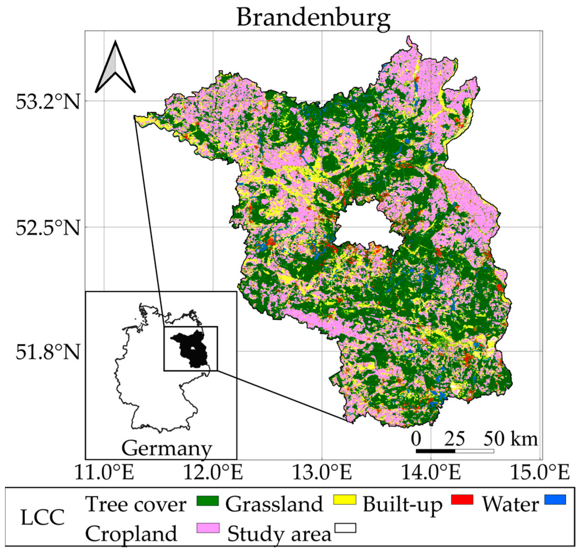
2.1. Study Area

The selected study area, Brandenburg, is located in the eastern German lowlands, spanning 51.3° N to 53.6° N and 11.4° E to 14.6° E. It covers 29,640 km² with a north–south extension of 244 km and an east–west extension of 234 km. Approximately 48.65% of its area comprises agricultural land, and 6.87% is covered by urban areas [39,40,41,42]. The climate can be characterized as continental, with an average annual precipitation of 600 mm and a mean temperature of 10.9 °C [43]. However, eastern Germany, specifically Brandenburg, is among the driest regions in Germany [44] and frequently experiences drought periods, particularly in late spring and early summer [43,44]. Additionally, the combination of dry conditions, sandy soils, and extensive pine forests makes Brandenburg prone to the highest number of fires and the largest burned areas in Germany [20,45].

Figure 1 presents the land use classification derived from the European Space Agency (ESA) WorldCover 10 m resolution 2020 v100 dataset, based on Sentinel-1 and Sentinel-2 data [46]. The original eleven land cover categories were consolidated into five major classes to emphasize agricultural land use types relevant to NH₃ emissions. These include (i) tree cover (41.47%), (ii) cropland (28.65%), (iii) grassland (18.81%), (iv) built-up (2.63%), and (v) water (2.47%). This classification approach facilitates a focused analysis of NH₃ emissions by reducing complexity and highlighting primary emission sources.

2.2. Satellite-Based NH₃ Observation

The IASI, a polar sun-synchronous instrument onboard the Meteorological Operational (MetOp-B) satellite, was launched by EUMETSAT (European Organization for the Exploitation of Meteorological Satellites) in September 2012 to measure the Earth’s thermal infrared radiation [7,37,38,47,48,49]. IASI operates within a spectral range of 645 to 2760 cm⁻¹, with a spectral resolution of 0.5 cm⁻¹ [37,48,49,50]. It performs observations twice daily at 09:30 and 21:30 local mean solar time for descending and ascending orbits, respectively; the instrument has a nadir footprint of 12 km [36,50,51,52].

In this study, NH₃ concentration data were obtained from the ANNI-NH₃-v3.2 reanalysis retrieval [38,47,53], covering the period of 2013–2022 with a monthly temporal resolution. While previous studies primarily focused on morning overpasses due to the enhanced sensitivity of infrared measurements to the lowest atmospheric layers during this period [26,54,55], this study incorporates both morning and night overpasses to obtain more comprehensive total averages. This approach ensures a more robust analysis of NH₃ concentrations by capturing both diurnal variability and long-term trends. Our comprehensive temporal analysis enabled us to assess the spatiotemporal variability of NH₃ emissions, capturing variations across different times, and identifying hotspots of various source types, including both anthropogenic and natural sources [26,56,57].

By integrating IASI satellite data with high-resolution land cover classification (LCC) datasets, NH₃ concentrations were analyzed in relation to different land use types. This approach facilitated a detailed assessment of the contributions of croplands, grasslands, and urban areas to NH₃ emissions, allowing for the identification of emission hotspots and spatiotemporal patterns.

2.3. CAMS Global Reanalysis (EAC4) Meteorological Conditions

To analyze the influence of meteorological conditions on NH₃, global reanalysis data from the Copernicus Atmosphere Monitoring Service (CAMS) [58] were employed, specifically the fourth iteration of the European Center for Medium-Range Weather Forecasts (ECMWF) Atmospheric Composition Reanalysis 4 (EAC4), with a horizontal resolution of 0.25° × 0.25° [58,59]. The analysis focused on NH₃ levels and meteorological parameters to assess their correlation matrix. The correlation matrix quantifies the relationships between all variable pairs and visualizes them using three elements: shape (ellipses), color, and numerical values [60]. A perfect positive correlation is represented by an ellipse aligned at a 45-degree diagonal, whereas a correlation of zero appears as a circular shape, indicating a random distribution of points with no discernible pattern. Additionally, hierarchical clustering was applied to the correlation matrices to group variables with similar patterns. The meteorological variables considered in this study include temperature at 2 m (t2m), wind speed at 10 m (wind spd.), total precipitation (tp), atmospheric boundary layer height (blh), surface net shortwave solar radiation (ssr), evaporation (e), instantaneous moisture flux (ie), and convective available potential energy (CAPE). The correlation coefficients between these parameters and NH₃ concentrations were calculated to better understand the meteorological drivers influencing NH₃ dynamics in the eastern German lowlands.

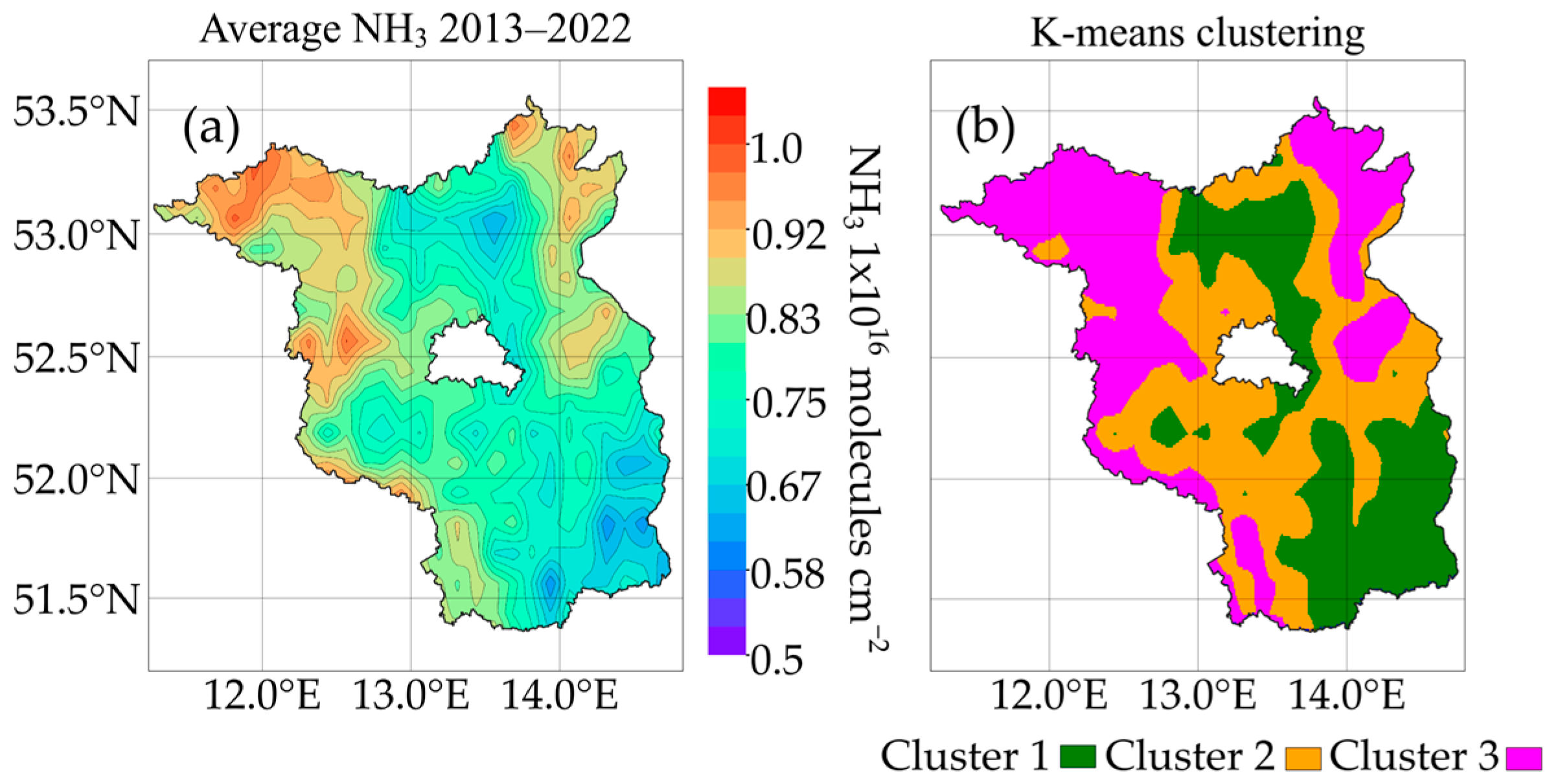
2.4. K-Means Clustering of NH₃ Emission

Clustering is an unsupervised machine learning technique used to organize large datasets based on similarity, thereby simplifying the subsequent analyses [61,62]. Cluster analysis is particularly advantageous for applications where prior knowledge of data patterns is unavailable [63].

The k-means algorithm is a widely used and robust method for partitioning data into k-clusters by iteratively selecting cluster centers (centroids) [61]. This algorithm assumes that the number of clusters (k) is predetermined [63,64].

K-means relies on the squared Euclidean distance for its calculations [65]. The Euclidean distance measures the separation between two points in a Euclidean space, which can have any number of dimensions [66]. For two points, p and q, in a j-dimensional space, the Euclidean distance d(p,q) is defined as

$$d\left(p,q\right)\sqrt{(p_1-q_1}{)}^2+(p_1-q_1{)}^2+\dots +(p_j-q_j{)}^2$$

(1)

The k-means algorithm partitions a dataset into clusters (k) by minimizing the variance within each cluster [66]. The primary input is a set of samples $X=\left\{x^1,\dots {,x}^n\right\}$ with $X^m=\left\{x_1^m,x_2^m,\dots ,x_j^m\right\}$ and m $ϵ$ $X=\left\{1,\dots ,n\right\}$ where n is the number of data points, and j is the number of variables. The $X$ sample is grouped for the k cluster subclasses $\left(S_1,S_2,\dots S_k\right)$ by reducing the total variance within each cluster $\left(S_{i=1,\dots ,k}\right)$, as shown in Equation (2):

$$\stackrel{\arg min}{S}\sum _{i=1}^k\sum _{X\in S_i}{‖X-{\mu }_i‖}^2$$

(2)

The term $‖X-{\mu }_i‖$ denotes the squared Euclidean distance between each sample ($X$) and its corresponding centroid (${\mu }_i$) in a dimensional Euclidean space [66]. In this study, k-means clustering was applied to analyze spatiotemporal NH₃ emissions over the aforementioned period [67,68]. The optimal number of clusters (k) was determined using the elbow method [69], which evaluates the Cluster Sum of Squares (CSS) to identify the point at which adding more clusters provides diminishing returns [66,70]. As shown in Supplementary Materials, Figure S2, the CSS curve exhibits an elbow at k = 3, indicating that this number of clusters offers a balance between minimizing the intra-cluster variance and maintaining interpretability. To further validate this choice, the Silhouette Score was computed, which measures cluster cohesion and separation [71,72,73]. The result confirmed that k = 3 provides an optimal balance between cluster compactness and separation compared to other values of k (Supplementary Materials Figure S3). Based on this, the dataset was divided into three clusters according to the emission levels. Furthermore, the clustering results were compared with NH₃ emission values and land cover types to determine the areas with significant emissions. This approach enabled the identification of high-emission regions, facilitating targeted environmental management and monitoring efforts.

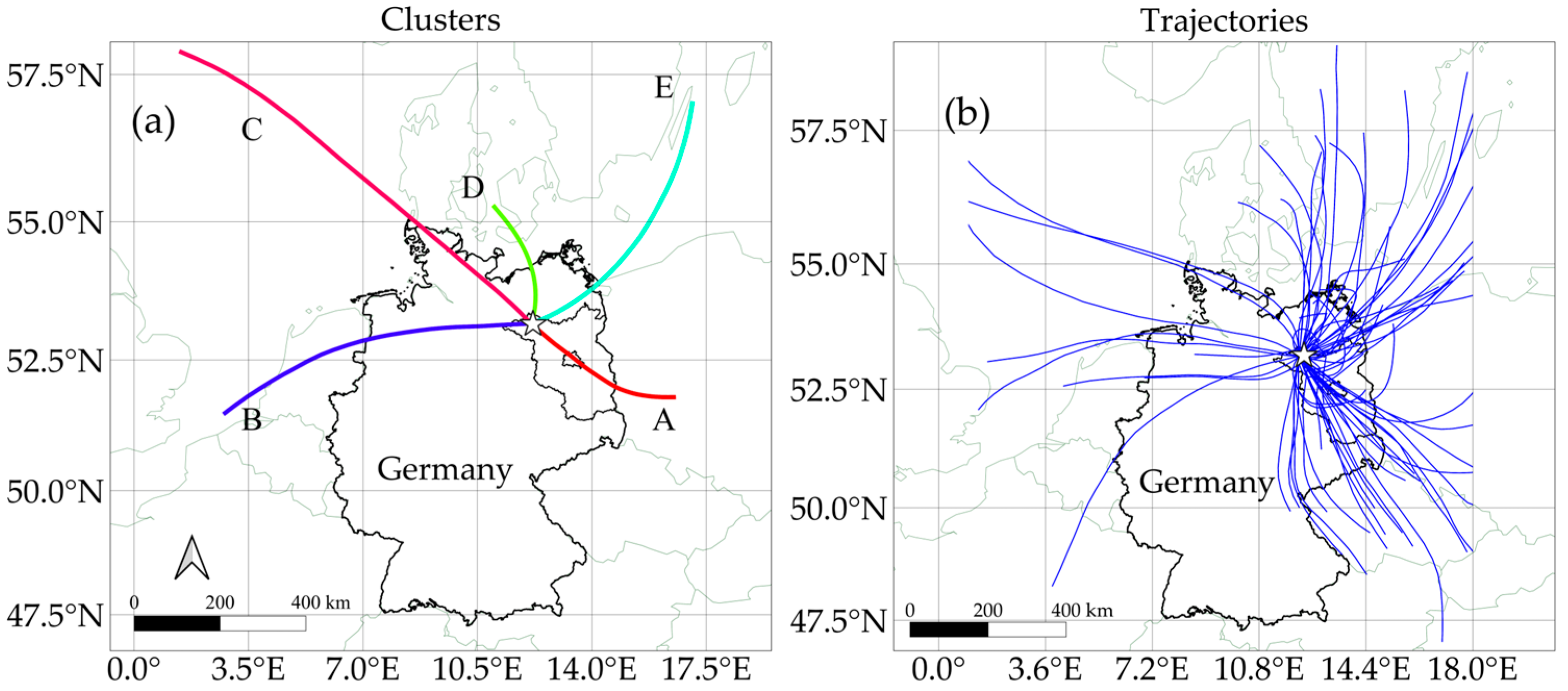
2.5. Back-Trajectories Analysis

The Hybrid Single-Particle Lagrangian Integrated Trajectory (HYSPLIT) atmospheric transport and dispersion model [74,75,76], developed by the National Oceanic and Atmospheric Administration (NOAA) Air Resources Laboratory (ARL), was employed for the backward trajectory analysis. HYSPLIT is widely employed in atmospheric transport and dispersion research, especially for determining long-range source-receptor connections. It has been applied in diverse research areas and contexts, including wildfire smoke dispersion [77], wind-blown dust transport [78] and volcanic ash dispersion [79]. Backward trajectories are particularly effective for identifying potential regional emission sources and clarifying the transport pathways.

In this study, backward trajectories were simulated at altitudes ranging from 500 to 1000 m above ground level (a.g.l.), using Global Data Assimilation System (GDAS1) meteorological data. The simulation was initiated at 00 UTC in March 2022, with a duration of 24 h. This altitude range provides sufficient insight into potential regional emission sources and transport pathways, while minimizing uncertainty. The analysis period was divided into five weeks: Week 1 (1–7 March), Week 2 (8–14 March), Week 3 (15–21 March), Week 4 (22–28 March), and Week 5 (29–31 March). These intervals were chosen based on the following criteria: (i) agricultural activities in spring and (ii) meteorological conditions, such as moderate temperature and variable humidity associated with transitional weather patterns [75], which influence atmospheric dispersion and pollutant concentrations. This approach enabled the identification of regions with elevated NH₃ emissions, providing valuable insights into environmental management and policy development.

3. Results

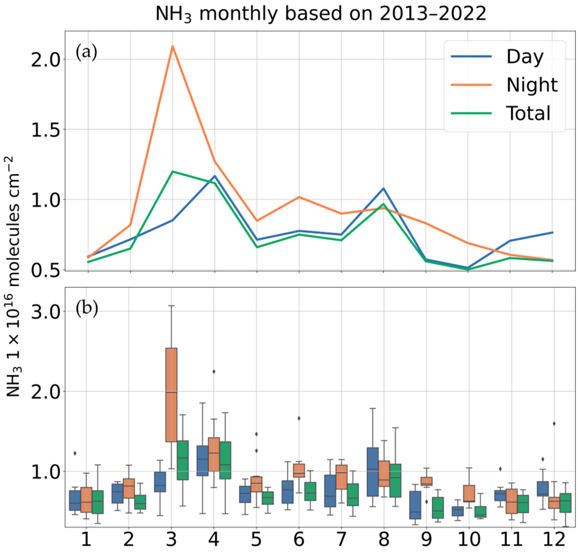
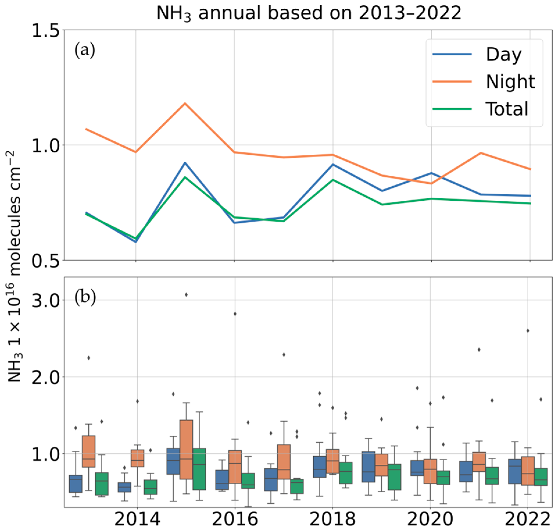
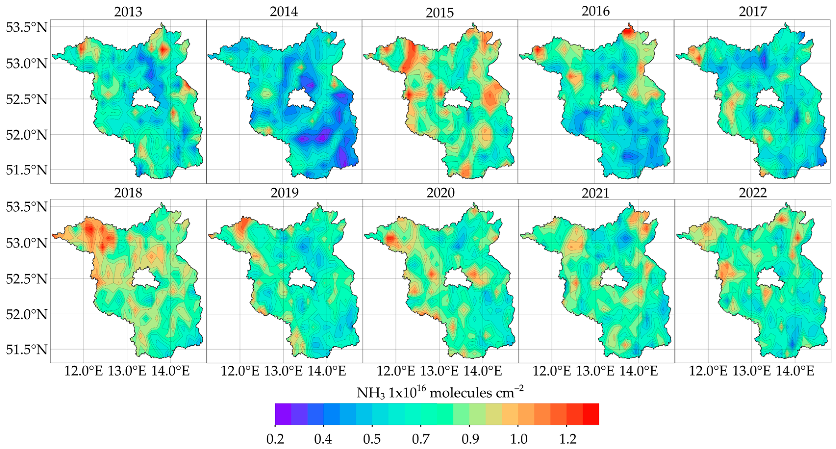
3.1. Spatiotemporal Variations of Ammonia Emissions

The spatial distribution of NH₃ emissions over Brandenburg across different periods (day, night, and total) allows for a comprehensive understanding of the diurnal variations in ammonia emissions. Morning overpasses capture daytime activities and emissions processes, whereas night overpasses reflect nighttime conditions. The total average integrates day and night observations, offering a complete representation of the ammonia levels in the atmosphere.

The climatological monthly average time series of NH₃ emissions from IASI-B illustrates significant temporal variability. Figure 2a highlights prominent peak concentrations for the total average period in March (1.2 × 10¹⁶ molecules cm⁻²), April (1.1 × 10¹⁶ molecules cm⁻²), and August (9.6 × 10¹⁵ molecules cm⁻²); conversely, the months with the lowest concentrations were observed in September (0.6 × 10¹⁵ molecules cm⁻²) and October (0.5 × 10¹⁵ molecules cm⁻²). The nighttime measurements exhibit a pronounced peak in March, exceeding 2.0 × 10¹⁶ molecules cm⁻².

As illustrated in Figure 2b, the annual NH₃ averages were observed in March (1.1 × 10¹⁶ molecules cm⁻² ± 4.0 × 10¹⁵ molecules cm⁻²) and April (1.1 × 10¹⁶ molecules cm⁻² ± 3.7 × 10¹⁵ molecules cm⁻²). These values decreased in May (6.6 × 10¹⁵ molecules cm⁻² ± 1.1 × 10¹⁵ molecules cm⁻²) but increased again in August (9.6 × 10¹⁵ molecules cm⁻² ± 3.5 × 10¹⁵ molecules cm⁻²).

Figure 3 presents the corresponding spatial distribution of climatological monthly average NH₃ emissions (×10 molecules cm⁻²) over Brandenburg. The map shows significant seasonal variations in NH₃ concentrations. During January and February, emissions were generally low and uniformly distributed. March and April exhibited notable increases, particularly in the northeastern region (around 53.2° N, 14.0° E) and northwestern (around 52.8° N, 11.9° E), likely due to agricultural activities such as fertilization. Emissions decreased slightly in May and June but remained elevated, with hotspots persisting in the northeastern area.

From July to September, NH₃ emissions were moderated, peaking again in August—possibly linked to post-harvest activities, and the emissions were mainly concentrated in the northeastern and northwestern regions. From October to December, the concentrations gradually declined, reaching their lowest values in December, with a relatively uniform distribution. Throughout the year, Brandenburg’s northeastern and northwestern regions consistently revealed higher NH₃ concentrations, indicating a persistent hotspot influenced by agricultural practices.

The annual time series of total NH₃ emissions displayed an oscillating pattern, with peak years in 2015 and 2018, followed by generally higher values from 2019 onward, as shown in Figure 4a. This trend was also evident in morning measurements, while nighttime concentrations showed more pronounced increases. Notably, clear peaks occurred in 2015 (1.3 × 10¹⁶ molecules cm⁻²) and 2022 (0.9 × 10¹⁵ molecules cm⁻²) could be observed.

The boxplot in Figure 4b shows the average NH₃ concentration distribution over the study period in Brandenburg, highlighting the variability across different years, with total concentrations in 2015 (8.6 × 10¹⁵ molecules cm⁻² ± 3.6 × 10¹⁵ molecules cm⁻²), 2018 (8.5 × 10¹⁵ molecules cm⁻² ± 3.3 × 10¹⁵ molecules cm⁻²), and 2022 (7.5 × 10¹⁵ molecules cm⁻² ± 3.5 × 10¹⁵ molecules cm⁻²⁾. Episodic events led to higher-than-average emissions during nighttime, while morning and total measurements indicated stable concentrations.

Figure 5 shows the spatial distribution of total NH₃ emissions, revealing distinct emission hotspots. The highest concentrations in 2015 were observed in the northwestern region (52.8° N to 53.3° N and 12.0° E to 12.5° E). This region consistently displays elevated NH₃ levels, making it a notable hotspot for several years. In addition to 2015, other years, such as 2013, 2018, and 2020, showed relatively high concentrations in the northwestern region of the country. The maps indicate a general trend of higher emissions in the northwestern region, while other areas exhibit moderate concentrations. In contrast, the southeastern part of Brandenburg (around 51.5° N to 52.5° N and 13.5° E to 14.8° E) showed a noticeable reduction in NH₃ concentrations from 2015 to 2022. This suggests a decrease in emissions or effective mitigation measures in this region over time.

Brandenburg’s strong seasonal variations influence NH₃ emissions, as illustrated in Figure 6. The boxplot categorizes the total column NH₃ emissions by season: winter, spring, summer, and autumn. The highest NH₃ emissions are observed in spring, with values reaching 1.8 × 10¹⁶ molecules cm⁻². This is likely due to increased agricultural activities, such as fertilization, during this season. Summer shows moderate emissions with a lower range of variability, while winter and autumn present the lowest NH₃ emissions, with autumn showing the least variation and the lowest overall emissions. The presence of outliers in summer suggests episodic high-emission events, possibly linked to specific agricultural practices and meteorological conditions.

Figure 7 provides the spatial distribution of NH₃ emissions for each season. In winter, emissions are uniformly low across the region. Spring shows significant hotspots, particularly in the northeastern and western parts of Brandenburg, indicating intense agricultural activity. Summer emissions are more evenly spread with some localized hotspots. In contrast, autumn sees a decrease in NH₃ levels, with a more uniform distribution resembling winter patterns. The northeastern and northwestern regions remain consistent NH₃ hotspots across all seasons, highlighting the strong influence of seasonal agricultural practices.

3.2. Meteorological Parameters and NH₃

Spatiotemporal NH₃ distributions are also dependent on meteorological conditions such as stability, circulation, temperature, and humidity [80,81]. The correlation matrix in Figure 8 illustrates the relationships between NH₃ concentrations and meteorological parameters from CAMS EAC4 data [58,59] based on their respective averages over the period 2013–2022 across the study area. The shape of the ellipse and the intensity of the color represent the strength and direction of the correlations, respectively. The color intensity also reflects the correlation magnitude: red shades represent positive correlations, while blue shades denote negative correlations. Numeric values within each cell quantify the correlation coefficient between pairs of variables. Positive values indicate a direct relationship, while negative values indicate an inverse relationship.

The observed positive matrix correlation between average NH₃ concentration and meteorological parameters averaged over time and across the defined study area, such as solar radiation (ssr) (r = 32), boundary layer height (blh) (r = 25), moisture flux (ie) (r = 21), temperature at 2 m (t2m) (r = 11), and convective available potential energy (cape) (r = 5). This suggests that these factors enhance NH₃ volatilization, particularly in agricultural areas, by promoting favorable conditions for its release. Conversely, NH₃ concentrations were negatively correlated with wind speed (wind spd.) (r = −17), evaporation (e) (r = −19), and total precipitation (tp) (r = −26) imply that these conditions could lead to reduced NH₃ values, potentially due to dilution, dispersion, or removal through the deposition process.

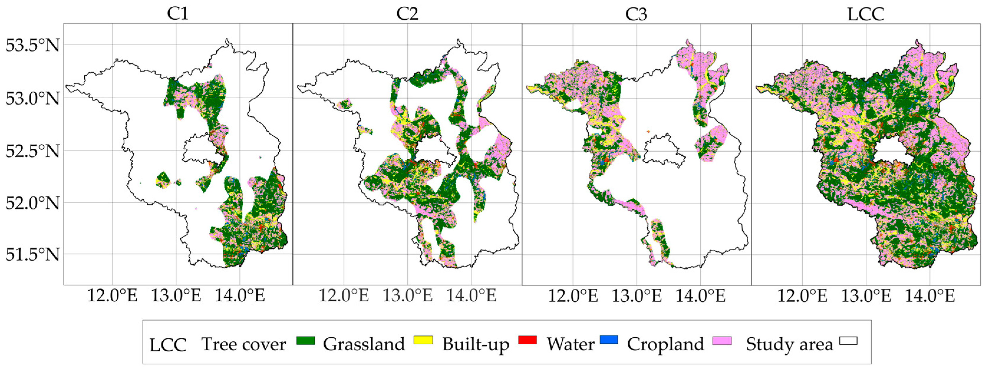
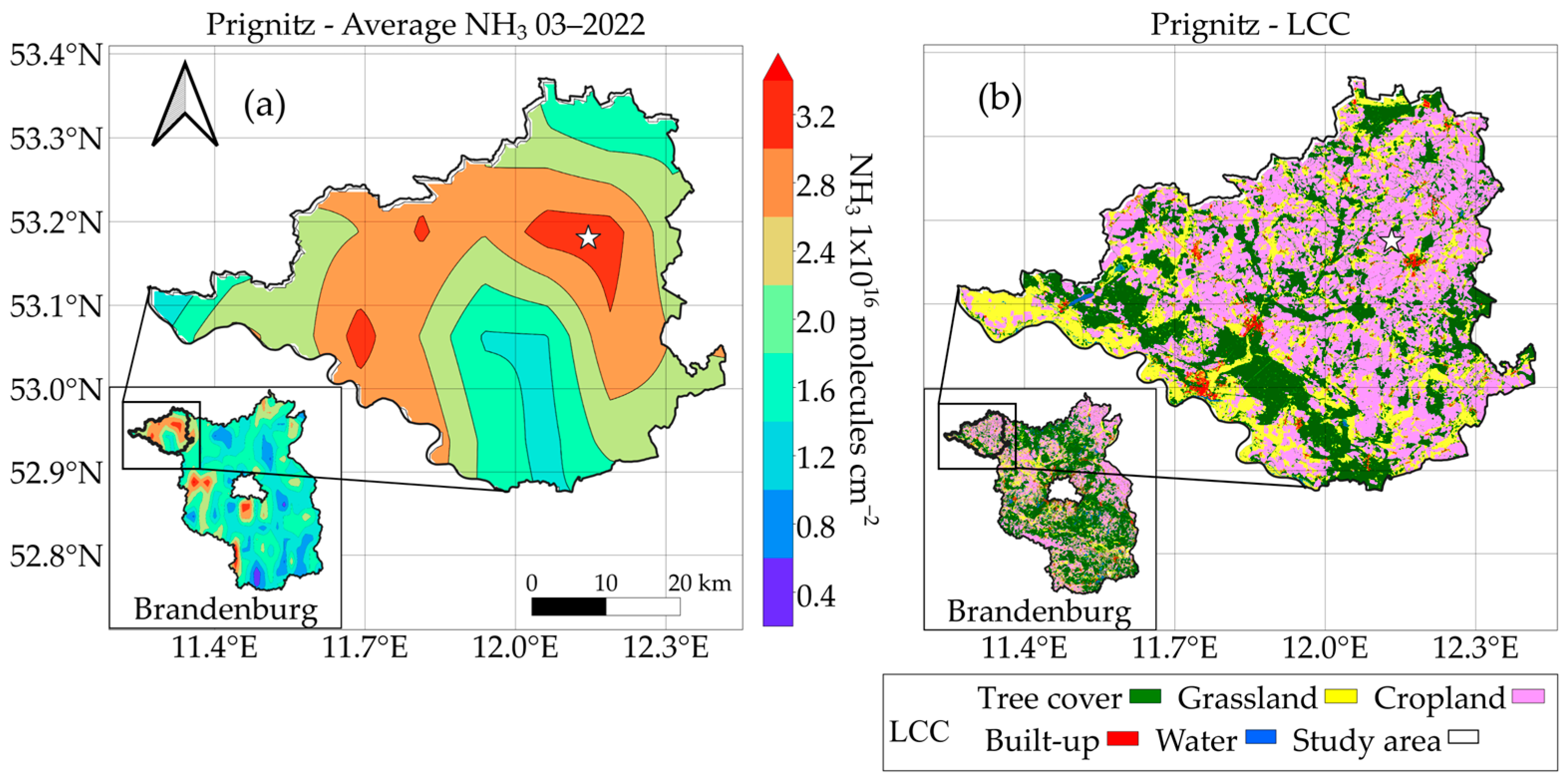
3.3. Land-Use-Related NH₃ Emissions

To identify land-use-related NH₃ emissions, a k-means cluster analysis was conducted, partitioning regions of varying NH₃ concentrations into three distinct clusters: Cluster 1, Cluster 2, and Cluster 3. Figure 9 shows the time series monthly average over Brandenburg, where Cluster 1 represents the lowest concentration (0.5 × 10¹⁵ molecules cm⁻² to 0.7 × 10¹⁵ molecules cm⁻²), Cluster 2 represents the moderated concentration (0.7 × 10¹⁵ molecules cm⁻² to 0.8 × 10¹⁵ molecules cm⁻²), and Cluster 3 represents the highest concentration (0.9 × 10¹⁵ molecules cm⁻² to 1.1 × 10¹⁶ molecules cm⁻²). These values are mapped to the sequential position of spatial data pixels, reflecting the spatial distribution of NH₃ concentrations across the region. The pixel index corresponds to specific geographic locations. Cluster 2 has the highest number of pixel indices, exceeding 250, followed by Cluster 1 with over 150 pixel indices, and finally, Cluster 3 with approximately 200 pixel indices.

The spatial distribution (Figure 10a) reveals that higher NH₃ concentrations are predominantly found in the northwest to central regions, while the southern regions exhibit lower concentrations. Cluster 3, associated with built-up areas and croplands, displays the highest NH₃ emissions, particularly in urban centers and intensive agricultural zones, indicating that anthropogenic activities such as vehicular traffic and fertilizer application are significant contributors. Figure 10b further refines these findings through spatial clustering, showing that agricultural zones in the northeast and northwest exhibit the highest NH₃ concentrations, whereas lower emissions are found in forested and non-agricultural areas in the north-central and southern regions.

Masking the LCC with the three clusters (Figure 11) displays the respective areas. Cluster 1 predominantly comprises regions characterized by tree cover, grasslands, and water bodies, where NH₃ emissions are relatively low. This suggests that natural landscapes with significant vegetation cover tend to act as NH₃ sinks, reducing emissions. These areas are dispersed across Brandenburg, including natural reserves and forested regions. Cluster 2 covers regions with mixed land cover types, including grassland and cropland. The NH₃ emissions in this cluster are moderate, reflecting the mixed influence of natural and anthropogenic sources. The spatial distribution indicates that areas with diverse land cover types experience varying degrees of agricultural activities, which are a significant contributor but are moderated by the presence of natural vegetation.

Cluster 3, with the highest emissions, is primarily dominated by croplands (8%), further reinforcing the association between agricultural land use and NH₃ emissions. This suggests that anthropogenic activities, such as vehicular traffic and fertilizer application, are major contributors to NH₃ pollution. The central part of the study region, including areas surrounding Berlin to the east and west, falls within this cluster, emphasizing the influence of urbanization and agricultural intensification.

The total land area distribution of Brandenburg (

Table 1. Land cover composition (percentage and area) for three clusters over Brandenburg.

	Cluster 1		Cluster 2		Cluster 3
LCC	Percentage %	Area km2	Percentage %	Area km2	Percentage %	Area km2
Tree Cover	13.11	4531.837	22.55	5544.947	5.86	3060.388
Grassland	4.71	1631	10.17	2237.918	3.93	2047.746
Cropland	5.1	1760.729	15.55	3050.081	8.02	4172.607
Built-up	0.81	282.08	1.44	357.85	0.38	197.77
Water	0.77	265.98	1.34	317.758	0.36	187.211

) shows that Cluster 2 covers the largest proportion of Brandenburg (11,508.5 km², 51.05%), followed by Cluster 1 (8471.62 km², 24.5%), and Cluster 3 (9665.72 km², 18.55%). This spatial partitioning highlights the strong influence of land cover on NH₃ emissions, with agricultural land use being the dominant source of NH₃ emissions in the study area.

3.4. Case Study of NH₃ Emission Using HYSPLIT

To further investigate the origin of NH₃ emissions (i.e., local versus non-local sources), a case study was conducted using the HYSPLIT trajectory model. This analysis focused on hotspot areas identified using the NH₃ concentration data. March was selected as the study period because it marks the transition from winter to spring, coinciding with the onset of agricultural activities that are major contributors to NH₃ emissions. Figure 12a illustrates the NH₃ concentration levels across Brandenburg, highlighting the significant spatial variability and particularly high values in the northwest subregion. Reaching levels of approximately 3.2 × 10¹⁶ molecules cm⁻². The northwestern region of the study site emerged as an agricultural hotspot driving NH₃ emissions during peak periods, such as March.

The highest NH₃ emission values in the northeast were associated with intense agricultural activities, including cattle and fruit farming, and the proximity of two local airfields. This hotspot corresponded to major agricultural zones, as classified under Cluster 3 in Figure 12b.

Table 2. Land cover composition (percentage and area) related to the cluster over northwestern subregion.

LCC	%	km2
Tree Cover	14.62	621.47235
Grassland	11.34	481.81842
Cropland	22.11	938.78178
Built-up	0.8	34.07092
Water	0.33	13.84679

shows the distribution of the different LCCs across the subregion. Cropland is predominantly present (22.11%), indicating a significant agriculture zone, followed by tree cover (14.62%) and grassland (11.34%).

To assess the potential source regions influencing NH₃ levels, HYSPLIT backward trajectories were grouped into five clusters (A–E), as presented in

Table 3. Cluster dispersion trajectories (percentage and direction) over the northwestern subregion.

Cluster	Frequency	Direction
A	20	SE
B	5	W
C	18	NW
D	32	N
E	25	NEN

, along with their frequency percentages and directions. These clusters represent distinct air mass sectors affecting the region and highlight the exposure of the lowlands to both local and regional air masses.

The clusters categorized into long-, medium-, and short-range transport are shown in Figure 13a, providing a detailed view of the trajectories for each cluster at an arrival height ranging from 500–1000 m a.g.l. During the study period. Cluster D, originating from the north, is the most frequent, accounting for 32% of the total trajectories, indicating that northern air masses play a dominant role in shaping the region’s atmospheric conditions. This cluster represents slow-moving air masses and illustrates the contribution of relatively local sources to NH₃ emissions. Cluster E, with a northeast to east-north-east (NEN) origin, is the second most prevalent, contributing 25% of the trajectories, likely influenced by airflows from northern Poland or the Baltic Sea region. Cluster A, originating from the southeast, accounts for 20%, reflecting the influence of air masses from central or eastern Europe. Cluster C, representing 18% of the trajectories, originates from the northwest, suggesting the potential impact of maritime air from the North Sea and surrounding regions. These air masses can carry emissions over long distances before reaching the northwestern subregion. Furthermore, Cluster B, with its origin in the North Sea, has the lowest frequency at 5%, indicating occasional airflows from industrialized regions in western Germany or the Netherlands. The results highlight that trajectories from the north (Cluster D, 32%), northeast (25%), and northwest (18%) account for 75% of the air masses contributing to the NH₃ concentrations.

4. Discussion

The use of thermal infrared wavelengths by IASI-B has significantly enhanced our ability to detect NH₃ over broad spatial scales compared to ground-based monitoring networks. Recent studies, such as that by Coheur P. et al. [21], used IASI to evaluate NH₃ emissions and assess the influence of local sources, particularly agricultural activities. Van Damme et al. [7] introduced an advanced retrieval method for NH₃ using IASI based on the computation of a dimensionless metric known as the Hyperspectral Range Index (HRI). Subsequent research by [82] demonstrated the effectiveness of these retrievals, although significant variability in the measurement uncertainty was noted. In this study, the spatiotemporal variation of NH₃ emission was analyzed over eastern German lowlands using the IASI-B sensor from the satellite MetOp-B [36,50,51,52]. This analysis encompassed various aggregation periods, including climatological monthly, annual, and seasonal patterns observed during different satellite overpasses. The results (Figure 2 and Figure 3) show that NH₃ emissions peaked in March (1.2 × 10¹⁶ molecules cm⁻²) and April (1.1 × 10¹⁶ molecules cm⁻²). This seasonal peak coincides with the European spring fertilization period, a pattern consistent with previous studies by Abeed R. et al. [26]. Early fertilization practices during this period are likely to contribute factors to the observed NH₃ peaks. Additionally, observation of the IASI dataset of the average NH₃ timeseries reported by Van Dame et al. [36] corroborates these findings, indicating that NH₃ concentrations typically rise during the principal fertilization periods in Europe (March-April and July-August). In contrast, emissions were lowest during autumn and winter, with the lowest in September (0.6× 10¹⁵ molecules cm⁻²) (Figure 2). This is consistent with the findings of Kuhn T. [83], who noted that fertilizer applications in Germany are regulated during these seasons, leading to decreased emissions.

This study identified significant interannual variability in NH₃ emissions (Figure 5), with notable peaks in 2015, 2018, 2019, and 2022. Spatial analysis revealed that the northwestern region of Brandenburg consistently exhibited higher NH₃ emissions than the other regions. This region has been impacted by wildfires during periods of drought and dryness in recent years, coinciding with the years of peak NH₃ emissions. Supporting evidence from [84] indicates that Brandenburg experienced the highest number of forest fires in Germany between 2002 and 2022, with significant contributions from heatwaves in 2018 and 2019, as also demonstrated by [45]. Additional sources of elevated NH₃ emissions include anthropogenic activities near transportation hubs, such as Berlin Brandenburg Airport (opened in 2020), which may have contributed to the region’s NH₃ footprint.

Distinct diurnal patterns of NH₃ concentrations were observed, with nighttime levels consistently higher than daytime levels [84] emphasized that daytime satellite observations are more reliable due to improved atmospheric mixing and dispersion, which reduces localized emission effects. Conversely, nighttime observations are subject to greater relative errors due to lower thermal contrast, as reported by Van Damme et al. [84]. Thermal inversions, as demonstrated by [25,55], may confine NH₃ within the boundary layer at night, further contributing to the elevated concentrations.

Meteorological factors clearly affect NH₃ emissions. The correlation matrix illustrated a negative correlation between NH₃ concentrations and wind speed (r = −17), evaporation (r = −19), and total precipitation (r = −26), suggesting that these factors disperse NH₃ concentrations, as confirmed by [85]. In contrast, positive correlations with air temperature (r = 11) and solar radiation (r = 32) suggest that warmer conditions and increased solar energy enhance NH₃ volatilization, particularly in agricultural areas. These findings are consistent with those of [81,86]. Furthermore, wind direction plays a critical role, as highlighted by [87,88].

Land cover type significantly influences NH₃ emissions, as shown in this study (Figure 11). A 10-year analysis revealed hotspots in Brandenburg, primarily in agricultural regions in the northeast, northwest, and western regions. Spatial k-means partitioning clustering identified three distinct emission patterns: Cluster 3, with the highest NH₃ concentration, predominantly covered croplands and accounted for 8% of the total area (9665.722 km²). In contrast, clusters 1 and 2 exhibited lower and moderate NH₃ concentrations, covering 15% of the total area (11,508.554 km²) and 5% (8471.626 km²), respectively. This indicates that agricultural land use types are likely significant contributors to NH₃ emissions, which is consistent with the findings of previous studies [12,50,54,89]. The authors identified agricultural practices as the primary source of NH₃ emissions, contributing to over 80% of the total NH₃ in Europe [26].

HYSPLIT backward trajectory analysis for March 2022 as a case study further highlighted the influence of local and non-local contributions. Trajectories from the north (D, 32%), northeast (E, 25%), and northwest (C, 18%) accounted for 75% of the air mass contributing to the NH₃ concentrations. However, [90,91] emphasized that the accuracy of a single trajectory is constrained by several uncertainties, including meteorological inputs, which only provide an approximation of air mass pathways. The northwestern region of the study site emerged as an agricultural hotspot driving NH₃ emissions during peak periods, such as March.

Finally, our study comprehensively examined the spatiotemporal variations in NH₃ derived from IASI-B, analyzing the underlying factors that contribute to the current pattern. It provides an overview of NH₃ emissions over the past ten years. It is worth noting that the peaks of NH₃ occurring during March and August in this study closely correspond to those in previous studies. These peaks coincide with agricultural practices, such as fertilizer use and the growing season, suggesting a direct link between LCC and emission patterns. Additionally, climate change is likely to exacerbate NH₃ emissions by increasing the frequency of conditions that enhance NH₃ concentrations, such as high temperatures and droughts. This underscores the importance of continuous monitoring and further research on the effects of changing climate patterns on NH₃ emissions. In addition to agricultural activities, the detection of hotspots suggests that transportation hubs and industrial activities could also be significant contributors to NH₃ emissions. Additionally, wildfires—particularly in recent years—have contributed to increased emissions.

5. Conclusions

NH₃ emission plays a critical role in air quality and ecosystem health. This study comprehensively analyzed the spatiotemporal variations in NH₃ emissions in the eastern German lowlands over 10 years using IASI-B satellite data. By combining satellite-based clustering analysis and trajectory modeling, key emission patterns, dominant hotspots, and meteorological influences were identified. The findings demonstrated distinct diurnal and seasonal NH₃ patterns, with morning emissions remaining stable and nighttime hours showing higher concentrations, likely due to reduced atmospheric mixing. Seasonally, NH₃ emissions peaked in the months of March, April, and August, with concentrations reaching up to 3.2 × 10¹⁶ molecules cm⁻², particularly in hotspot areas. These peaks correspond to spring fertilization and summer post-harvest emissions, particularly in cropland-dominated areas. K-means clustering analysis confirmed that Cluster 3 (croplands and urban areas) exhibited the highest NH₃ emissions, covering 18.55% of the total area (9665.72 km²), where 8% of this area corresponds to croplands, while Cluster 1 (forested region) had the lowest emissions, covering 24.5% of the total area (8471.62 km²).

Meteorological conditions also play a crucial role in influencing the NH₃ emissions. The analysis revealed a negative correlation between NH₃ concentrations and precipitation (pt) (r = −26), wind speed (wind spd.) (r = −17), and evaporation (e) (r = −19), indicating that weather conditions substantially affect the dispersion of NH₃ emissions. In contrast, higher temperatures (t2m), solar radiation (ssr), and boundary layer height (blh) (correlations of r = 11, r = 32, and r = 25, respectively) were associated with increased NH₃ volatilization. Additionally, the findings underscore the importance of considering other potential contributors, such as wildfires or agricultural fires, which may further impact NH₃ emissions in agricultural regions.

HYSPLIT back-trajectory analysis revealed that local agricultural activities are the main contributors to NH₃ emissions, particularly during peak farming periods. A case study conducted in March 2022 demonstrated that agricultural practices and other anthropogenic sources, such as local airfields, significantly increased NH₃ levels. Air masses from the north (Cluster D: 32%) and northeast (Cluster E: 25%) carried significant NH₃ loads, emphasizing the regional-scale transport mechanisms. Additional sources, such as local airfields and wildfires, also contributed to episodic emission spikes.

These findings underscore the necessity for improved NH₃ emission monitoring, particularly in agricultural regions that are vulnerable to climate change. The integration of satellite-based and ground-based observations can enhance mitigation strategies, and support climate-smart agricultural practices. Future research should focus on improving emission inventories, assessing long-term trends under changing climatic conditions, exploring how NH₃ emissions contribute to PM_2.5, and exploring additional anthropogenic NH₃ contributions, such as transportation and industrial activities.

References

1. Zhou, C.; Zhou, H.; Holsen, T.M.; Hopke, P.K.; Edgerton, E.S.; Schwab, J.J. Ambient Ammonia Concentrations Across New York State. J. Geophys. Res. Atmos. 2019, 124, 8287–8302. [Google Scholar] [CrossRef]
2. Acharja, P.; Ali, K.; Ghude, S.D.; Sinha, V.; Sinha, B.; Kulkarni, R.; Gultepe, I.; Rajeevan, M.N. Enhanced Secondary Aerosol Formation Driven by Excess Ammonia during Fog Episodes in Delhi, India. Chemosphere 2022, 289, 133155. [Google Scholar] [CrossRef] [PubMed]
3. Farren, N.J.; Davison, J.; Rose, R.A.; Wagner, R.L.; Carslaw, D.C. Underestimated Ammonia Emissions from Road Vehicles. Environ. Sci. Technol. 2020, 54, 15689–15697. [Google Scholar] [CrossRef] [PubMed]
4. Wang, S.; Nan, J.; Shi, C.; Fu, Q.; Gao, S.; Wang, D.; Cui, H.; Saiz-Lopez, A.; Zhou, B. Atmospheric Ammonia and Its Impacts on Regional Air Quality over the Megacity of Shanghai, China. Sci. Rep. 2015, 5, 15842. [Google Scholar] [CrossRef]
5. Van Damme, M.; Clarisse, L.; Franco, B.; Sutton, M.A.; Erisman, J.W.; Wichink Kruit, R.; van Zanten, M.; Whitburn, S.; Hadji-Lazaro, J.; Hurtmans, D.; et al. Global, Regional and National Trends of Atmospheric Ammonia Derived from a Decadal (2008–2018) Satellite Record. Environ. Res. Lett. 2021, 16, 055017. [Google Scholar] [CrossRef]
6. Jalali, S.; Karbakhsh, M.; Momeni, M.; Taheri, M.; Amini, S.; Mansourian, M.; Sarrafzadegan, N. Long-Term Exposure to PM2.5 and Cardiovascular Disease Incidence and Mortality in an Eastern Mediterranean Country: Findings Based on a 15-Year Cohort Study. Environ. Health 2021, 20, 112. [Google Scholar] [CrossRef]
7. Van Damme, M.; Erisman, J.W.; Clarisse, L.; Dammers, E.; Whitburn, S.; Clerbaux, C.; Dolman, A.J.; Coheur, P.-F. Worldwide Spatiotemporal Atmospheric Ammonia (NH3) Columns Variability Revealed by Satellite. Geophys. Res. Lett. 2015, 42, 8660–8668. [Google Scholar] [CrossRef]
8. Sutton, M.A.; Reis, S.; Riddick, S.N.; Dragosits, U.; Nemitz, E.; Theobald, M.R.; Tang, Y.S.; Braban, C.F.; Vieno, M.; Dore, A.J.; et al. Towards a Climate-Dependent Paradigm of Ammonia Emission and Deposition. Philos. Trans. R. Soc. B Biol. Sci. 2013, 368, 20130166. [Google Scholar] [CrossRef]
9. Dammers, E.; Palm, M.; Van Damme, M.; Vigouroux, C.; Smale, D.; Conway, S.; Toon, G.C.; Jones, N.; Nussbaumer, E.; Warneke, T.; et al. An Evaluation of IASI-NH3 with Ground-Based Fourier Transform Infrared Spectroscopy Measurements. Atmos. Chem. Phys. 2016, 16, 10351–10368. [Google Scholar] [CrossRef]
10. Herrera, B.; Bezanilla, A.; Blumenstock, T.; Dammers, E.; Hase, F.; Clarisse, L.; Magaldi, A.; Rivera, C.; Stremme, W.; Strong, K.; et al. Measurement Report: Evolution and Distribution of NH3 over Mexico City from Ground-Based and Satellite Infrared Spectroscopic Measurements. Atmos. Chem. Phys. 2022, 22, 14119–14132. [Google Scholar] [CrossRef]
11. Sutton, M.A.; Nemitz, E.; Erisman, J.W.; Beier, C.; Bahl, K.B.; Cellier, P.; de Vries, W.; Cotrufo, F.; Skiba, U.; Di Marco, C.; et al. Challenges in Quantifying Biosphere–Atmosphere Exchange of Nitrogen Species. Environ. Pollut. 2007, 150, 125–139. [Google Scholar] [CrossRef]
12. Gu, B.; Sutton, M.A.; Chang, S.X.; Ge, Y.; Chang, J. Agricultural Ammonia Emissions Contribute to China’s Urban Air Pollution. Front. Ecol. Environ. 2014, 12, 265–266. [Google Scholar] [CrossRef]
13. Nowak, J.B.; Neuman, J.A.; Bahreini, R.; Brock, C.A.; Middlebrook, A.M.; Wollny, A.G.; Holloway, J.S.; Peischl, J.; Ryerson, T.B.; Fehsenfeld, F.C. Airborne Observations of Ammonia and Ammonium Nitrate Formation over Houston, Texas. J. Geophys. Res. 2010, 115, D22304. [Google Scholar] [CrossRef]
14. Liu, Z.; Rieder, H.E.; Schmidt, C.; Mayer, M.; Guo, Y.; Winiwarter, W.; Zhang, L. Optimal Reactive Nitrogen Control Pathways Identified for Cost-Effective PM2.5 Mitigation in Europe. Nat. Commun. 2023, 14, 4246. [Google Scholar] [CrossRef] [PubMed]
15. Geng, G.; Xiao, Q.; Liu, S.; Liu, X.; Cheng, J.; Zheng, Y.; Xue, T.; Tong, D.; Zheng, B.; Peng, Y.; et al. Tracking Air Pollution in China: Near Real-Time PM5 Retrievals from Multisource Data Fusion. Environ. Sci. Technol. 2021, 55, 12106–12115. [Google Scholar] [CrossRef]
16. Jiang, F.; Chen, B.; Li, P.; Jiang, J.; Zhang, Q.; Wang, J.; Deng, J. Spatio-Temporal Evolution and Influencing Factors of Synergizing the Reduction of Pollution and Carbon Emissions—Utilizing Multi-Source Remote Sensing Data and GTWR Model. Environ. Res. 2023, 229, 115775. [Google Scholar] [CrossRef]
17. Bouwman, A.F.; Lee, D.S.; Asman, W.A.; Dentener, F.J.; Van Der Hoek, K.W.; Olivier, J.G.J. A Global High-resolution Emission Inventory for Ammonia. Glob. Biogeochem. Cycles 1997, 11, 561–587. [Google Scholar] [CrossRef]
18. Guo, X.; Wang, R.; Pan, D.; Zondlo, M.A.; Clarisse, L.; Van Damme, M.; Whitburn, S.; Coheur, P.; Clerbaux, C.; Franco, B.; et al. Validation of IASI Satellite Ammonia Observations at the Pixel Scale Using In Situ Vertical Profiles. J. Geophys. Res. Atmos. 2021, 126, e2020JD033475. [Google Scholar] [CrossRef]
19. Zhu, L.; Henze, D.K.; Bash, J.O.; Cady-Pereira, K.E.; Shephard, M.W.; Luo, M.; Capps, S.L. Sources and Impacts of Atmospheric NH3: Current Understanding and Frontiers for Modeling, Measurements, and Remote Sensing in North America. Curr. Pollut. Rep. 2015, 1, 95–116. [Google Scholar] [CrossRef]
20. Jacob, D.J.; Turner, A.J.; Maasakkers, J.D.; Sheng, J.; Sun, K.; Liu, X.; Chance, K.; Aben, I.; McKeever, J.; Frankenberg, C. Satellite Observations of Atmospheric Methane and Their Value for Quantifying Methane Emissions. Atmos. Chem. Phys. 2016, 16, 14371–14396. [Google Scholar] [CrossRef]
21. Coheur, P.-F.; Clarisse, L.; Turquety, S.; Hurtmans, D.; Clerbaux, C. IASI Measurements of Reactive Trace Species in Biomass Burning Plumes. Atmos. Chem. Phys. 2009, 9, 5655–5667. [Google Scholar] [CrossRef]
22. Clarisse, L.; Clerbaux, C.; Dentener, F.; Hurtmans, D.; Coheur, P.-F. Global Ammonia Distribution Derived from Infrared Satellite Observations. Nat. Geosci. 2009, 2, 479–483. [Google Scholar] [CrossRef]
23. Van Damme, M.; Clarisse, L.; Whitburn, S.; Hadji-Lazaro, J.; Hurtmans, D.; Clerbaux, C.; Coheur, P.-F. Industrial and Agricultural Ammonia Point Sources Exposed. Nature 2018, 564, 99–103. [Google Scholar] [CrossRef] [PubMed]
24. Wagner, S.; Angenendt, E.; Beletskaya, O.; Zeddies, J. Assessing Ammonia Emission Abatement Measures in Agriculture: Farmers’ Costs and Society’s Benefits—A Case Study for Lower Saxony, Germany. Agric. Syst. 2017, 157, 70–80. [Google Scholar] [CrossRef]
25. Jacobsen, B.H.; Latacz-Lohmann, U.; Luesink, H.; Michels, R.; Ståhl, L. Costs of Regulating Ammonia Emissions from Livestock Farms near Natura 2000 Areas—Analyses of Case Farms from Germany, Netherlands and Denmark. J. Environ. Manag. 2019, 246, 897–908. [Google Scholar] [CrossRef]
26. Abeed, R.; Viatte, C.; Porter, W.C.; Evangeliou, N.; Clerbaux, C.; Clarisse, L.; Van Damme, M.; Coheur, P.-F.; Safieddine, S. Estimating Agricultural Ammonia Volatilization over Europe Using Satellite Observations and Simulation Data. EGUsphere 2022, 2022, 1–28. [Google Scholar] [CrossRef]
27. Pohl, V.; Gilmer, A.; Hellebust, S.; McGovern, E.; Cassidy, J.; Byers, V.; McGillicuddy, E.J.; Neeson, F.; O’Connor, D.J. Ammonia Cycling and Emerging Secondary Aerosols from Arable Agriculture: A European and Irish Perspective. Air 2022, 1, 37–54. [Google Scholar] [CrossRef]
28. Zhan, X.; Adalibieke, W.; Cui, X.; Winiwarter, W.; Reis, S.; Zhang, L.; Bai, Z.; Wang, Q.; Huang, W.; Zhou, F. Improved Estimates of Ammonia Emissions from Global Croplands. Environ. Sci. Technol. 2021, 55, 1329–1338. [Google Scholar] [CrossRef]
29. R’Honi, Y.; Clarisse, L.; Clerbaux, C.; Hurtmans, D.; Duflot, V.; Turquety, S.; Ngadi, Y.; Coheur, P.-F. Exceptional Emissions of NH3 and HCOOH in the 2010 Russian Wildfires. Atmos. Chem. Phys. 2013, 13, 4171–4181. [Google Scholar] [CrossRef]
30. Whitburn, S.; Van Damme, M.; Clarisse, L.; Hurtmans, D.; Clerbaux, C.; Coheur, P.-F. IASI-Derived NH3 Enhancement Ratios Relative to CO for the Tropical Biomass Burning Regions. Atmos. Chem. Phys. 2017, 17, 12239–12252. [Google Scholar] [CrossRef]
31. Malherbe, L.; German, R.; Couvidat, F.; Zanatta, L.; Blannin, L.; James, A.; Lètinois, L.; Schucht, S.; Berthelot, B.; Raoult, J. Emissions of Ammonia and Methane from the Agricultural Sector Emissions from Livestock Farming; ETC HE: Jülich, Germany, 2022; ISBN 978-82-93970-25-5. [Google Scholar]
32. European Union DIRECTIVE (EU) 2016/2284 OF THE EUROPEAN PARLIAMENT AND OF THE COUNCIL—Of 14 December 2016—On the Reduction of National Emissions of Certain Atmospheric Pollutants, Amending Directive 2003/35/EC and Repealing Directive 2001/81/EC. 2016. Available online: https://eur-lex.europa.eu/legal-content/EN/TXT/?uri=CELEX:32016L2284 (accessed on 5 June 2024).
33. UmweltBundesamt Ammoniak-Emissionen. 2016. Available online: https://www.umweltbundesamt.de/daten/luft/luftschadstoff-emissionen-in-deutschland/ammoniak-emissionen#entwicklung-seit-1990 (accessed on 27 June 2024).
34. Umweltbundesamt Background March 2023: Air Quality 2022 (Preliminary Evaluation). 2023. Available online: https://www.umweltbundesamt.de/sites/default/files/medien/479/publikationen/2023_uba_hgp_luftqualitaet_engl_bf.pdf (accessed on 6 May 2024).
35. Kleemola-Juntunen, P.; Kirchner, S. Gothenburg Protocol and Convention on Long-Range Transboundary Air Pollutions. In Global Encyclopedia of Territorial Rights; Springer International Publishing: Cham, Switzerland, 2021; pp. 1–8. [Google Scholar]
36. Van Damme, M.; Clarisse, L.; Stavrakou, T.; Wichink Kruit, R.; Sellekaerts, L.; Viatte, C.; Clerbaux, C.; Coheur, P.F. On the Weekly Cycle of Atmospheric Ammonia over European Agricultural Hotspots. Sci. Rep. 2022, 12, 12327. [Google Scholar] [CrossRef] [PubMed]
37. Clerbaux, C.; Boynard, A.; Clarisse, L.; George, M.; Hadji-Lazaro, J.; Herbin, H.; Hurtmans, D.; Pommier, M.; Razavi, A.; Turquety, S.; et al. Monitoring of Atmospheric Composition Using the Thermal Infrared IASI/MetOp Sounder. Atmos. Chem. Phys. 2009, 9, 6041–6054. [Google Scholar] [CrossRef]
38. Clarisse, L.; Franco, B.; Van Damme, M.; Gioacchino, T.D.; Hadji-Lazaro, J.; Whitburn, S.; Noppen, L.; Hurtmans, D.; Clerbaux, C.; Coheur, P. The IASI NH 3 Version 4 Product: Averaging Kernels and Improved Consistency. Atmos. Meas. Tech. Discuss. 2023, 2023, 1–31. [Google Scholar] [CrossRef]
39. Unger, M.; Lakes, T. Land Use Conflicts and Synergies on Agricultural Land in Brandenburg, Germany. Sustainability 2023, 15, 4546. [Google Scholar] [CrossRef]
40. Statistisches Jahrbuch 2020—Brandenburg Amt Für Statistik Berlin-Brandenburg; Amt Für Statistik Berlin-Brandenburg: Potsdam, Germany, 2020.
41. Reyer, C.; Bachinger, J.; Bloch, R.; Hattermann, F.F.; Ibisch, P.L.; Kreft, S.; Lasch, P.; Lucht, W.; Nowicki, C.; Spathelf, P.; et al. Climate Change Adaptation and Sustainable Regional Development: A Case Study for the Federal State of Brandenburg, Germany. Reg. Environ. Chang. 2012, 12, 523–542. [Google Scholar] [CrossRef]
42. Gutzler, C.; Helming, K.; Balla, D.; Dannowski, R.; Deumlich, D.; Glemnitz, M.; Knierim, A.; Mirschel, W.; Nendel, C.; Paul, C.; et al. Agricultural Land Use Changes—A Scenario-Based Sustainability Impact Assessment for Brandenburg, Germany. Ecol. Indic. 2015, 48, 505–517. [Google Scholar] [CrossRef]
43. Mirschel, W.; Wieland, R.; Luzi, K.; Groth, K. Model-Based Estimation of Irrigation Water Demand for Different Agricultural Crops Under Climate Change, Presented for the Federal State of Brandenburg, Germany; Springer: Berlin/Heidelberg, Germany, 2020; pp. 311–327. [Google Scholar]
44. Ihinegbu, C.; Ogunwumi, T. Multi-Criteria Modelling of Drought: A Study of Brandenburg Federal State, Germany. Model Earth Syst. Environ. 2022, 8, 2035–2049. [Google Scholar] [CrossRef]
45. Frank, R.; Fröhlich, K.; Saha, S. A Case Study on the Perceptions of Forest Owners on Restoring the Forests after a Wildfire in the Treuenbrietzen Forest of Brandenburg, Germany. Preprints 2021. [Google Scholar] [CrossRef]
46. Zanaga, D.; Van De Kerchove, R.; Daems, D.; De Keersmaecker, W.; Brockmann, C.; Kirches, G.; Wevers, J.; Cartus, O. ESA WorldCover 10 m 2021 V200 (Version 200); Zenodo: Geneva, Switzerland, 2022. [Google Scholar] [CrossRef]
47. Whitburn, S.; Van Damme, M.; Clarisse, L.; Bauduin, S.; Heald, C.L.; Hadji-Lazaro, J.; Hurtmans, D.; Zondlo, M.A.; Clerbaux, C.; Coheur, P. -F A Flexible and Robust Neural Network IASI-NH3 Retrieval Algorithm. J. Geophys. Res. Atmos. 2016, 121, 6581–6599. [Google Scholar] [CrossRef]
48. Franco, B.; Clarisse, L.; Stavrakou, T.; Müller, J.-F.; Van Damme, M.; Whitburn, S.; Hadji-Lazaro, J.; Hurtmans, D.; Taraborrelli, D.; Clerbaux, C.; et al. A General Framework for Global Retrievals of Trace Gases From IASI: Application to Methanol, Formic Acid, and PAN. J. Geophys. Res. Atmos. 2018, 123, 13963–13984. [Google Scholar] [CrossRef]
49. Van Damme, M.; Whitburn, S.; Clarisse, L.; Clerbaux, C.; Hurtmans, D.; Coheur, P.-F. Version 2 of the IASI NH3 Neural Network Retrieval Algorithm: Near-Real-Time and Reanalysed Datasets. Atmos. Meas. Tech. 2017, 10, 4905–4914. [Google Scholar] [CrossRef]
50. Jin, J.; Fang, L.; Li, B.; Liao, H.; Wang, Y.; Han, W.; Li, K.; Pang, M.; Wu, X.; Xiang Lin, H. 4DEnVar-Based Inversion System for Ammonia Emission Estimation in China through Assimilating IASI Ammonia Retrievals. Environ. Res. Lett. 2023, 18, 034005. [Google Scholar] [CrossRef]
51. Abeed, R.; Clerbaux, C.; Clarisse, L.; Van Damme, M.; Coheur, P.-F.; Safieddine, S. A Space View of Agricultural and Industrial Changes during the Syrian Civil War. Elem. Sci. Anthr. 2021, 9, 000041. [Google Scholar] [CrossRef]
52. Viatte, C.; Petit, J.-E.; Yamanouchi, S.; Van Damme, M.; Doucerain, C.; Germain-Piaulenne, E.; Gros, V.; Favez, O.; Clarisse, L.; Coheur, P.-F.; et al. Ammonia and PM2.5 Air Pollution in Paris during the 2020 COVID Lockdown. Atmosphere 2021, 12, 160. [Google Scholar] [CrossRef]
53. Liu, P.; Ding, J.; Ji, Y.; Xu, H.; Liu, S.; Xiao, B.; Jin, H.; Zhong, X.; Guo, Z.; Wang, H.; et al. Satellite Support to Estimate Livestock Ammonia Emissions: A Case Study in Hebei, China. Atmosphere 2022, 13, 1552. [Google Scholar] [CrossRef]
54. Wang, R.; Pan, D.; Guo, X.; Sun, K.; Clarisse, L.; Van Damme, M.; ois Coheur, P.-F.; Clerbaux, C.; Puchalski, M.; Zondlo, M.A. Bridging the Spatial Gaps of the Ammonia Monitoring Network Using Satellite Ammonia Measurements. Atmos. Chem. Phys. 2023, 23, 13217–13234. [Google Scholar] [CrossRef]
55. Clarisse, L.; Shephard, M.W.; Dentener, F.; Hurtmans, D.; Cady-Pereira, K.; Karagulian, F.; Van Damme, M.; Clerbaux, C.; Coheur, P. Satellite Monitoring of Ammonia: A Case Study of the San Joaquin Valley. J. Geophys. Res. Atmos. 2010, 115, D13. [Google Scholar] [CrossRef]
56. Clarisse, L.; Van Damme, M.; Clerbaux, C.; Coheur, P.-F. Tracking down Global NH3 Point Sources with Wind-Adjusted Super Resolution. Atmos. Meas. Technol. 2019, 12, 5457–5473. [Google Scholar] [CrossRef]
57. Dammers, E.; Schaap, M.; Haaima, M.; Palm, M.; Wichink Kruit, R.J.; Volten, H.; Hensen, A.; Swart, D.; Erisman, J.W. Measuring Atmospheric Ammonia with Remote Sensing Campaign: Part 1—Characterisation of Vertical Ammonia Concentration Profile in the Centre of The Netherlands. Atmos. Environ. 2017, 169, 97–112. [Google Scholar] [CrossRef]
58. Inness, A.; Ades, M.; Agustí-Panareda, A.; Barré, J.; Benedictow, A.; Blechschmidt, A.-M.; Dominguez, J.J.; Engelen, R.; Eskes, H.; Flemming, J.; et al. The CAMS Reanalysis of Atmospheric Composition. Atmos. Chem. Phys. 2019, 19, 3515–3556. [Google Scholar] [CrossRef]
59. Hersbach, H.; Bell, B.; Berrisford, P.; Hirahara, S.; Horányi, A.; Muñoz-Sabater, J.; Nicolas, J.; Peubey, C.; Radu, R.; Schepers, D.; et al. The ERA5 Global Reanalysis. Q. J. R. Meteorol. Soc. 2020, 146, 1999–2049. [Google Scholar] [CrossRef]
60. Carslaw, D.C.; Ropkins, K. Openair—An R Package for Air Quality Data Analysis. Environ. Model. Softw. 2012, 27–28, 52–61. [Google Scholar] [CrossRef]
61. Pham, D.T.; Dimov, S.S.; Nguyen, C.D. Selection of K in K-Means Clustering. Proc. Inst. Mech. Eng. C J. Mech. Eng. Sci. 2005, 219, 103–119. [Google Scholar] [CrossRef]
62. Ahmad, A.; Dey, L. A K-Mean Clustering Algorithm for Mixed Numeric and Categorical Data. Data Knowl. Eng. 2007, 63, 503–527. [Google Scholar] [CrossRef]
63. Gašparović, M.; Zrinjski, M.; Gudelj, M. Automatic Cost-Effective Method for Land Cover Classification (ALCC). Comput. Environ. Urban Syst. 2019, 76, 1–10. [Google Scholar] [CrossRef]
64. Mahata, K.; Das, R.; Das, S.; Sarkar, A. Land Use Land Cover Map Segmentation Using Remote Sensing: A Case Study of Ajoy River Watershed, India. J. Intell. Syst. 2020, 30, 273–286. [Google Scholar] [CrossRef]
65. Spencer, N.H. Squared Euclidean Distances. In Essentials of Multivariate Data Analysis; CRC Press: Boca Raton, FL, USA, 2013; p. 95. ISBN 9781466584792. [Google Scholar]
66. Li, J.; Hendricks, J.; Righi, M.; Beer, C.G. An Aerosol Classification Scheme for Global Simulations Using the K-Means Machine Learning Method. Geosci. Model. Dev. 2022, 15, 509–533. [Google Scholar] [CrossRef]
67. Fouilloux Annefou, A. annefou/metos_python: Working with Spatio-Temporal Data in Python (V2018.0.0); Zenodo: Geneva, Switzerland, 2018. [Google Scholar] [CrossRef]
68. Pedregosa, F.; Varoquaux, G.; Gramfort, A.; Michel, V.; Thirion, B.; Grisel, O.; Duchesnay, É. Scikit-Learn: Machine Learning in Python. J. Mach. Learn. Res. 2011, 12, 2825–2830. [Google Scholar]
69. Umargono, E.; Suseno, J.E.; Vincensius, G. K-Means Clustering Optimization Using the Elbow Method and Early Centroid Determination Based-on Mean and Median. In Proceedings of the International Conferences on Information System and Technology; SCITEPRESS—Science and Technology Publications: Setúbal, Portugal, 2019; pp. 234–240. [Google Scholar]
70. Naghizadeh, A.; Metaxas, D.N. Condensed Silhouette: An Optimized Filtering Process for Cluster Selection in K-Means. Procedia Comput. Sci. 2020, 176, 205–214. [Google Scholar] [CrossRef]
71. Wang, F.; Franco-Penya, H.; Kelleher, J.D.; Pugh, J.; Ross, R. Machine Learning and Data Mining in Pattern Recognition; Perner, P., Ed.; Springer International Publishing: Cham, Switzerland, 2017; Volume 10358, ISBN 978-3-319-62415-0. [Google Scholar]
72. Suraya, S.; Sholeh, M.; Lestari, U. Evaluation of Data Clustering Accuracy Using K-Means Algorithm. Int. J. Multidiscip. Approach Res. Sci. 2023, 2, 385–396. [Google Scholar] [CrossRef]
73. Shahapure, K.R.; Nicholas, C. Cluster Quality Analysis Using Silhouette Score. In Proceedings of the 2020 IEEE 7th International Conference on Data Science and Advanced Analytics (DSAA), Sydney, Australia, 6–9 October 2020; IEEE: New York, NY, USA; pp. 747–748. [Google Scholar]
74. Draxler, R.R.; Hess, G.D. An Overview of the HYSPLIT_4 Modelling System for Trajectories, Dispersion, and Deposition. Aust. Meteorol. Mag. 1998, 47, 295–308. [Google Scholar]
75. Draxler, R.R.; Hess, G.D. Description of the HYSPLIT_4 Modeling System. Aust. Meteorol. Mag. 1998, 47, 295–308. [Google Scholar]
76. Draxler, R.R.; Stunder, B.; Rolph, G.; Stein, A.; Taylor, A. HYSPLIT4 User’s Guide Version 4-Last Revision 2016; HYSPLIT Air Resources Laboratory: College Park, MD, USA, 2016. [Google Scholar]
77. Rolph, G.D.; Draxler, R.R.; Stein, A.F.; Taylor, A.; Ruminski, M.G.; Kondragunta, S.; Zeng, J.; Huang, H.-C.; Manikin, G.; McQueen, J.T.; et al. Description and Verification of the NOAA Smoke Forecasting System: The 2007 Fire Season. Weather Forecast 2009, 24, 361–378. [Google Scholar] [CrossRef]
78. Draxler, R.R.; Ginoux, P.; Stein, A.F. An Empirically Derived Emission Algorithm for Wind-blown Dust. J. Geophys. Res. Atmos. 2010, 115. [Google Scholar] [CrossRef]
79. Stunder, B.J.B.; Heffter, J.L.; Draxler, R.R. Airborne Volcanic Ash Forecast Area Reliability. Weather. Forecast. 2007, 22, 1132–1139. [Google Scholar] [CrossRef]
80. Fassò, A.; Rodeschini, J.; Fusta Moro, A.; Shaboviq, Q.; Maranzano, P.; Cameletti, M.; Finazzi, F.; Golini, N.; Ignaccolo, R.; Otto, P. Agrimonia: A Dataset on Livestock, Meteorology and Air Quality in the Lombardy Region, Italy. Sci. Data 2023, 10, 143. [Google Scholar] [CrossRef]
81. Kułek, B.; Weidinger, T. The Influence of Meteorological Factors and the Time of Day on the Concentration of Ammonia in the Atmosphere Measured Using the Photoacoustic Method near a Cattle Farm—A Case Study. Atmosphere 2023, 14, 1703. [Google Scholar] [CrossRef]
82. Van Damme, M.; Clarisse, L.; Heald, C.L.; Hurtmans, D.; Ngadi, Y.; Clerbaux, C.; Dolman, A.J.; Erisman, J.W.; Coheur, P.F. Global Distributions, Time Series and Error Characterization of Atmospheric Ammonia (NH3) from IASI Satellite Observations. Atmos. Chem. Phys. 2014, 14, 2905–2922. [Google Scholar] [CrossRef]
83. Kuhn, T. The Revision of the German Fertiliser Ordinance in 2017. Food Resour. Econ. Discuss. Pap. 2017, 2, 1–26. [Google Scholar] [CrossRef]
84. Gnilke, A.; Sanders, T. Forest Fires and the Role of Military Contaminated Sites on Forest and Succession Areas in Brandenburg; Thünen Institute of Forest Ecosystems: Braunschweig, Germany, 2024. [Google Scholar]
85. Huber, C.; Kreutzer, K. Three Years of Continuous Measurements of Atmospheric Ammonia Concentrations over a Forest Stand at the Höglwald Site in Southern Bavaria. Plant Soil. 2002, 240, 13–22. [Google Scholar] [CrossRef]
86. Quakernack, R.; Pacholski, A.; Techow, A.; Herrmann, A.; Taube, F.; Kage, H. Ammonia Volatilization and Yield Response of Energy Crops after Fertilization with Biogas Residues in a Coastal Marsh of Northern Germany. Agric. Ecosyst. Environ. 2012, 160, 66–74. [Google Scholar] [CrossRef]
87. Qu, Q.; Groot, J.C.J.; Zhang, K.; Schulte, R.P.O. Effects of Housing System, Measurement Methods and Environmental Factors on Estimating Ammonia and Methane Emission Rates in Dairy Barns: A Meta-Analysis. Biosyst. Eng. 2021, 205, 64–75. [Google Scholar] [CrossRef]
88. Teng, X.; Hu, Q.; Zhang, L.; Qi, J.; Shi, J.; Xie, H.; Gao, H.; Yao, X. Identification of Major Sources of Atmospheric NH3 in an Urban Environment in Northern China During Wintertime. Environ. Sci. Technol. 2017, 51, 6839–6848. [Google Scholar] [CrossRef] [PubMed]
89. Shen, N.; Wang, W.; Tan, J.; Wang, Q.; Huang, L.; Wang, Y.; Wang, M.; Li, L. Roles of Historical Land Use/Cover and Nitrogen Fertilizer Application Changes on Ammonia Emissions in Farmland Ecosystem from 1990 to 2020 in China. Sci. Total Environ. 2024, 906, 167565. [Google Scholar] [CrossRef]
90. Wang, F.; Chen, D.S.; Cheng, S.Y.; Li, J.B.; Li, M.J.; Ren, Z.H. Identification of Regional Atmospheric PM10 Transport Pathways Using HYSPLIT, MM5-CMAQ and Synoptic Pressure Pattern Analysis. Environ. Model. Softw. 2010, 25, 927–934. [Google Scholar] [CrossRef]
91. Abdalmogith, S.S.; Harrison, R.M. The Use of Trajectory Cluster Analysis to Examine the Long-Range Transport of Secondary Inorganic Aerosol in the UK. Atmos. Environ. 2005, 39, 6686–6695. [Google Scholar] [CrossRef]
Figure 1. Study area of Brandenburg (European Space Agency, WorldCover 10 m resolution 2020 v100), land cover classification: tree cover (green), grassland (yellow), built-up (red), water (blue), and cropland (pink).
Atmosphere 16 00346 g001
Figure 2. Time series monthly average of NH3 emissions (×1016 molecules cm−2) (a) monthly average and (b) boxplots monthly average of NH3 emission over Brandenburg for day (blue), night (orange), and total (green) concentrations over the period 2013–2022.
Atmosphere 16 00346 g002
Figure 3. Climatology of area-wide NH3 emission (×1016 molecules cm−2) over Brandenburg from 2013 to 2022.
Atmosphere 16 00346 g003
Figure 4. Time series annual average of NH3 emissions (×1016 molecules cm−2) (a) annual average and (b) boxplots annual average NH3 emission over Brandenburg for the day (blue), night (orange), and total (green) concentrations over the period 2013–2022.
Atmosphere 16 00346 g004
Figure 5. Annual mean area-wide NH3 emission (×1016 molecules cm−2) over Brandenburg from 2013 to 2022.
Atmosphere 16 00346 g005
Figure 6. Boxplots of mean seasonal NH3 emissions (×1016 molecules cm−2) over Brandenburg for the period 2013–2022.
Atmosphere 16 00346 g006
Figure 7. Mean seasonal area-wide NH3 emission (×1016 molecules cm−2) over Brandenburg from 2013 to 2022.
Atmosphere 16 00346 g007
Figure 8. Correlation coefficient matrix of NH3 and various meteorological parameters: evaporation (e), instantaneous moisture flux (ie), wind speed at 10 m (wind spd.), atmospheric boundary layer height (blh), surface net shortwave solar radiation (ssr), convective available potential energy (CAPE), the temperature at 2 m (t2m), and total precipitation (tp).
Atmosphere 16 00346 g008
Figure 9. Time series monthly average of NH3 emissions (×1016 molecules cm−2) related to the pixel index, Cluster 1 (green), Cluster 2 (orange), and Cluster 3 (magenta).
Atmosphere 16 00346 g009
Figure 10. Spatial distribution area-wide of (a) average NH3 emissions (×1016 molecules cm−2) over the period 2013–2022 and (b) k-means: Cluster 1 (green), Cluster 2 (orange), and Cluster 3 (magenta).
Atmosphere 16 00346 g010
Figure 11. Land use class across Brandenburg, categorized into three clusters based on k-means clustering combined with land cover types including: tree cover, water, grassland, cropland, and built-up areas. C1 related to Cluster 1, C2 to Cluster 2 and C3 to Cluster 3.
Atmosphere 16 00346 g011
Figure 12. Prignitz average NH3 and LCC (a) Mean spatial distribution of NH3 concentrations for March 2022 and (b) LCC over subregion in the northwest.
Atmosphere 16 00346 g012
Figure 13. HYSPLIT backward trajectory (a) Cluster dispersion of trajectories and (b) total trajectories during March 2022.
Atmosphere 16 00346 g013