Data-Driven Global Subseasonal Forecast for Intraseasonal Oscillation Components

Abstract

As a challenge in the construction of a “seamless forecast” system, improving the prediction skills of subseasonal forecasts is a key issue for meteorologists. In view of the evolution characteristics of numerical models and deep-learning models for subseasonal forecasts, as forecast times increase, the prediction skill for high-frequency components will decrease, as the lead time is already far beyond the predictability. Meanwhile, intraseasonal low-frequency components are essential to the change in general circulation on subseasonal timescales. In this paper, the Global Subseasonal Forecast Model (GSFM v1.0) first extracted the intraseasonal oscillation (ISO) components of atmospheric signals and used an improved deep-learning model (SE-ResNet) to train and predict the ISO components of geopotential height at 500 hPa (Z500) and temperature at 850 hPa (T850). The results show that the 10–30 day prediction performance of the SE-ResNet model is better than that of the model trained directly with original data. Compared with other models/methods, this model has a good ability to depict the subseasonal evolution of the ISO components of Z500 and T850. In particular, although the prediction results from the Climate Forecast System Version 2 have better performance through 10 days, the SE-ResNet model is substantially superior to CFSv2 through 10–30 days, especially in the middle and high latitudes. The SE-ResNet model also has a better effect in predicting planetary waves with wavenumbers of 3–8. Thus, the application of data-driven subseasonal forecasts of atmospheric ISO components may shed light on improving the skill of seasonal forecasts.

1. Introduction

In the meteorological department, forecasts within the 10–30 day timescale lie between 0 and 10 day weather forecasts and monthly scale short-term climate forecasts and are called subseasonal or extended-range forecasts. They are crucial links in the construction of seamless and refined forecasting and prediction systems [1]. However, it is also a difficult point in constructing a “seamless forecast” system [2].

Subseasonal forecasts lack predictability due to the chaotic nature of the atmosphere [3,4] and, thus, have a rather limited predictive signal over subseasonal timescales [5]. To accelerate the research progress of subseasonal forecasting and bridge the timescale gap between synoptic-scale forecasting and short-term climate forecasting, the World Weather Research Programme (WWRP) and the World Climate Research Programme (WCRP) jointly launched a 5-year research program called the Subseasonal to Seasonal (S2S) Prediction research project to improve the ability of extended-range forecasting and the understanding of the sources of S2S predictability [6]. To address this academic challenge, meteorologists made various attempts and studies on subseasonal forecasting, resulting in remarkable progress [7]. The Madden–Julian Oscillation (MJO) is the most important source of forecasting skills on the subseasonal timescale [8], and an empirical model of spring precipitation forecasts in southern China on the subseasonal timescale was established by Li et al. [9] using the spatiotemporal information of MJO as a predictor. In addition, Zhu et al. [10] constructed a spatial–temporal projection model (STPM) to carry out real-time subseasonal forecasts for tropical cyclones over the western North Pacific. Despite these, there are many other methods proposed recently for improved subseasonal forecasting, including adaptive bias correction [11] and explainable machine-learning methods [12].

Although the timescale of the subseasonal forecast exceeds the theoretical upper limit of the daily weather forecast, atmospheric movement still has predictable components [13], and the predictability of atmospheric movement is related to the spatial–temporal scale [14]. Weather systems with different spatial–temporal scales often have different predictability. For example, for strong convective weather, such as thunderstorms, hail and tornados, the upper limit of predictability is several hours. For synoptic systems, the predictability can reach up to two weeks, and for systems of a planetary scale, the predictability is much longer. Hsu et al. [15] developed a set of methods to extract low-frequency signals from the atmosphere for 10–60 days without using bandpass filters, and the developed STPM showed good performance in subseasonal precipitation forecasting in South China. Wang et al. [16], by extracting the predictable component at the subseasonal timescale and referring to the conditionally nonlinear optimal perturbation (CNOP) correlation algorithm, developed a practical method and prediction technology for extracting the predictable components in numerical models.

Weather and climate systems are typically nonlinear systems, and the characteristics of high dimensionality, large quantity and complexity of meteorological data make it difficult to make accurate forecasts. The ability of artificial intelligence technology to effectively learn and capture features in massive data is widely applied in various fields. Machine learning, especially deep-learning technology, has also been widely used in meteorological research and business fields in recent years from the automatic recognition of extratropical cyclones [17] and fronts [18,19] to the prediction techniques of nowcasting [20] and weather forecasting [21,22]. For example, Song et al. [23] developed the SE-ResUNet model for the prediction of precipitation near Beijing and achieved better results than traditional weather forecasts. Sønderby et al. [24] proposed MetNet for weather forecasting and evaluated its performance under different precipitation thresholds and found that MetNet is superior to numerical weather forecasting to some extent.

Machine learning makes considerable progress in weather-scale prediction, but further research on subseasonal-scale prediction is still needed. Machine learning can provide a potential approach to the development of S2S prediction systems with significantly reduced computational costs [25]. One of the contributions comes from Rasp and Thuerey [26], who proposed ResNet for predicting geopotential height, temperature and precipitation. ResNet is developed from convolutional networks to solve the degradation problem that may happen when the network is too deep. According to the study of Rasp and Thuerey [26], the use of multiple layers of residuals can always retain the data features of the previous layer while continuously digging deeper into the data relationship so that the network can memorize previous information in the process of extracting information. Therefore, residual structure has an excellent feature-extraction ability [27], and we attempt to apply this structure to the field of subseasonal prediction. However, with the extension of forecast lead time, the prediction results gradually smoothen [28] and tend to become low-frequency signals of the atmosphere [25]. In fact, in the deep-learning process of subseasonal forecasts, as the loss function mostly adopts spatial root mean square error, the prediction result will tend to be “fuzzy” as the forecast time increases [29], showing the low-frequency characteristics or characteristics with a low degree of freedom of the atmospheric circulation. In view of this “low-frequency” feature, can we reduce the degree of freedom of the atmospheric elements in advance by extracting the intraseasonal oscillation signals from them to focus on the learning object of the learning model so as to improve the learning ability of the model and the forecast performance? In fact, weather and climate systems are complex systems composed of multiscale interactions of small-scale, high-frequency signals and low-frequency evolutions. The reliable representation of multiscale characteristics is one of the most important conditions for the development of high-performance weather/climate prediction models [30]. Spectral analysis (the extraction of different components) provides a novel way of incorporating the multiscale properties of weather and climate systems in machine learning [31]. For example, Wu et al. [32] developed a generative adversarial network (GAN) partial differential solution model to describe Rayleigh–Bénard convective activity by enhancing covariance constraints and pointed out that these constraint pairs help in preserving and highlighting the physical characteristics of the corresponding spectrum. Mohan et al. [33] used wavelet transformation to predict turbulence by constructing wavelet coefficients based on physical features.

In addition, since there are different factors on different levels entering the network, the importance of the different factors to the final result might be different, as some meteorological elements are more tightly related to each other than the rest. In fact, according to Rasp and Thuerey (2021a), when predicting T850, the Z250 predictand plays the most important role in making forecasts, significantly more important than other factors [26]. In the field of computer vision, Hu et al. [34] proposed a squeeze-and-excitation block as a self-attention mechanism to excite the informative features in a class-agnostic manner and strength the shared low-level representations. So, can a self-attention mechanism, such as squeeze-and-excitation, be introduced to optimize the contribution of different elements (channels) to the model and allocate more attention to the variables that are more tightly connected to the target variable? Therefore, this study attempts to predict the ISO components of Z500 and T850 in the next 1–30 days by using an improved deep-learning model (SE-ResNet, which combines the self-attention mechanism and the ResNet prediction model). The SE-ResNet model was quantitatively evaluated by comparing the prediction results with the CFSv2 and ResNet models results against filtered ERA5 reanalysis data.

2. Materials and Methods

2.1. Data

The data used in this paper are listed as follows. (1) Model training data are provided by the WeatherBench challenge. A detailed description can be found in studies of Rasp et al. (2020a) [28], and you can obtain the latest dataset on https://github.com/pangeo-data/WeatherBench (accessed on 12 December 2021). The dataset mainly contains ERA5 data from 1979 to 2018, and the horizontal resolution of the dataset used in this paper is 5.625° × 5.625° [35]. (2) The forecast results of Z500 and T850 in the Climate Forecast System Version 2 (CFSv2) model dataset for the next 30 days [36] are also used for comparison in our study. This dataset is downloaded from https://www.ncei.noaa.gov (accessed on 12 December 2021) containing data in 2000–2018.

The CFSv2 model we choose is widely used around the world for operational extended-range prediction. Also, considering we are extracting the low-frequency component as the predictand, the filtering method prefers input data being continuous daily time series. Therefore, we also choose the CMA, UKMO, KMA and NCEP model forecasts in S2S project from ECMWF, as they are the only four models that provide daily extended-range prediction consistent with our models and CFSv2. Figure A1 shows the comparison of the RMSE for 10–30 days of Z500 and T850 achieved with the different models, which tells us that the CFSv2 model outperforms the other models at forecast lead times of 10–30 days for Z500 and T850 predictions. Therefore, the comparison with the machine-learning model is mainly based on the CFSv2 model in this paper.

The original CFSv2 forecast data we download cover the global area with a resolution of 1° × 1°. The lead time we use ranges from 1 to 30 days. We interpolate the CFSv2 data into the same grid points as the ERA5 data in this paper (5.625° × 5.625°).

The inputs are geopotential, temperature, zonal and meridional wind at seven vertical levels (50, 250, 500, 600, 700, 850 and 925 hPa) and 2 m temperature. Three constant fields are also included in the inputs: orography, land sea mask and latitude for each grid. All fields are normalized by subtracting the mean and dividing by the standard deviation. In the training process, we extract a batch of data from the dataset and stack up different variables into an 8 (batch size) × 32 (latitudinal grid number) × 64 (longitudinal grid number) × 32 (4 × 7 + 4) array.

The training set includes ERA5 data in 1980–2015, the validation set in 2016 and test set in 2017–2018.

2.2. Methods

2.2.1. Filtering Method

To allow for the model to be applicable for real-time forecasting, this paper uses the filtering method proposed by Hsu et al. (2015) to extract atmospheric signals over 10–30 days [15]. This method can be divided into three steps. (1) Remove the slow-varying climatologic annual circle by subtracting the climatologic 90-day low-pass filtered components. (2) Remove the interannual and interdecadal anomalies by subtracting the last 15-day running mean. (3) Remove the synoptic scale components by taking a 5-day running mean.

The data subject to filtering include all the factors used in training the SE-ResNet and evaluating final results, including the ERA5 dataset and CFSv2 forecast data. We are performing the filtering on a grid point basis. In the CFSv2 filtering step, we first divide the whole dataset into 30 sub-datasets according to the lead time (1–30 days). In each sub-dataset, we place forecasts of different dates with the same lead time together following the time sequence. Some of the data in 2016 are also used in the CFSv2 filtering part so that we can obtain a result for every day in 2017–2018.

To have a comparable forecasting, the final results are defined as the results of the ISO components predicted by the model plus the climatology of the elemental fields for the corresponding date calculated using data from 1981 to 2010.

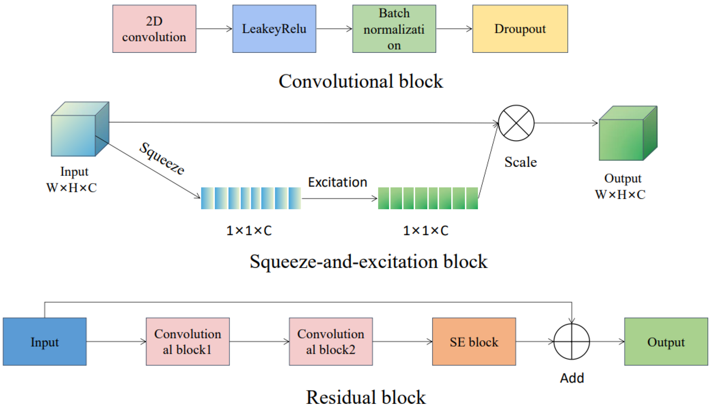
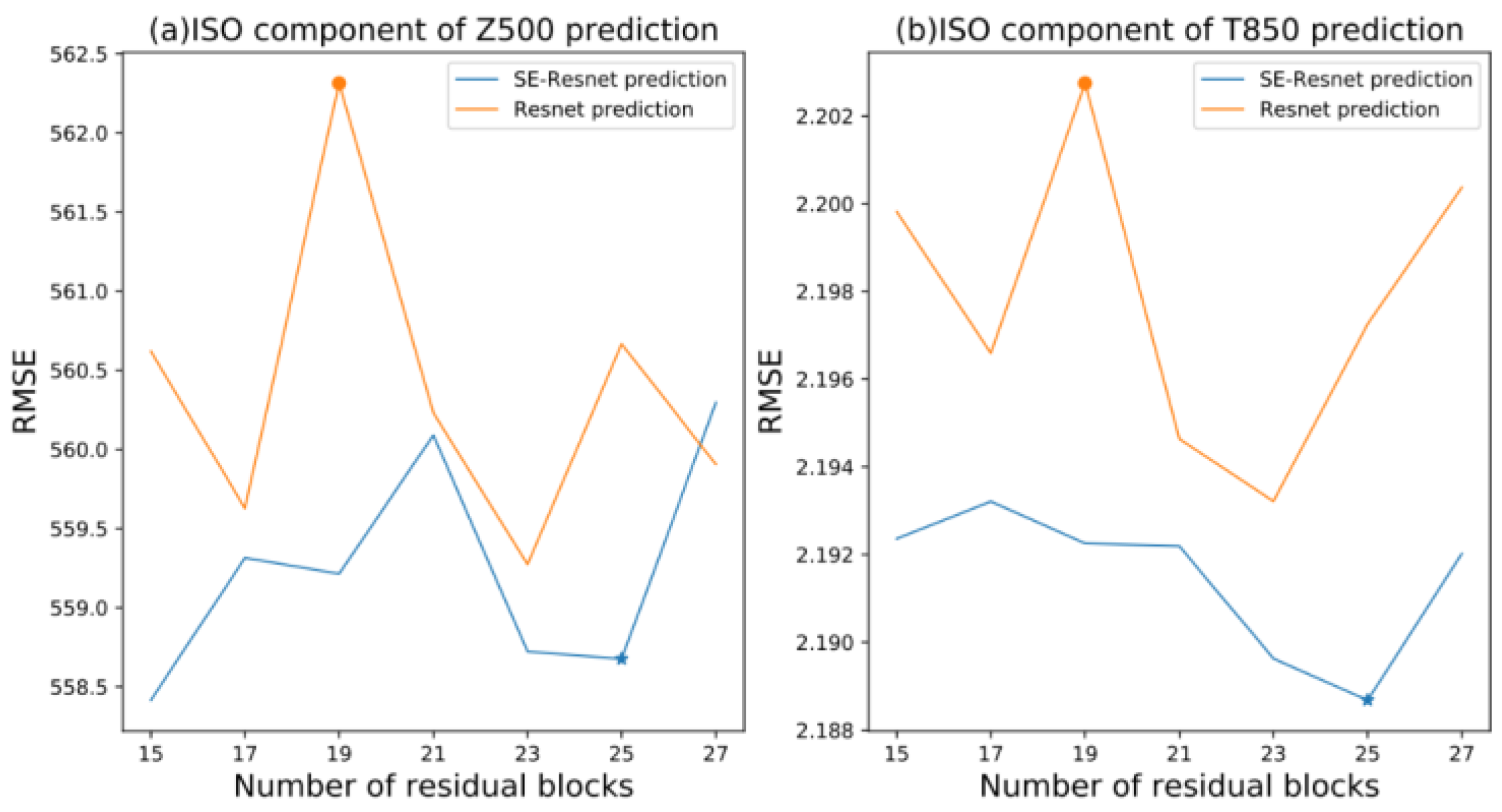
2.2.2. Forecast Model

The original ResNet [37] contains 34 convolution layers and ends with a global average pooling layer and a 1000-way fully connected layer with softmax. There are also shortcuts inserted between the convolution layers, which can be directly used when the input and output are of the same dimensions. The ResNet model used in the study of Rasp and Thuerey (2021b) is further developed based on He’s model [38], and the forecast model used in this paper is developed based on Rasp’s model and is further improved according to the prediction objectives. The specific model structure is shown in Figure 1. The ResNet model in Rasp and Thuerey (2021b) contains 19 residual blocks, which consists of two convolution blocks. The convolution block is defined as a 2D convolution layer, an activation function layer, a batch normalization layer and a dropout layer. All convolutions are padded periodically in the longitudinal direction but with zero in the latitudinal direction.

The SE-ResNet model for this study is a further improvement based on the model above. Both models have a similar structure and use the same convolution block, but in the residual block of the SE-ResNet model, a squeeze-and-excitation block is added, which works as a self-attention mechanism. When there are multiple elements put into the model, the squeeze-and-excitation block can choose the importance of each channel through the squeeze and excitation operations, and the weight coefficient is put on each channel with the scale operation to complete the recalibration of the importance of the original channel [34]. The residual block obtains the final output by adding the output of the squeeze-and-excitation block and the input of the residual block.

In addition, we compared the performance of direct forecast and continuous forecast on the ISO component and found that the results are comparable. Particularly, the average area-weighted root mean squared error (RMSE, as documented in Formula (1) in Section 2.2.3) for 10–30 days of the direct model is 552.48 m² s⁻² (2.17 K), and the average RMSE for 10–30 days of the continuous model is 558.68 m² s⁻² (2.19 K). Therefore, to learn the underlying physical processes, the method of continuous forecast is applied in this paper. We determined the number of residual blocks of the SE-ResNet model as 25 through experiments (Figure 2), where the average RMSE for 10–30 days of the predicted results of Z500 and T850 is the lowest. The other parameters in training the SE-ResNet model are set as follows. The initial learning rate is set to 0.5 × 10⁻⁴, which will be reduced by a factor of 5 once the validation loss does not decrease for 2 epochs. Each residual block contains two convolution blocks with 128 channels. The convolution kernel size is 3. Weight decay is 0.01 used for all layers. The activation function is LeakyReLU. Dropout is set to 0.3.

We also use different test sets to verify the structural differences between the SE-ResNet and ResNet models (

Table 1. Comparison of the average RMSE for 10–30 days of Z500 and T850 achieved with the SE-ResNet and ResNet models (SE-ResNet/ResNet) using different test years.

Test Year	Z500 (Units: m2 s−2)	T850 (Units: K)
(2007, 2008)	561.14/565.21	2.19/2.20
(2009, 2010)	567.92/572.66	2.24/2.26
(2011, 2012)	570.70/574.64	2.18/2.20
(2013, 2014)	556.41/560.09	2.20/2.21
(2015, 2016)	567.05/571.18	2.19/2.20
(2017, 2018)	558.68/562.31	2.19/2.20

) for the cross-validation. The results show that the prediction effect of SE-ResNet is stably better than that of ResNet as the test set changed. Particularly, the average gap for Z500 is 4.03 m² s⁻², and the average gap for T850 is 0.01 K. The table shown below not only indicates that the addition of the SE module can improve the ResNet model to a certain extent but also shows that the superiority is steady, as for all the test subsets, SE-ResNet outperforms ResNet.

2.2.3. Forecast Effect Evaluation Methods

To evaluate the forecast results of the model, RMSE is defined as

$$RMSE=\frac{1}{N_{forecasts}}\sum _i^{N_{forecasts}}\sqrt{N_{lat}{N}_{lon}\sum _j^{N_{lat}}\sum _k^{N_{lon}}L\left(j\right){\left(f_{i,j,k}-t_{i,j,k}\right)}^2}$$

(1)

where f is the prediction result of the model, and t is the filtered ERA5 data of the corresponding time. The RMSE score is a positive value with no upper limit. The smaller the RMSE value is, the better the prediction result of the model is. The anomaly correlation coefficient (ACC) is defined as

$$ACC=\frac{{\sum }_{i,j,k}L\left(j\right){f^{\prime }}_{i,j,k}{t^{\prime }}_{i,j,k}}{\sqrt{{\sum }_{i,j,k}L\left(j\right){f^{\prime 2}}_{i,j,k}{\sum }_{i,j,k}L\left(j\right){t^{\prime 2}}_{i,j,k}}}$$

(2)

where the symbol ′ represents the difference to the climatology. L(j) is the weight factor when latitude is j (unit; °), and L(j) is defined as

$$L\left(j\right)=\frac{\cos \left(lat\left(j\right)\right)}{\frac{1}{N_{lat}}{\sum }_j^{N_{lat}}\cos \left(lat\left(j\right)\right)}$$

(3)

ACC can represent the spatial similarity between two fields. The ACC value should range from −100 to 100 (unit; %). The closer the value of ACC is to 100, the more similar the two fields are.

3. Model Forecast Results

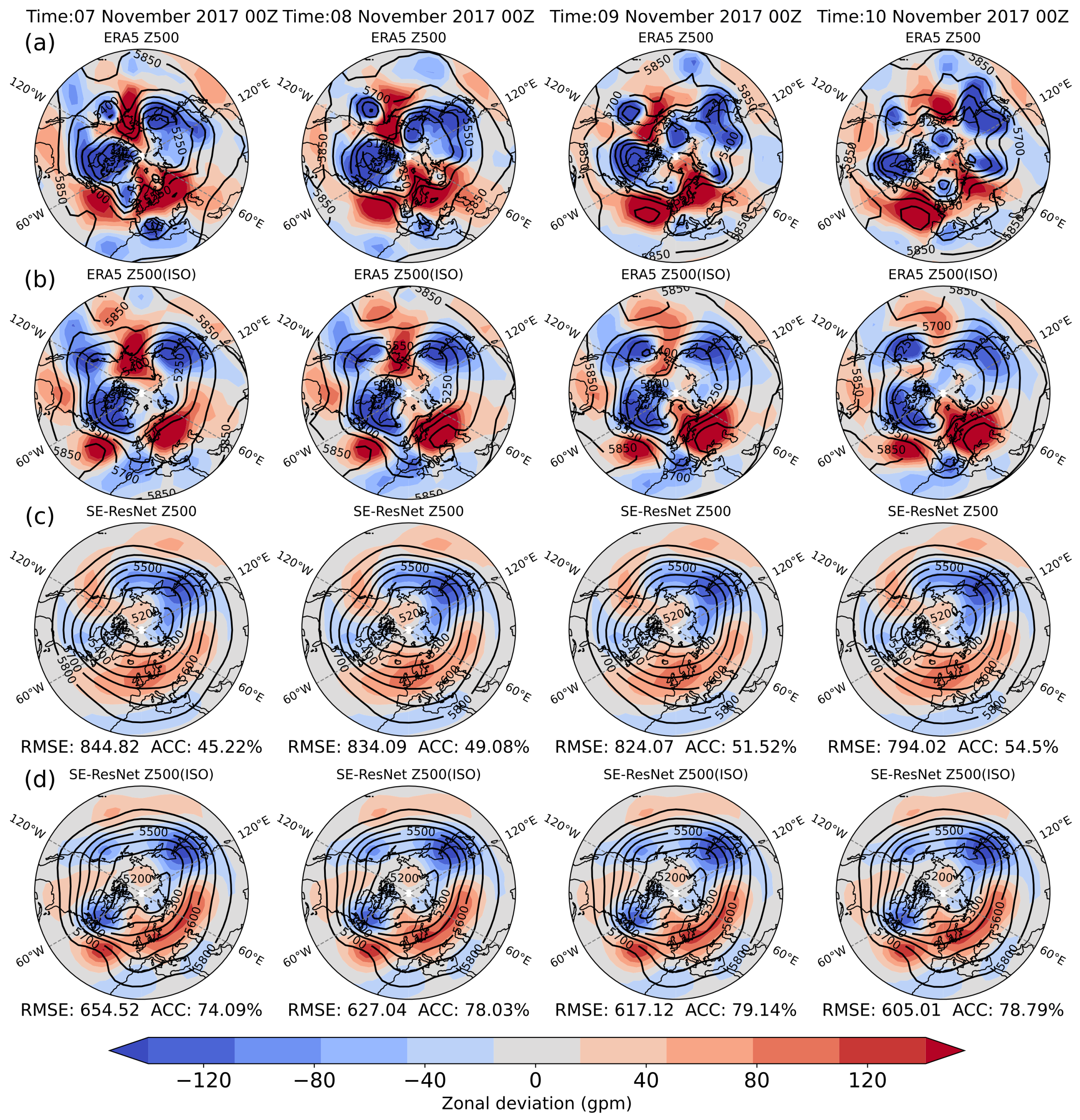
3.1. Prediction Case Analysis: Original Data vs. ISO Component

This paper mainly focuses on the 10–30 day forecast ability of ISO components. To show the importance of ISO components in actual atmospheric changes and the forecast ability of ISO components, Figure 3 compares the zonal deviation of ERA5 and predicted Z500 and its ISO components during 7–19 November 2017. According to the variations in the ERA5 original field (non-ISO) and ERA5 ISO component field over time (Figure 3a,b), the ERA5 ISO components reasonably reflect the main trough–ridge system (Rossby wave) and its characteristics of amplitude and movement of the original Z500 (non-ISO) over time, especially in the middle and high latitudes of the Northern Hemisphere. The systems, including troughs along the western coast of Europe, East Asia, the Gulf of Alaska and northeastern Canada as well as ridges in the midlatitude North Atlantic, Urals and south of the Aleutian Islands, are all well shown in the figure. However, the amplitudes of the ISO components are slightly smaller than the weather fluctuations with a mean variance contribution of 26.67%, indicating that the ISO components are of paramount importance to actual atmospheric variation. In fact, the ISO components are good indicators of large-scale persistent circulation systems and the associated extreme weather and climate events [39].

Two prediction processes of the models are compared in Figure 3c,d. The former uses the original data (non-ISO data) to train the model and filters the model output to obtain the prediction result, while the latter uses the ISO data to train the model and takes the model output as the prediction result. Predictions at forecast lead times of 10–22 days based on the original data (non-ISO) and ISO components can both well reflect the variation characteristic of the deep troughs in the East Asian region and northeast Canada. The variation characteristics of the shallow trough in the Gulf of Alaska and the ridges on the west coast of North America and northwest Eurasia can also be reasonably reflected, but the prediction results are weaker in oscillation variation and smoother in streamlines than the midlatitude atmospheric fluctuations described by the ERA5 ISO components (Figure 3c,d). The global mean RMSE of the prediction driven by ISO components for 10–22 days is 549.27 m² s⁻² (not shown), which is notably better than the CFSv2 prediction in the same period (RMSE: 563.32 m² s⁻²). Interestingly, the model prediction results of Z500 driven by the original data (unfiltered non-ISO data) have a similar spatial form to the results predicted using ISO components, showing a distinct “low-frequency” (smoothened) feature. Furthermore, in this case, the Z500 ISO values predicted by the ISO components are closer to the ERA5 ISO components with a mean RMSE of 577.94 m² s⁻². (We only show analysis for 4 days here due to limited space. For the rest of the days, please refer to Figure A2, Figure A3, Figure A4, Figure A5 and Figure A6 in the Appendix part). Similarly, the T850 ISO values predicted by the ISO components are in better agreement with the ERA5 ISO components (Figure A2). The global mean RMSE for the ISO components at 10–22 days is 2.16 K, which is significantly lower than the prediction driven by the original data (non-ISO) (2.30 K). This may be because the degrees of freedom and complexity of the ISO components are lower than those of the original variables (non-ISO), which could lead to the learning ability of the model based on ISO components being better than the model driven by the original data (non-ISO).

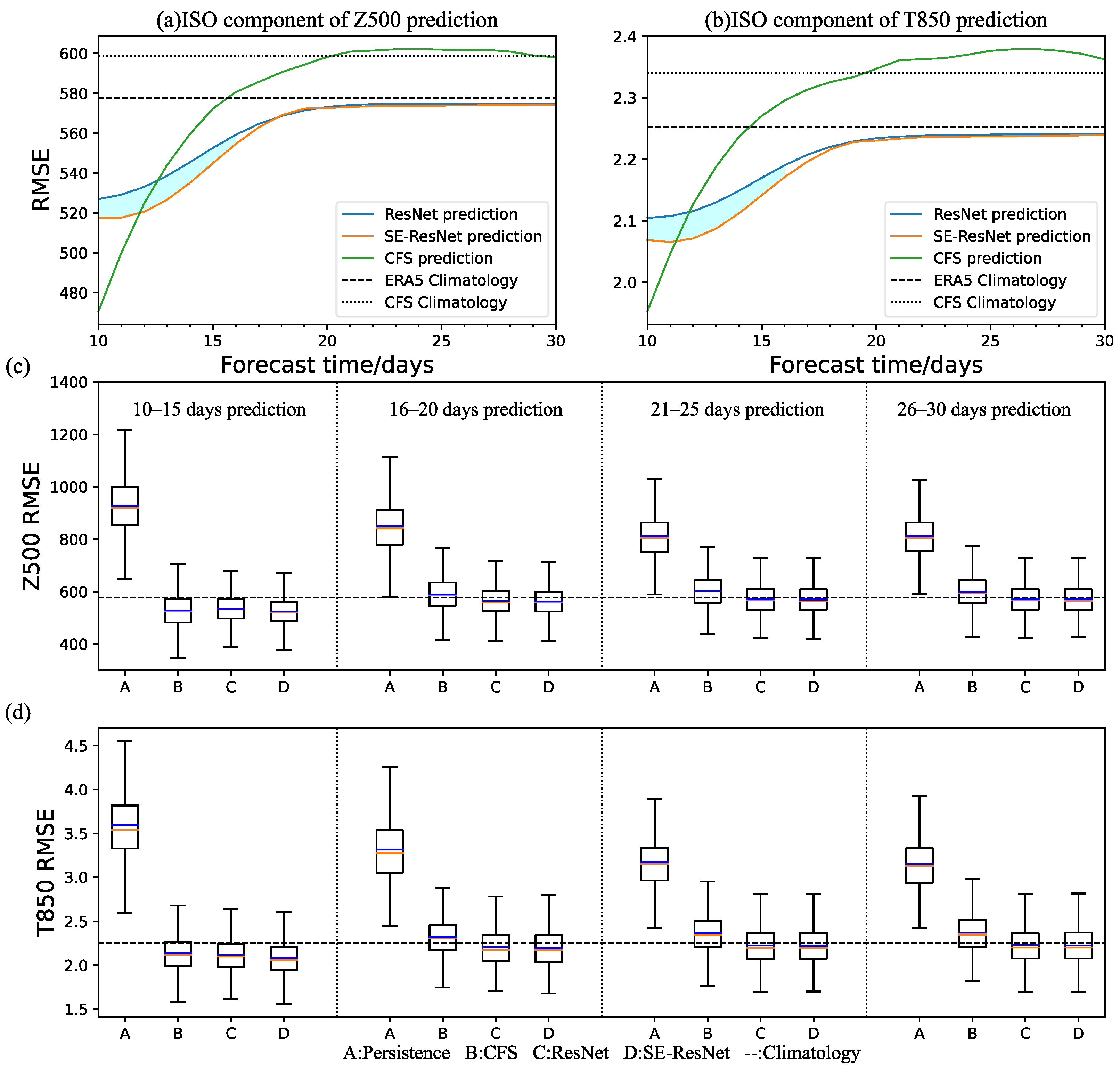
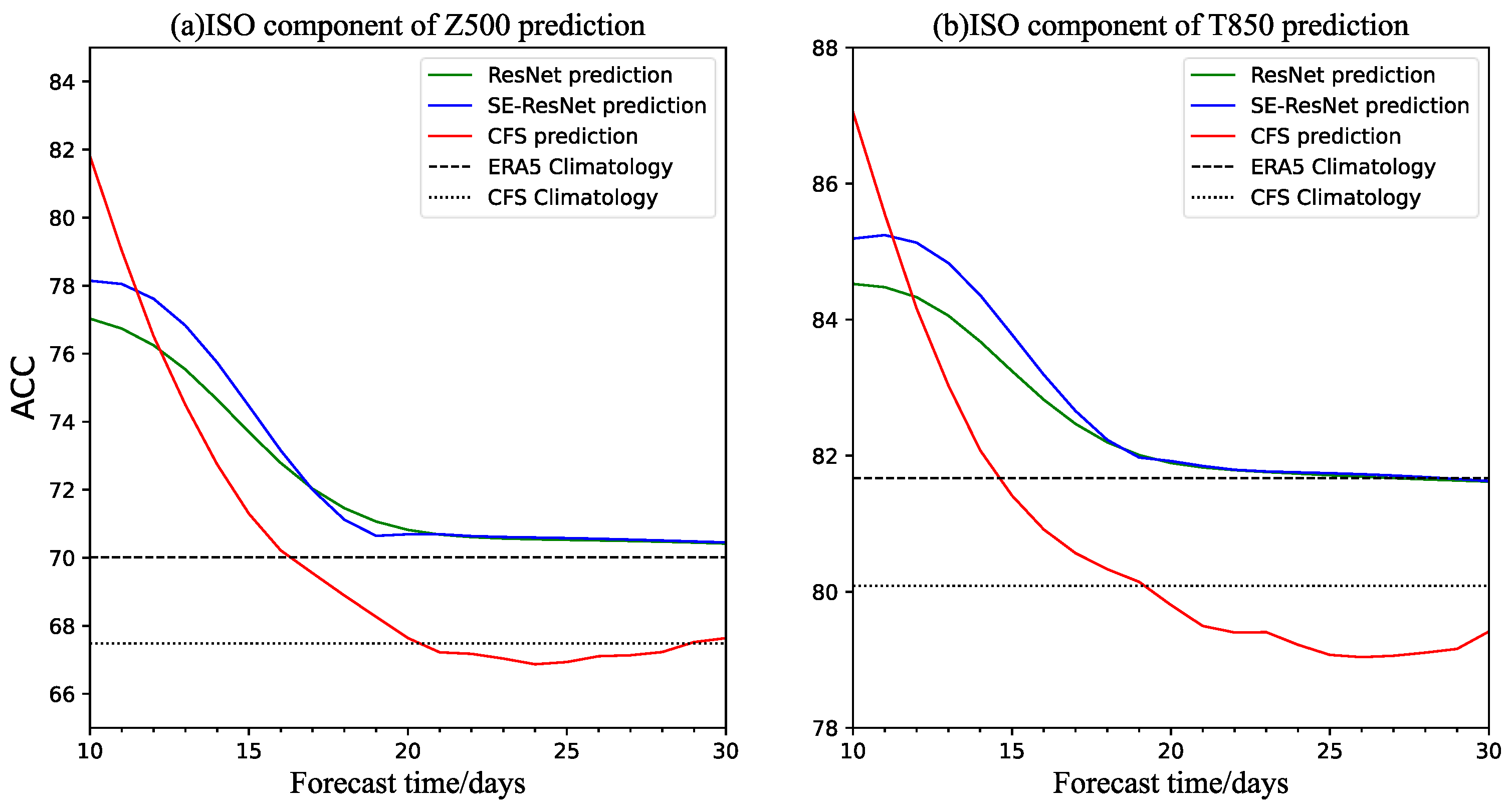
3.2. Overall Evaluation of the Model

To reflect the long-term overall prediction result of the model, Figure 4 presents the RMSE of the model’s prediction results for the global average Z500 and T850 ISO components at forecast lead times of 10–30 days in 2017–2018 (a total of 2920 samples). For the ISO component forecast, the RMSE values of the CFSv2, ResNet and SE-ResNet results of global Z500 all increase with the forecast lead times. The increase rate is larger in the lead time range of 10–20 days and flattens after that with a smaller decrease rate. ResNet and SE-ResNet perform better than the ERA5 climatological forecast (mean RMSE: 577.62 m² s⁻²), persistence forecast (calculated from filtered ERA5 data, the worst prediction, mean RMSE: 859.35 m² s⁻²) and CFSv2 climatological forecast (mean RMSE: 598.88 m² s⁻²) over the 10–30 day forecast lead times. It is noteworthy that the average RMSE of the CFSv2 model is larger than that of the ResNet model and the SE-ResNet model when the forecast lead times are more than 13 days, indicating that, although the prediction of global atmospheric circulation and its ISO components based on the dynamic seasonal climate prediction system still has a great advantage in the lead time range of 10–13 days, its prediction ability beyond 13 days is weaker than the data-driven ResNet model and the SE-ResNet model. Compared with the ERA5 climatological forecast, the CFSv2 model has lower prediction skills beyond 16 days. Moreover, the average RMSE of the SE-ResNet model is 0.65% lower than that of the ResNet model through lead times of 10–30 days. This is an improvement upon the ResNet model because of the squeeze-and-excitation block, which optimizes the output based on the importance and weight of each factor when using multiple inputs.

As observed from the RMSE boxplot of the ISO components of Z500 every 5 days (Figure 4c), the RMSE of 75% of the samples predicted by the deep-learning model is below the ERA5 climatological forecast in 10–15 days, and the RMSE of more than 50% of the samples predicted remains below the ERA5 climatological forecast after that. The CFSv2 model predictions have more than 50% of the samples with a higher RMSE than the ERA5 climatological forecast in forecast lead times of 16–20 days and beyond. The persistence forecast is the worst with the RMSE of all the predicted samples being higher than the ERA5 climatological forecast, and the RMSE of more than 75% of the samples is above 1000 m² s⁻². Not surprisingly, the SE-ResNet model has the “best” inaccurate forecast case (RMSE: 672.01 m² s⁻²), followed by the ResNet model, CFSv2 model and persistence forecast. For the “best” accurate forecast case, SE-ResNet and ResNet are close, outperforming the CFSv2 model and persistence forecast beyond 16 days. On the other hand, the “best” accurate forecast case of each model is obtained from the lead time range of 10–15 days, where the CFSv2 model has a best case with an RMSE of 346.38 m² s⁻².

For the global average ISO components of T850, the prediction result of each model is similar to the prediction results of Z500. As shown in Figure 4b, the SE-ResNet model is still the model with the highest forecasting skills with an average RMSE 0.45% lower than the ResNet model through forecast lead times of 10–30 days. Both the SE-ResNet model and ResNet model are superior to ERA5 climatological forecasts, and their RMSE beyond 12 days is significantly lower than that of the CFSv2 model, which is inferior to ERA5 climatological forecasts beyond 14 days. In the RMSE boxplot of the ISO components of T850 every 5 days (Figure 4d), the overall prediction performance of SE-ResNet and ResNet outperform the CFSv2 model and persistence forecast. The SE-ResNet model has the “best” inaccurate prediction case (RMSE: 2.60 K), followed by the ResNet model, CFSv2 model and persistence forecast. For the “best” accurate prediction case, the SE-ResNet, ResNet and CFSv2 models are close, but the RMSE value of the CFSv2 model increases slightly beyond 21 days.

To verify the composite difference between the three models, we conducted the student’s t-test on the prediction effects between the SE-ResNet model and the other two models. The results showed that the SE-ResNet model and ResNet model passed the significance test (α = 0.05) within 10–16 days. Moreover, the SE-ResNet model and CFSv2 model passed the significance test within 10–30 days.

Table 2. Comparison of the average RMSE (10–20/21–30/10–30 days) of Z500 and T850 achieved with the different models.

Model	Z500 (Units: m2 s−2)			T850 (Units: K)
	10–20	21–30	10–30	10–20	21–30	10–30
CFSv2	556.44 *	600.98 *	577.65 *	2.22 *	2.37 *	2.29 *
ResNet	551.15 *	574.59	562.31 *	2.17 *	2.24	2.20 *
SE-ResNet	544.89	573.84	558.68	2.14	2.24	2.19

* represents the RMSE of the corresponding model and SE-ResNet model prediction results passing the average test (α = 0.05).

summarizes the average RMSE of Z500 and T850 achieved with the different models to show the average prediction effect of the model over specific lead time periods. It can be found that the SE-ResNet model is superior to the other models in all three lead time periods. The difference between the SE-ResNet and ResNet models is relatively large in 10–20 days and passes the mean test in general. However, with the extension of the forecast time, the prediction effects of the two models are close to the ERA5 climatology prediction, and the difference gradually reduces, which leads to a smaller average increase in the SE-ResNet model within 10–30 days. The CFSv2 model performs the worst, passing the significance test for all three time periods, which indicates a significant improvement in the predictive performance of the SE-ResNet model over the CFSv2 model.

To quantitatively show the spatial similarity between the ISO components predicted by the different models and the ERA5 ISO components, the sequence of the global average ACC of the predicted ISO components for Z500 and T850 with different forecast lead times is given in Figure 5. The results are similar to the RMSE results analysis, and the ACC scores of the deep-learning models are significantly superior to the other models beyond 13 days. Among them, the spatial similarity between the predicted ISO components of the SE-ResNet model and the ERA5 ISO components is the highest, and the ACC of Z500 and T850 for 10–30 days is 72.58% and 82.75%, respectively. Unsurprisingly, its prediction result for 10–30 days is higher than that of the ERA5 climatological forecast. The ResNet model has the second highest ACC skills with an average ACC of 72.25% for Z500 and 82.51% for T850 over 10–30 days. The ACC scores for the Z500 and T850 ISO components predicted by CFSv2 are lower than the ACC score of the ERA5 climatological forecast in approximately 17 and 15 days, respectively, and lower than the ACC scores of the two deep-learning models beyond forecast lead times of 13 days. The CFSv2 ACC score of Z500 and T850 in 10–30 days is 70.11% and 80.8%, respectively. The ACC scores of the persistence forecast are the worst with an average ACC of 47.48% and 65.28% for Z500 and T850 during 10–30 days, respectively.

From the perspective of the global average, the above section shows that the prediction performance of the SE-ResNet model is better than that of CFSv2 for the Z500 and T850 ISO components during 14–30 days. To further show the difference in the prediction effects between the CFSv2 forecast and SE-ResNet forecast at different latitudes, Figure 6 demonstrates the difference between the zonal average RMSE of the prediction results of the two models under different forecast lead times. The large RMSE difference between the two models mainly occurs in the extratropical region of the two hemispheres, while the difference is relatively small in the tropical region. In general, CFSv2 has a large advantage in the prediction of the Z500 and T850 ISO components when the forecast lead time is less than 10 days. However, when the forecast lead time is beyond 10 days, the prediction results of the SE-ResNet model are stably better than those of CFSv2, which is consistent with the analysis results of the global average (Figure 4). Specifically, the RMSE predicted by the SE-ResNet model for Z500 (T850) is, on average, 26.18 m² s⁻² (0.14 K) lower than that of CFSv2 in the 20–80° region when the forecast lead time is beyond 10 days.

Since planetary waves are the main drivers of atmospheric circulation at middle and high latitudes and regional weather/climate anomalies, the enhancement of planetary wave activity is closely related to long-term extreme climate events [39,40]; therefore, the difference between CFSv2 and SE-ResNet in the extratropical region may be due to the difference in the prediction skills of planetary waves. Figure 7a,b further show the RMSE and ACC of the CFSv2 and SE-ResNet models for planetary waves with wavenumbers of 3–8 at 30–70° N in the Northern Hemisphere compared with filtered ERA5 data. It can be clearly observed that the SE-ResNet model has a good skill in the prediction of planetary waves with wavenumbers of 3–8 beyond 12 days. The average RMSE of the SE-ResNet model is 529.05 m² s⁻² during the forecast lead times of 12–25 days, which is significantly lower than that of the ERA5 climatology (551.39 m² s⁻²) and CFSv2 model (559.95 m² s⁻²). Compared with the CFSv2 model, the SE-ResNet model is 30.90 m² s⁻² lower on average at 12–25 days, which is equivalent to the average zonal deviation of the two models shown in Figure 6a, indicating that the difference in the prediction effect for extratropical Z500 is mainly due to the difference in prediction performance for planetary waves. At the same time, the ACC results also show that the performance of the SE-ResNet model is better than that of the ERA5 climatology (82.29%) during 12–25 days, while the CFSv2 model has low prediction skills beyond 16 days.

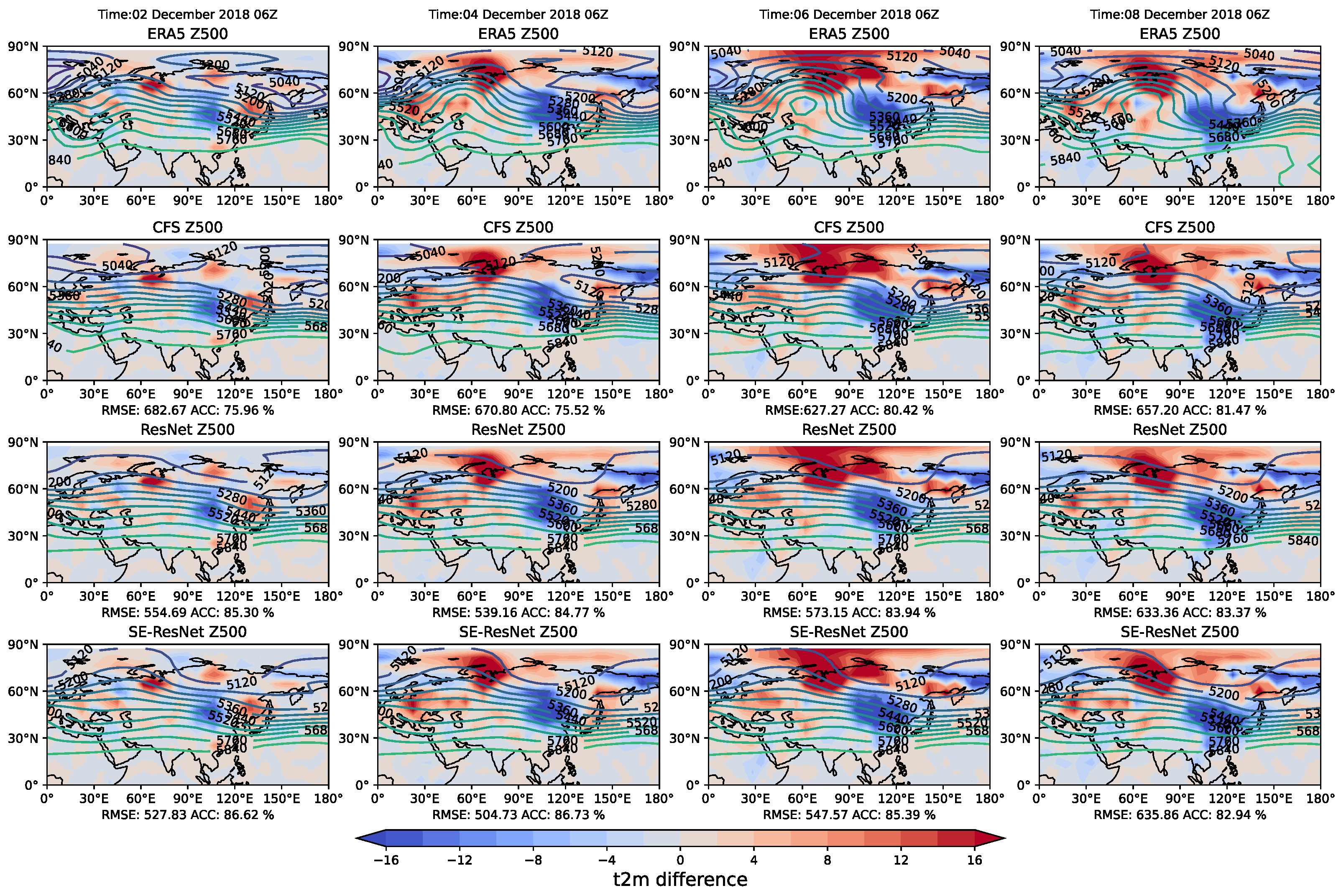
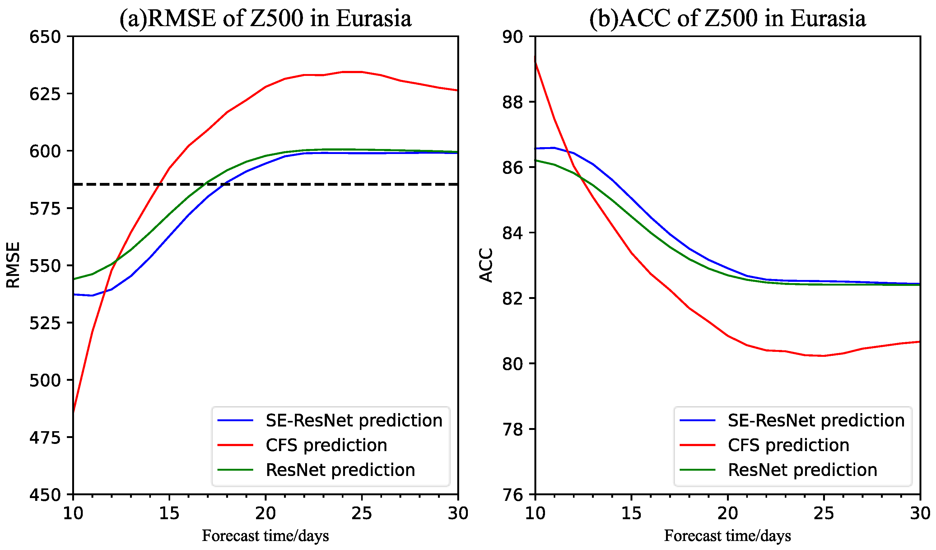
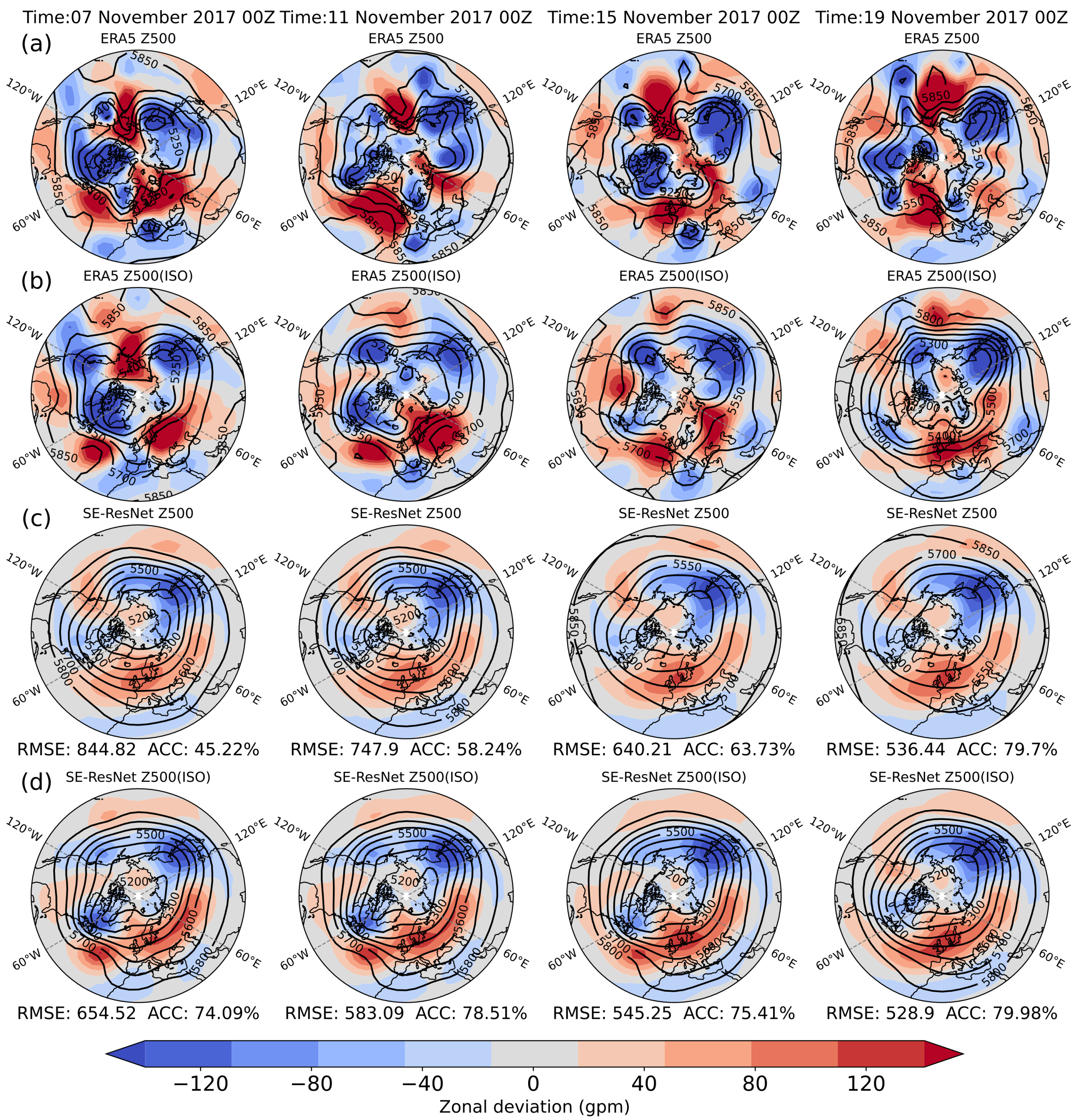
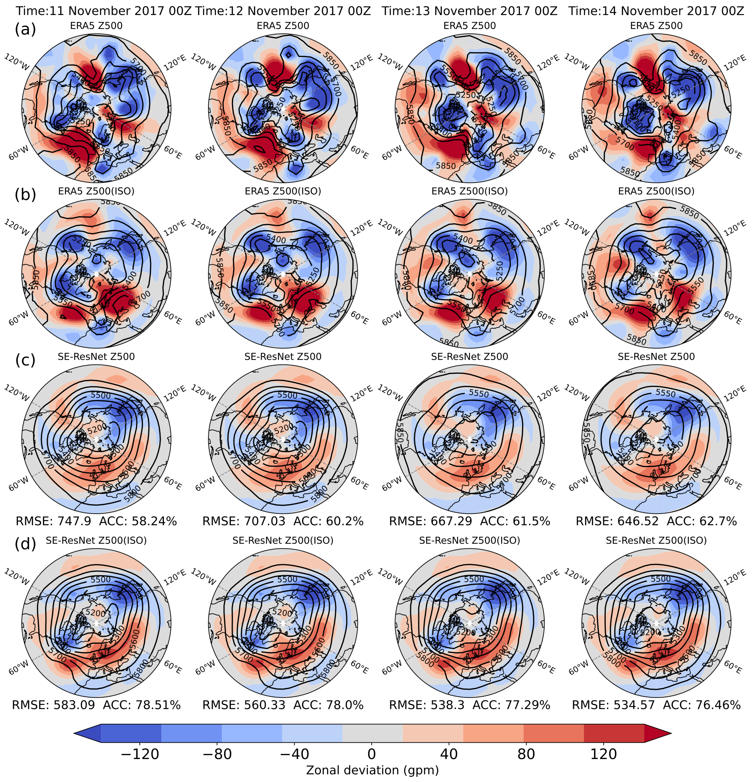
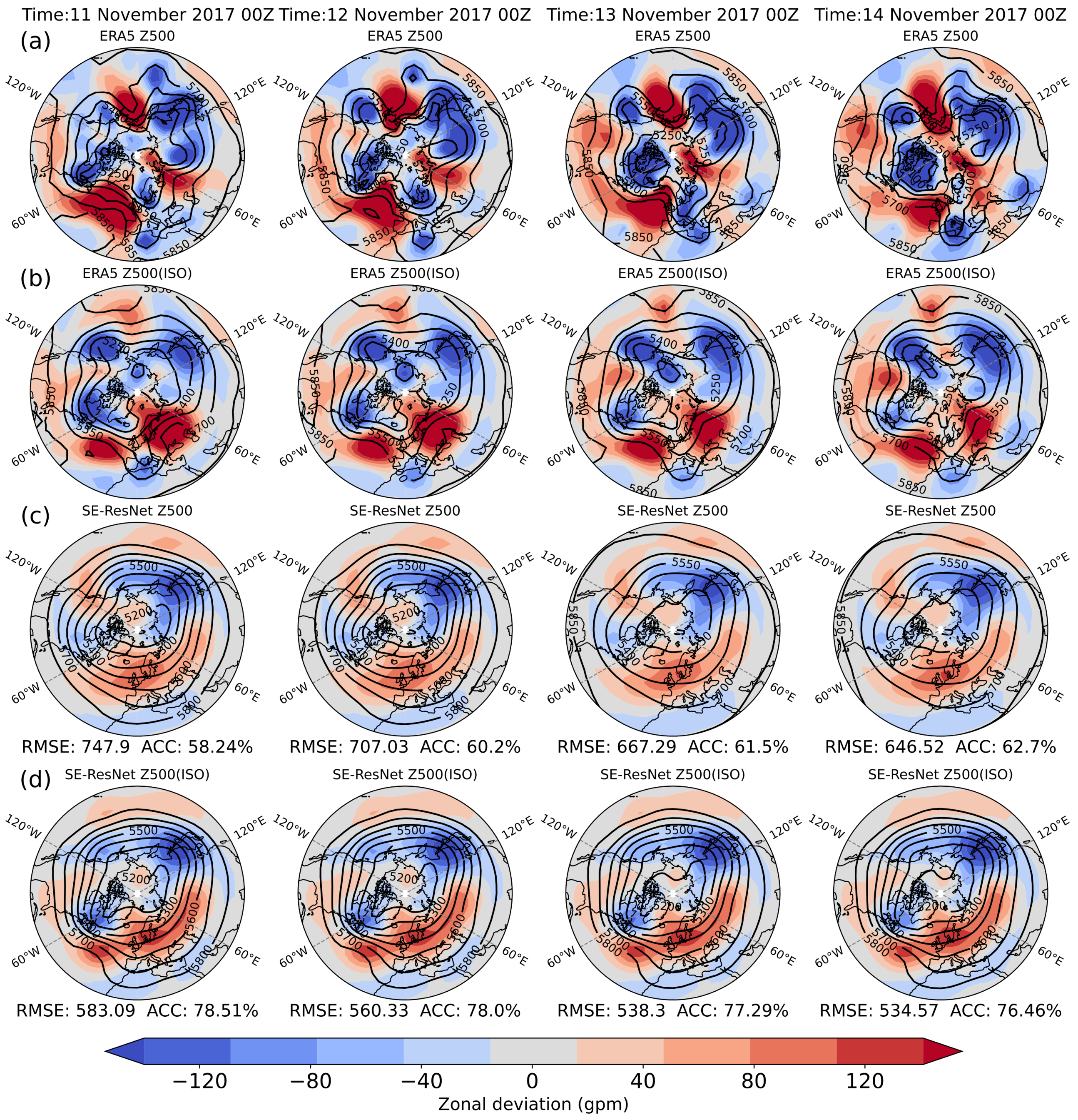
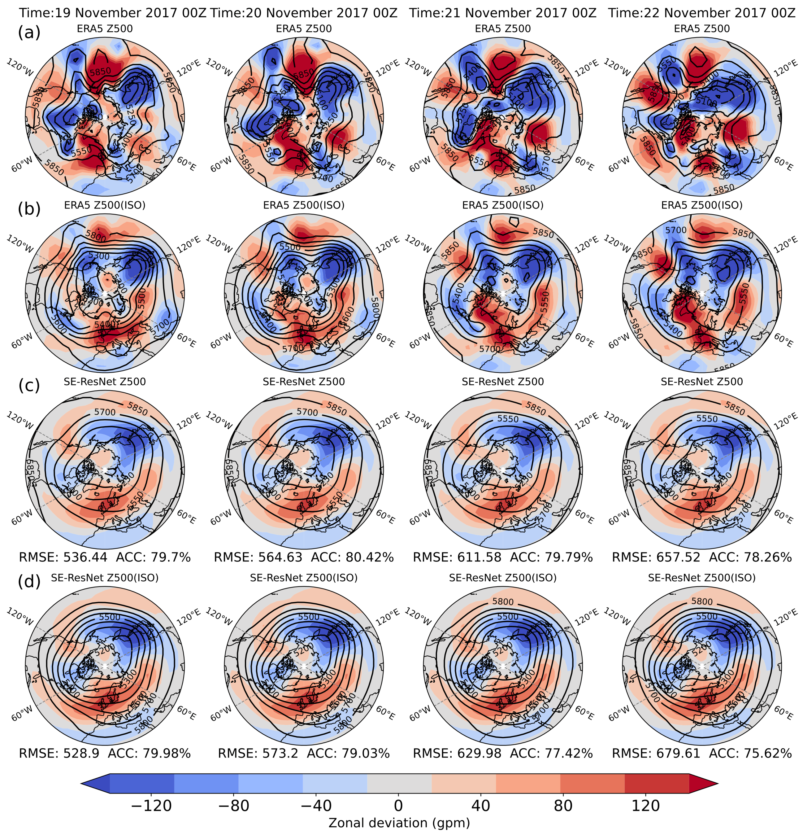
3.3. Prediction and Evaluation of the 500 hPa Circulation Situation in the Eurasian Region

Focusing on the reliability of the 10–30 day forecast of regional upper-level circulation with the different methods, the following section uses the Eurasian region as an example to give an individual case and their overall prediction performance. Figure 8 first shows the Z500 ISO components of a cold wave weather process in Eurasia from 2 to 8 December 2018 and the difference in the ERA5 ground 2 m temperature between the schematic time and 06 UTC on 1 December 2018. This event was a continuous large-scale cold wave affecting East Asia with the cooling area mainly concentrated in eastern China, the Korean Peninsula and Japan, and the local temperature dropped up to 10.12 K (23.60 K) within 24 (72) hours. During this process, the characteristics of planetary wave activity are obvious and are mainly caused by the continuous maintenance and strengthening of the blocking high near the Ural Mountains, leading to the deepening and development of the downstream East Asian trough. Meanwhile, along with the continuous eastward movement of the low trough in Central and Western Europe, a large amount of cold air from the northwest entered East Asia, resulting in widespread and persistent cooling. According to the prediction results, the three models reflect the phase and propagation characteristics of the planetary wave well and clearly represent the maintenance and development of the blocking high near the Ural Mountains and the deepening of the East Asian trough. However, because the model only focuses on the ISO components, the amplitude of the wave oscillation is relatively smaller than that of the ERA5 ground truth. From the perspective of RMSE and ACC scores, the prediction results of the SE-ResNet model over 10 days are superior to those of the CFSv2 model. In particular, after 6 December, the contour lines of the CFSv2 model’s prediction results near the Ural Mountains gradually become flat, and the position of the high-pressure ridge appears at approximately 90° E, which is to the east of the real position. Compared with the ResNet model, the SE-ResNet model is only slightly worse at 06 UTC on 8 December and is better than the ResNet model at other times with lower RMSE and larger ACC values.

To evaluate the overall prediction effect of the different models in the Eurasian region, the average RMSE and ACC of the Z500 ISO components with the forecast lead times are shown in Figure 9. It can be inferred that the SE-ResNet model performs best in the overall prediction of upper-level circulation over the Eurasian region. The average RMSE and ACC of 10–30 days are 580.34 m² s⁻² and 83.78%, respectively. The ResNet model is slightly worse than the SE-ResNet model with a mean RMSE and ACC of 585.03 m² s⁻² and 83.51% for 10–30 days, respectively. The forecast skill of the CFSv2 model is worse than that of the deep-learning model beyond 13 days, and the average RMSE and ACC at 10–30 days are 603.85 m² s⁻² and 82.31%, respectively. Similar to the global prediction results, the RMSE and ACC predicted by CFSv2 show a large variation rate over 20 days, while it tends to be flat beyond that with a smaller decrease rate over time. We also notice that all the predictions over Eurasia are worse than the climatological forecast beyond 20 days. We think that it could be due to the atmospheric instability over the middle and high latitudes, as the Eurasia continent is a large piece of land with inconsistency in the characteristics of the underlying surface and atmospheric fluctuation is frequent over this region. Compared to the global prediction, where vast sea surface covers more than 70% of the underlying surface, having a relatively consistent characteristic, there will be more significant atmospheric variations over Eurasia.

4. Discussion and Conclusions

In this paper, we use ISO components of atmospheric signals to train the SE-ResNet machine-learning model to forecast the global Z500 and T850 situation in the next 1–30 days and compare the prediction results with the ResNet and CFSv2 models. In this study, we choose RMSE and ACC as our evaluation metrics, and our model shows superiority compared to the other models, including CFSv2 and the original ResNet model. Compared with the previous deep-learning model, the forecast model used in this study makes the following important improvements. (1) As the prediction object gradually tends to become the low-frequency component with the increase in the forecast time within the subseasonal timescale, the ISO components are directly used to train the forecast model. (2) Adding a self-attention mechanism optimizes the importance of different factor channels in the model. We also noticed that recent AI weather forecast models, like Pangu [21] and Fengwu [22], mainly focus on the weather forecast with lead times of 1–7 days; therefore, we hope our technique of self-attention and ISO extraction may provide inspiration for them to tackle forecasts with longer lead times.

We studied two indicators, RMSE and ACC, to evaluate the predictive performance of the model, and the results show that the SE-ResNet model is significantly better than the CFSv2 model in forecast lead times of 10–30 days. It is worth noting that the deep-learning model is not endowed with meteorological constraints internally, but we still try to analyze the interpretability of its prediction results. The difference between the CFSv2 model and SE-ResNet model mainly occurs in the extratropical region and is small in the tropical region. Moreover, the SE-ResNet model has good performance in the prediction of planetary waves with wavenumbers of 3–8 beyond 12 days, which also leads to the difference in the prediction performance of the models in the extratropical regions. As an issue to focus on, the variation characteristics of planetary waves are closely related to the occurrence and development process of weather. Not surprisingly, the data-driven model we developed in this study has a reliable reflection on the phase and propagation characteristics of planetary waves at forecast lead times of 11–30 day.

It should be noted that when latitude-weighted RMSE is used as the loss function training model in this paper, the predicted circulation oscillation features tend to become smooth over the forecast duration. As an optimization of the model loss function, for example, the weight of the loss function can be set to increase with the forecast time or use a multi-time step-loss function [41] to help improve the stability and accuracy of long-term prediction. On the other hand, meteorological elements are closely correlated with each other. Although deep learning provides a new method for the prediction of weather and climate evolution, the prediction objects in this study are limited to Z500 and T850 and are not necessarily constrained by the physical relationship between multiple elements [31]; therefore, using a machine-learning framework based on physical models [42,43] or combining dynamic models with deep-learning models [44] may help improve the reliability and authenticity of subseasonal forecast models. Furthermore, recent studies have shown that probabilistic weather prediction makes it possible to calculate the uncertainty and skill index of neural network prediction [45], which also provides a reference basis for probabilistic prediction within the subseasonal timescale.

References

1. Jin, R.; Ma, J.; Ren, H.; Yin, S.; Cai, X.; Huang, W. Advances and development countermeasures of 10~30 days extended-range forecasting technology in China. Adv. Earth Sci. 2019, 34, 814–825. (In Chinese) [Google Scholar] [CrossRef]
2. Hoskins, B.J. The potential for skill across the range of the seamless weather-climate prediction problem: A stimulus for our science. Q. J. R. Meteorol. Soc. 2013, 139, 573–584. [Google Scholar] [CrossRef]
3. Lorenz, E.N. Deterministic nonperiodic flow. J. Atmos. Sci. 1963, 20, 130–141. [Google Scholar] [CrossRef]
4. Mayer, K.J.; Barnes, E.A. Subseasonal Forecasts of Opportunity Identified by an Explainable Neural Network. Geophys. Res. Lett. 2021, 48, e2020GL092092. [Google Scholar] [CrossRef]
5. Srinivasan, V.; Khim, J.; Banerjee, A.; Ravikumar, P. Subseasonal climate prediction in the western US using Bayesian spatial models. In Proceedings of the 37th Conference on Uncertainty in Artificial Intelligence, Virtual, Online, 27–30 July 2021; Available online: https://auai.org/uai2021/pdf/uai2021.361.pdf (accessed on 12 December 2021).
6. Vitart, F.; Ardilouze, C.; Bonet, A.; Brookshaw, A.; Chen, M.; Codorean, C.; Déqué, M.; Ferranti, L.; Fucile, E.; Fuentes, M.; et al. The Subseasonal to Seasonal (S2S) Prediction Project Database. Bull. Amer. Meteor. Soc. 2017, 98, 163–173. [Google Scholar] [CrossRef]
7. Mariotti, A.; Ruti, P.M.; Rixen, M. Progress in subseasonal to seasonal prediction through a joint weather and climate community effort. NPJ Clim. Atmos. Sci. 2018, 1, 4. [Google Scholar] [CrossRef]
8. Robertson, A.W.; Kumar, A.; Peña, M.; Vitart, F. Improving and Promoting Subseasonal to Seasonal Prediction. Bull. Amer. Meteor. Soc. 2015, 96, ES49–ES53. [Google Scholar] [CrossRef]
9. Li, W.; Hsu, P.C.; He, J.; Zhu, Z.; Zhang, W. Extended-range forecast of spring rainfall in southern china based on the madden–julian oscillation. Meteor. Atmos. Phys. 2016, 128, 331–345. [Google Scholar] [CrossRef]
10. Zhu, Z.; Li, T.; Bai, L.; Gao, J. Extended-range forecast for the temporal distribution of clustering tropical cyclogenesis over the western north pacific. Theor. Appl. Climatol. 2017, 130, 865–877. [Google Scholar] [CrossRef]
11. Mouatadid, S.; Orenstein, P.; Flaspohler, G.; Cohen, J.; Oprescu, M.; Fraenkel, E.; Mackey, L. Adaptive bias correction for improved subseasonal forecasting. Nat. Commun. 2023, 14, 3482. [Google Scholar] [CrossRef]
12. van Straaten, C.; Whan, K.; Coumou, D.; van den Hurk, B.; Schmeits, M. Using Explainable Machine Learning Forecasts to Discover Subseasonal Drivers of High Summer Temperatures in Western and Central Europe. Mon. Weather Rev. 2022, 150, 1115–1134. [Google Scholar] [CrossRef]
13. Zhu, H.; Wheeler, M.C.; Sobel, A.H.; Hudson, D. Seamless precipitation prediction skill in the tropics and extratropics from a global model. Mon. Weather Rev. 2014, 142, 1556–1569. [Google Scholar] [CrossRef]
14. Zhang, D.; Zheng, Z.; Chen, L.; Zhang, P. Advances on the Predictability and Prediction Methods of 10-30 d Extended Range Forecast. J. Appl. Meteor. Sci. 2019, 30, 416–430. (In Chinese) [Google Scholar] [CrossRef]
15. Hsu, P.C.; Li, T.; You, L.; Gao, J.; Ren, H.L. A spatial–temporal projection model for 10–30 day rainfall forecast in south China. Clim. Dyn. 2015, 44, 1227–1244. [Google Scholar] [CrossRef]
16. Wang, Q.; Chou, J.; Feng, G. Extracting predictable components and forecasting techniques in extended-range numerical weather prediction. Sci. China Earth Sci. 2014, 57, 1525–1537. [Google Scholar] [CrossRef]
17. Lu, C.; Kong, Y.; Guan, Z. A mask R-CNN model for reidentifying extratropical cyclones based on quasi-supervised thought. Sci. Rep. 2020, 10, 15011. [Google Scholar] [CrossRef] [PubMed]
18. Lagerquist, R.; Mcgovern, A.; Gagne, D.J. Deep learning for spatially explicit prediction of synoptic-scale fronts. Wea. Forecast. 2019, 34, 1137–1160. [Google Scholar] [CrossRef]
19. Lagerquist, R.; Allen, J.T.; McGovern, A. Climatology and Variability of Warm and Cold Fronts over North America from 1979 to 2018. J. Clim. 2020, 33, 6531–6554. [Google Scholar] [CrossRef]
20. Ravuri, S.; Lenc, K.; Willson, M.; Kangin, D.; Lam, R.; Mirowski, P.; Fitzsimons, M.; Athanassiadou, M.; Kashem, S.; Madge, S.; et al. Skilful precipitation nowcasting using deep generative models of radar. Nature 2021, 597, 672–677. [Google Scholar] [CrossRef]
21. Bi, K.; Xie, L.; Zhang, H.; Chen, X.; Gu, X.; Tian, Q. Accurate medium-range global weather forecasting with 3D neural networks. Nature 2023, 619, 533–538. [Google Scholar] [CrossRef]
22. Chen, K.; Han, T.; Gong, J.; Bai, L.; Ling, F.; Luo, J.J.; Chen, X.; Ma, L.; Zhang, T.; Su, R.; et al. FengWu: Pushing the Skillful Global Medium-range Weather Forecast beyond 10 Days Lead. arXiv 2023, arXiv:2304.02948. [Google Scholar]
23. Song, K.; Yu, X.; Gu, Z.; Zhang, W.; Yang, G.; Wang, Q.; Xu, C.; Liu, J.; Liu, W.; Shi, C.; et al. Deep Learning Prediction of Incoming Rainfalls: An Operational Service for the City of Beijing China. In Proceedings of the 2019 International Conference on Data Mining Workshops (ICDMW), Beijing, China, 8–11 November 2019. [Google Scholar] [CrossRef]
24. Sønderby, C.K.; Espeholt, L.; Heek, J.; Dehghani, M.; Oliver, A.; Salimans, T.; Agrawal, S.; Hickey, J.; Kalchbrenner, N. MetNet: A Neural Weather Model for Precipitation Forecasting. arXiv 2020, arXiv:2003.12140. [Google Scholar]
25. Weyn, J.A.; Durran, D.R.; Caruana, R.; Cresswell-Clay, N. Sub-seasonal forecasting with a large ensemble of deep-learning weather prediction models. J. Adv. Model. Earth Syst. 2021, 13, e2021MS002502. [Google Scholar] [CrossRef]
26. Rasp, S.; Thuerey, N. Data-driven medium-range weather prediction with a resnet pretrained on climate simulations: A new model for weatherbench. J. Adv. Model. Earth Syst. 2021, 13, e2020MS002405. [Google Scholar] [CrossRef]
27. Jin, W.; Zhang, W.; Hu, J.; Weng, B.; Huang, T.; Chen, J. Using the Residual Network Module to Correct the Sub-Seasonal High Temperature Forecast. Front. Earth Sci. 2021, 9, 760766. [Google Scholar] [CrossRef]
28. Rasp, S.; Dueben, P.D.; Scher, S.; Weyn, J.A.; Thuerey, N. Weatherbench: A benchmark data set for data-driven weather forecasting. J. Adv. Model. Earth Syst. 2020, 12, e2020MS002203. [Google Scholar] [CrossRef]
29. Mathieu, M.; Couprie, C.; LeCun, Y. Deep multi-scale video prediction beyond mean square error. arXiv 2015, arXiv:1511.05440. [Google Scholar]
30. Slingo, J.M.; Bates, K.R.; Nikiforakis, N.; Piggott, M.D.; Roberts, M.J.; Shaffrey, L.C.; Stevens, I.T.; Vidale, P.L.; Weller, H. Developing the next-generation climate system models: Challenges and achievements. Phil. Trans. R. Soc. A 2008, 367, 815–831. [Google Scholar] [CrossRef]
31. Kashinath, K.; Mustafa, M.; Albert, A.; Wu, J.L.; Jiang, C.; Esmaeilzadeh, S.; Azizzadenesheli, K.; Wang, R.; Chattopadhyay, A.; Singh, A.; et al. Physics-informed machine learning: Case studies for weather and climate modelling. Phil. Trans. R. Soc. A 2021, 379, 20200093. [Google Scholar] [CrossRef]
32. Wu, J.; Kashinath, K.; Albert, A.; Chirila, D.B.; Prabhat; Xiao, H. Enforcing statistical constraints in generative adversarial networks for modeling chaotic dynamical systems. J. Comput. Phys. 2020, 406, 109209. [Google Scholar] [CrossRef]
33. Mohan, A.; Livescu, D.; Chertkov, M. Wavelet-powered neural networks for turbulence. In Proceedings of the ICLR 2020 Workshop on Climate Change AI, Virtual, Online, 26–30 April 2020; Available online: https://www.climatechange.ai/papers/iclr2020/16 (accessed on 12 December 2021).
34. Hu, J.; Shen, L.; Albanie, S.; Sun, G.; Wu, E. Squeeze-and-Excitation Networks. In Proceedings of the 2018 IEEE/CVF Conference on Computer Vision and Pattern Recognition, Salt Lake City, UT, USA, 18–23 June 2018. [Google Scholar] [CrossRef]
35. Hersbach, H.; Bell, B.; Berrisford, P.; Hirahara, S.; Horányi, A.; Muñoz-Sabater, J.; Nicolas, J.; Peubey, C.; Radu, R.; Schepers, D.; et al. The ERA5 global reanalysis. Q. J. R. Meteorol. Soc. 2020, 146, 1999–2049. [Google Scholar] [CrossRef]
36. Saha, S.; Moorthi, S.; Wu, X.; Wang, J.; Nadiga, S.; Tripp, P.; Behringer, D.; Hou, Y.T.; Chuang, H.Y.; Iredell, M.; et al. The NCEP Climate Forecast System Version 2. J. Clim. 2014, 27, 2185–2208. [Google Scholar] [CrossRef]
37. He, K.; Zhang, X.; Ren, S.; Sun, J. Deep Residual Learning for Image Recognition. In Proceedings of the 2016 IEEE Conference on Computer Vision and Pattern Recognition (CVPR), Las Vegas, NV, USA, 27–30 June 2016. [Google Scholar] [CrossRef]
38. Rasp, S.; Thuerey, N. Data-Driven Medium-Range Weather Prediction with a Resnet Pretrained on Climate Simulations: A New Model for Weatherbench. Available online: https://github.com/raspstephan/WeatherBench (accessed on 12 December 2021).
39. Qi, X.; Yang, J.; Gao, M.; Yang, H.; Liu, H. Roles of the Tropical/Extratropical Intraseasonal Oscillations on Generating the Heat Wave Over Yangtze River Valley: A Numerical Study. J. Geophys. Res. Atmos. 2019, 124, 3110–3123. [Google Scholar] [CrossRef]
40. Petoukhov, V.; Rahmstorf, S.; Petri, S.; Schellnhuber, H.J. Quasiresonant amplification of planetary waves and recent Northern Hemisphere weather extremes. Proc. Natl. Acad. Sci. USA 2013, 110, 5336–5341. [Google Scholar] [CrossRef]
41. Screen, J.A.; Simmonds, I. Amplified mid-latitude planetary waves favour particular regional weather extremes. Nat. Clim. Chang. 2014, 4, 704–709. [Google Scholar] [CrossRef]
42. Weyn, J.A.; Durran, D.R.; Caruana, R. Improving data-driven global weather prediction using deep convolutional neural networks on a cubed sphere. J. Adv. Model. Earth Syst. 2020, 12, e2020MS002109. [Google Scholar] [CrossRef]
43. Pawar, S.; San, O.; Nair, A.G.; Rasheed, A.; Kvamsdal, T. Model fusion with physics-guided machine learning: Projection-based reduced-order modeling. Phys. Fluids 2021, 33, 067123. [Google Scholar] [CrossRef]
44. Karra, S.; Ahmmed, B.; Mudunuru, M.K. AdjointNet: Constraining machine learning models with physics-based codes. arXiv 2021, arXiv:2109.03956. [Google Scholar]
45. He, S.; Li, X.; Trenary, L.; Cash, B.A.; DelSole, T.; Banerjee, A. Learning and dynamical models for sub-seasonal climate forecasting: Comparison and collaboration. arXiv 2021, arXiv:2110.05196. [Google Scholar] [CrossRef]
46. Clare, M.C.; Jamil, O.; Morcrette, C.J. Combining distribution-based neural networks to predict weather forecast probabilities. Q. J. R. Meteorol. Soc. 2021, 147, 4337–4357. [Google Scholar] [CrossRef]
47. Rasp, S.; Dueben, P.D.; Scher, S.; Weyn, J.A.; Thuerey, N. Weatherbenh: A Benchmark Data Set for Data-Driven Weather Forecasting. Available online: https://mediatum.ub.tum.de/1524895 (accessed on 12 December 2021).
Figure 1. Schematic diagram of the SE-ResNet model structure.
Atmosphere 14 01682 g001
Figure 2. Comparison of the average RMSE for 10–30 days of (a) Z500 (units: m2 s−2) and (b) T850 (units: K) achieved by training the continuous model using different numbers of residual blocks (o and * represent the number of residual blocks used by the ResNet and SE-ResNet models in this paper, respectively).
Atmosphere 14 01682 g002
Figure 3. Result and zonal deviation comparison of model predictions for Z500 (units: gpm) in the Northern Hemisphere (20°–90° N, 180° W-180° E). Forecast lead times from left to right are 10 days, 14 days, 18 days and 22 days, respectively. Row (a) shows the Z500 field in the ERA5 reanalysis dataset. Row (b) shows the intraseasonal component of the Z500 field in the ERA5 reanalysis dataset. Row (c) shows the original Z500 field predicted by SE-ResNet. Row (d) shows the intraseasonal component of the Z500 field predicted by SE-ResNet.
Atmosphere 14 01682 g003
Figure 4. Mean RMSE of ISO components of model prediction varies with the forecast lead times for (a) Z500 (units: m2 s−2), (b) T850 (units: K) and the boxplot of RMSE every 5 days for (c) Z500 (units: m2 s−2), (d) T850 (units: K) evaluated against ERA5 ISO data (cyan shadow in the picture represents that the corresponding forecast time passes the significance test (α = 0.05)). The salmon and blue lines inside the box indicate the median and mean value, respectively.
Atmosphere 14 01682 g004
Figure 5. Mean ACC (unit: %) of the ISO components of model prediction varies with the forecast lead times for (a) Z500 and (b) T850.
Atmosphere 14 01682 g005
Figure 6. The difference in the zonal average RMSE of the CFSv2 and SE-ResNet models at different forecast lead times: (a) Z500 (units: m2 s−2), (b) T850 (units: K).
Atmosphere 14 01682 g006
Figure 7. The prediction results of Z500 planetary waves (3–8 waves) at different forecast lead times: (a) RMSE (units: m2 s−2), (b) ACC (units: %).
Atmosphere 14 01682 g007
Figure 8. Comparison of the different models’ 500 hPa situation (units: gpm) of a cold wave weather process in Eurasia (2–8 December 2018) and the difference (units: K) of the ERA5 ground 2 m temperature between the schematic time and 06 UTC on 1 December 2018. Forecast lead time is 10 days, 12 days, 14 days and 16 days from left to right, respectively (Z500 is in contours, and T2m is in shading). The first row shows the Z500 and T2m of the ERA5 reanalysis data. The second row shows the CFSv2 prediction. The third row shows the ResNet prediction. The last row shows the SE-ResNet prediction.
Atmosphere 14 01682 g008
Figure 9. The prediction results of Z500 in the Eurasian region at different forecast lead times: (a) RMSE (units: m2 s−2) (b) ACC (units: %).
Atmosphere 14 01682 g009