Study on Characteristics, Influencing Factors and Health Benefits of Atmospheric Multi-Pollutants in Southern Xinjiang

Abstract

In recent years, air pollution in Xinjiang, the core region of the Silk Road Economic Belt, has become increasingly severe, posing a more significant threat to human health. This paper selects the tropospheric ozone, nitrogen dioxide, and formaldehyde datasets under OMI remote-sensing monitoring and the PM_2.5 dataset in China High Air Pollutants (CHAP) for 2018–2021. The spatial and temporal distribution of multi-pollutants, the spatial autocorrelation of Moran’s I index pollutants, and the correlation between pollutants in the warm period were studied in southern Xinjiang. Meanwhile, the geographical and temporal weighted regression (GTWR) model was used for influencing factor analysis, and the BenMap-CE model was used for health benefit analysis. The results showed that the spatial distribution of ozone concentration values in southern Xinjiang shows a decreasing distribution pattern from the east–central region to the western and southern regions. The spatial distribution of formaldehyde concentration values is opposite to that of ozone. There is a clear high-value area in the ozone concentration value in April–September. The NO₂ column concentration values were in the range of 0.55~1.09 × 10¹⁵ molec/cm² in most parts of southern Xinjiang. The area of high concentration values is located in the northeast of the study area; PM_2.5 concentration values are higher in the middle area of southern Xinjiang. The spatial autocorrelation characteristics showed that the spatial aggregation of O₃ and NO₂ displayed a slow increasing trend year by year. The spatial aggregation of HCHO and PM_2.5 fluctuated slightly in four years. The overall trend of HCHO is slowly decreasing, while PM_2.5 is fluctuating and increasing. In the GTWR model analysis, overall, the atmospheric pressure has a strong influence on all pollutants. The effect of NO₂ on O₃ was higher than that of HCHO among the four pollutants. The correlation between O₃ and PM_2.5 was as high as −0.7872. The BenMap-CE health benefits assessment concluded that the number of premature deaths caused by ozone pollution was much higher than that of premature deaths caused by PM_2.5. The highest number of premature deaths for both pollutants occurred in Kashgar.

1. Introduction

With the rapid development of China’s economic situation and the acceleration of industrialization and urbanization in recent years, China has become one of the countries with the most severe air pollution globally. Ozone and PM_2.5 have gradually become the two most important air pollutants affecting air quality [1], and the rapid increase in energy consumption and automobile ownership has led to the gradual transformation of air pollution from a single pollutant to a complex one [2,3]. The spatial and temporal air quality characteristics in 366 cities in China in 2016–2017 show that particulate matter pollution is predominant in China. It is characterised by two indicators, PM_2.5 and PM₁₀, and is also strongly influenced by anthropogenic economic activities, dust pollution, etc. [4]. By analysing the air quality data of 86 key cities in China from 2005 to 2015, it was found that southern Xinjiang is in the high value area of the air quality change range, indicating that this region has belonged to the heavy pollution aggregation area for a longer period of time [5]. From the analysis of atmospheric pollutants in four cities in Xinjiang from 2015 to 2017, it was determined that the concentration of contaminants was higher in the heating period than in the non-heating period [6]. Some studies found that ozone pollution tended to increase gradually in the summer and autumn [7]. The Hotan region as a whole shows a significant negative correlation between dusty weather and its annual mean temperature, significantly positively correlated with wind speed and relatively less affected by precipitation and atmospheric relative humidity [8]. The geographically weighted regression (GWR) model was used to explore the influencing factors of NO₂ pollution. It was found that the urbanisation rate, forest cover, secondary industry share, and per capita electricity consumption contribute significantly [9]. Some studies have found that tropospheric ozone has an effect on vegetation, reduced carbon sequestration, and higher crop yields. Elevated values of O₃ concentration lead to increased plant cell gap and chloroplast damage, including cystoid swelling and membrane rupture. Prolonged exposure to O₃ causes stomatal closure, reduced conductance of CO₂ diffusion, and a reduction in photosynthetically active leaf area, leading to reduced carbon uptake. The percentage of crop losses due to increased O₃ pollution was 5.3% for potatoes, 8.9% for barley, 9.7% for wheat, 17.5% for rice, 19% for beans, and 7.7% for soya. Ozone is likely to be a threat to food security [10].

The increasing problem of air pollution is seriously threatening the health of the population [11]. Numerous epidemiological studies have shown that PM_2.5 pollution affects the mortality and hospitalisation rates of patients with respiratory diseases, cardiovascular diseases, and lung cancer [12,13]. Short-term exposure to high ozone concentrations can increase respiratory morbidity, while long-term exposure can cause respiratory disease exacerbation and premature death [14,15,16,17]. The 2015 Global Burden of Disease study published by the prestigious journal “Lancet” showed that 4.2 million people died prematurely due to PM_2.5 in 2015, with China accounting for about 1.1 million. China also had the highest mortality rate of chronic obstructive pulmonary disease (COPD) due to ozone, with 254,000 deaths caused by exposure to ozone [18]. A report on the health effects of long-term exposure to PM_2.5 on residents of 31 provincial capital cities and municipalities across the country showed that elevated PM_2.5 mass concentrations can cause 257,000 non-accidental deaths [19]. In 2015, the number of fatalities in Beijing–Tianjin–Hebei cities due to PM_2.5 pollution was about 307,000, accounting for 28.6% of the total deaths [20]. It was found that for every 10 µg/m³ increase in PM_2.5 concentration, the risk of circulatory disease emergencies increased by 0.99%. The combined effect of O₃ and PM_2.5 would result in a 0.15% increase in the number of same-day outpatient visits for childhood respiratory illnesses [21,22].

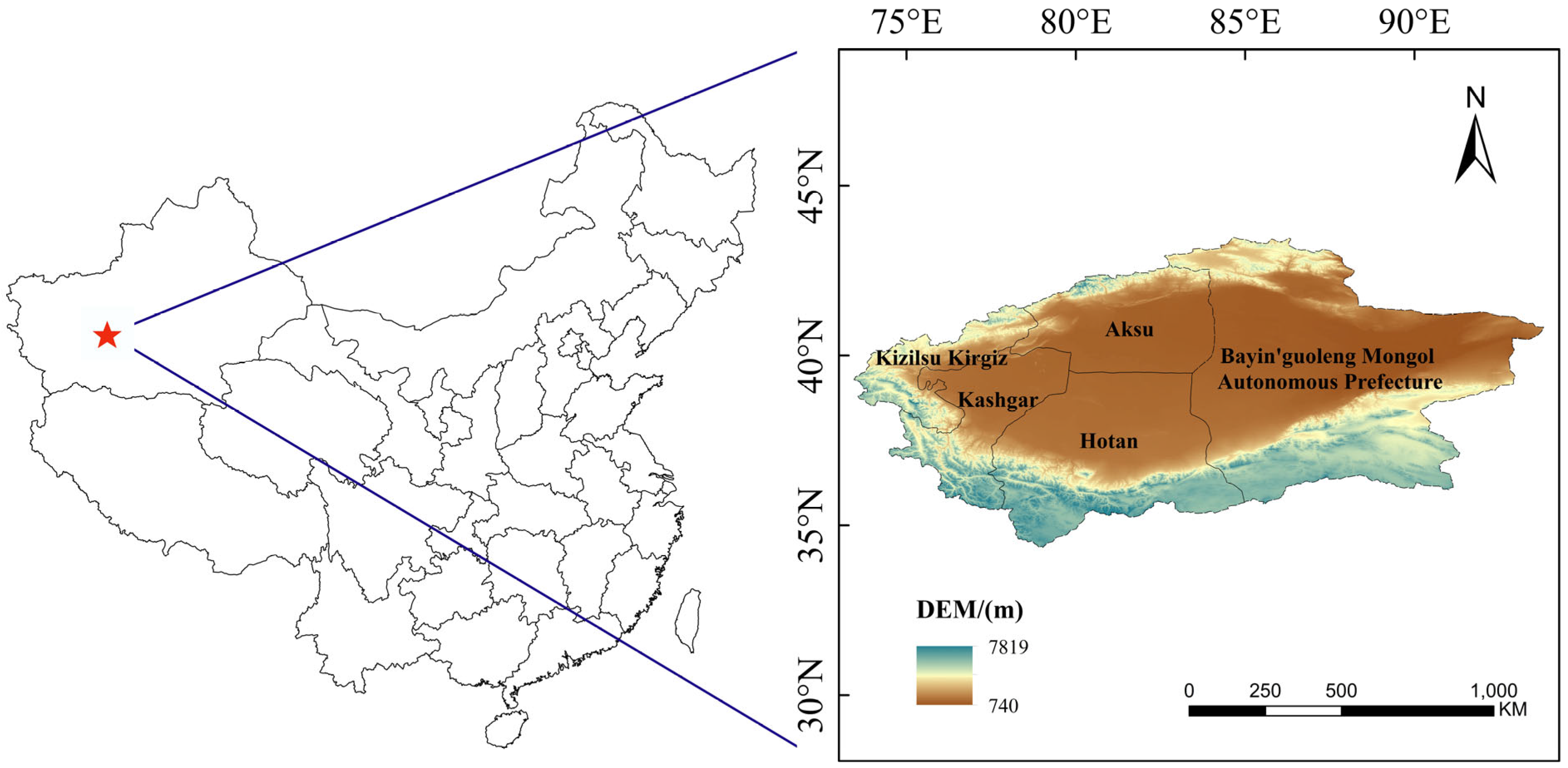
Xinjiang is the core region of the Silk Road Economic Belt, which has importance to the economic construction of the “Belt and Road” programme [23]. The unique geographical conditions of the southern border cause the atmosphere have different pollution characteristics and sources as well as different spatial structures and time changes [24]. In the hinterland of southern Xinjiang lies is the Taklamakan Desert, which is greatly affected by sand and dust. In the southern fringe of the desert and in the Hotan region, sand and dust storms are frequent in spring and summer [25,26,27]. Due to the unique characteristics of Xinjiang’s geographic conditions, atmospheric pollution characteristics, residents’ lifestyles, heating methods, and other reasons [28], the atmospheric environment has been damaged to a certain extent, directly or indirectly affecting Xinjiang’s development and its residents’ physical and mental health [29,30]. The region is less well-studied in terms of the characteristics of the spatial and temporal distribution of atmospheric PM_2.5 and O₃ concentrations in relation to typical precursors and particulate matter [31,32]. Therefore, this paper analyses and discusses five major aspects of the four air pollutants’ high-value areas and change characteristics, spatial autocorrelation, influencing factors, correlation between pollutants in the warm period, and impacts caused by air pollutants on human health in southern Xinjiang from 2018 to 2021 with a view towards providing a reference for future multi-pollutant synergistic studies, air pollution management, and the development of pollution control measures.

2. Overview of the Study Area

As shown in Figure 1, South Xinjiang is located in northwestern China. It lies south of the Tianshan Mountains and north of the Kunlun Mountains, roughly between latitudes 36° and 42° north and longitudes 73° and 86° east. In this paper, southern Xinjiang is divided into five regions according to administrative divisions: the Kizilsu Kirgiz, the Kashgar, the Aksu, the Hotan, and the Bayin’guoleng Mongol Autonomous Prefecture. The southern Xinjiang region has a typical temperate continental climate and the arid belt climate of Central Asia. Winters are long and cold, and summers are hot and dry. The average annual precipitation is lower than 50 mm, with abundant sunshine and large temperature differences. Southern Xinjiang accounts for 70% of the region’s forest and fruit cultivation. The Tarim Basin is China’s largest inland basin, occupying about 530,000 square kilometres. Its central part, the Taklamakan Desert, is the second-largest mobile desert in the world. This desert is also surrounded by oases such as the Tarim Oasis, the Celle Oasis (about 5333.3 km²), and the Andir Oasis (about 1187.3 km²), which are important ecosystems of irreplaceable significance to the local ecosystems and the lives of people [33]. The region is rich in coal and non-ferrous metals. The exploitation of mineral resources, the burning of coal and the full-scale promotion of new industrialisation have led to the destruction of the atmospheric environment while posing a serious threat to human health and the ecosystem.

3. Data Sources

The daily ozone tropospheric column concentration data, formaldehyde tropospheric column concentration data, and nitrogen dioxide tropospheric column concentration data used in this study were all obtained from the OMI (ozone monitoring instrument) on board the EOS-Aura satellite launched by NASA in the United States. The correlation between OMI satellite data and ground data has reached more than 0.82 [34,35]. The detector has a spatial resolution of 0.25° × 0.25°, a trajectory altitude of 705 km, and a wavelength range between 270 and 500 nm [36].

The PM_2.5 data are derived from the PM_2.5 dataset in the China High-Resolution High-Quality Near-Surface Air Pollutants (China High Air Pollutants, CHAP) dataset. The dataset uses artificial intelligence techniques to fill in the spatially missing values of the satellite MODIS MAIAC AOD product using modeled information. It combines ground-based observations, atmospheric reanalyses, and emission inventories with big data to obtain seamless national near-surface PM_2.5 data for the period from 2000 to 2021. The main scope is the entire region of China with a spatial resolution of 1 km and units of µg/m³.

Ground station O₃ and PM_2.5 data were provided by the National Urban Air Quality Real-Time Distribution Platform from the China Environmental Testing General Station, which is used to analyze the assessment of the health benefits of air pollutants on human beings.

Meteorological data were obtained from a dataset jointly provided by the National Centers for Environmental Prediction (NCEP) and the National Center for Atmospheric Research (NCAR) from the United States of America, which contains data from 1948 to the present.

4. Research Methodology and Data Processing

After obtaining the remote sensing data of daily ozone, formaldehyde, and nitrogen dioxide column concentrations in the study area from 2018–2021 and obtaining the data stored in the HDFEOS strip (swath) data format, the data were batch processed using VISAN3 and python programs. First, Python software was used to extract the latitude, longitude, pollutant column concentration, and cloudiness data; then, anomalies were excluded, and neighboring strip data were merged. PM_2.5 data were stored in the NC data format and were then converted to TIF in ArcGIS. Data files were formatted in ArcGIS. All pollutant data were re-sampled in ArcGIS and then converted into a format. Kriging spatial interpolation, averaging, and mask extraction were completed in order to obtain the spatial distribution map of pollutant concentration data in the southern Xinjiang region with an accuracy of 0.01 image elements.

4.1. Spatial Autocorrelation Analysis

Moran’s index is a classical method for calculating spatial autocorrelation [37] which is generally divided into two types: global spatial autocorrelation and local spatial autocorrelation [38]. The function of the global Moran’s I value is to describe the overall distributional aggregation of a phenomenon, and the formula for the global Moran’s I is as follows:

$$I=\frac{n{\displaystyle {\sum }_{i=1}^n{\displaystyle {\sum }_{j=1}^n{W}_{ij}\left(x_i-\overline{x}\right)}\left(x_j-\overline{x}\right)}}{{\displaystyle {\sum }_{i=1}^n{\displaystyle {\sum }_{j=1}^n{W}_{ij}{\displaystyle {\sum }_{i=1}^n{\left(x_i-\overline{x}\right)}^2}}}}\begin{array}{cc}& \left(i\ne j\right)\end{array}\begin{array}{cccc}& & \begin{array}{ccc}& & \end{array}& \end{array}$$

(1)

n represents the total number of samples, x_i is the observation of the variable at spatial unit i, and W_ij is the spatial neighbourhood weight matrix with $\overline{x}$ as its average. The Moran’s I index has a range of values between [−1, 1], with less than 0 indicating a negative correlation (a more spatially dispersed distribution). A value greater than 0 indicates a positive correlation (more aggregated spatial distribution). Equal to 0 indicates that the spatial object units are randomly distributed and spatially uncorrelated [39,40].

The local type Moran’s I is a spatial autocorrelation test statistic used to identify the location of spatial clusters and spatial outliers, and it is calculated as follows:

$$I_i=\frac{n\left(x_i-\overline{x}\right){\displaystyle \sum _{j=1}^n{W}_{ji}\left(x_j-\overline{x}\right)}}{{\displaystyle \sum _{i=1}^n{\left(x_i-\overline{x}\right)}^2}}$$

(2)

4.2. Geo-Temporally Weighted Regression Model (GTWR)

The geographically and temporally weighted regression (GTWR) model used in this paper was composed by Huang et al. [41] based on the spatial geographic weighted regression model and incorporates temporal characteristics into the model. It can comprehensively reflect the effects of the spatial location characteristics and temporal factors of the model. The GTWR model is a local linear regression model that takes into account spatio-temporal non-stationarity and represents a series of observations (Y₁, Y₂, …, Y_i) at the spatial location of (u_i, v_i) with the expression:

$$y={\beta }_0\left(u_i,v_i,t_i\right)+{\displaystyle \sum _{k=1}^P\beta \left(u_i,v_i,t_i\right)x_{ik}}+{\epsilon }_i\begin{array}{ccc}& i=1,2,3\dots ,n& \begin{array}{ccc}& & \end{array}\end{array}$$

(3)

where i = 1, 2, …, k, Y_i denotes the predicted concentration of each pollutant in the study area; β₀ denotes the intercept, β_1…k are the regression coefficients of the sample points (u_i, v_i, t_i), and ε_i denotes the residuals of the sample points (u_i, v_i, t_i). The final simulated values of the final model were plotted using the spline function method [42,43].

4.3. Pearson Correlation Analysis

In analyzing the spatial relationship between ozone, formaldehyde, and nitrogen dioxide concentrations and their relationship with natural factors (precipitation, temperature, and NDVI), this paper adopts Pearson correlation analysis. The correlation coefficient r reflects the positive or negative correlation between the variables and the strength of the correlation [44].

$$r_{\mathrm{xy}}=\frac{{{\displaystyle \sum }}_{i=1}^n\left[\left(x_i-\overline{x}\right)\left(y_i-\overline{y}\right)\right]}{\sqrt{{{\displaystyle \sum }}_{i=1}^n{\left(x_i-\overline{x}\right)}^2{{\displaystyle \sum }}_{i=1}^n{\left(x_i-\overline{y}\right)}^2}}$$

(4)

where: x and y represent two variables, r_xy is the correlation coefficient between the x and y variables, and i is the year number.

4.4. Spearman Correlation Analysis

In many studies, many data, whether natural factors, social factors, or pollutant concentrations, show non-linear trends. However, Spearman’s correlation can reflect the correlation between the trends of two non-linear elements. It is not necessary to ask whether the two elements are linear or not or whether they satisfy a normal distribution. Meanwhile spearman performs well in air pollutant correlation studies [45], so this paper uses spearman correlation to test the correlation of pollutant data. The calculation formula is as follows:

$$\begin{array}{c}{r}_s=1-\frac{6{\displaystyle \sum d_i^2}}{n\left(n^2-1\right)}\end{array}$$

(5)

$$\begin{array}{c}{d}_i=rg\left(X_i\right)-rg\left(Y_i\right)\end{array}$$

(6)

where n is the number of data and d_i is the difference between two data orders.

4.5. BenMAP-CE Model

The environmental benefit assessment model (BenMAP) is a geographic information system (GIS)-based model that estimates the health benefits associated with changes in air quality by creating population exposure surfaces in order to estimate changes in a range of health outcomes associated with air pollution [46]. BenMAP analyses the health effects of air pollution using a health impact function (HIF), which is shown below:

$$\mathsf{\Delta }Y=Y_0\left(1-e^{-\beta \mathsf{\Delta }X}\right)\times Pop$$

(7)

where $\mathsf{\Delta }$Y is the estimated health effect of the change in pollutant concentration, Y₀ is the baseline incidence of health endpoints (i.e., mortality or morbidity), Pop is the population affected by the change in air quality, $\mathsf{\Delta }$X is the change in air quality, and β is the coefficient of the relationship between the pollution concentration and the health effect (i.e., the coefficient of the exposure–response relationship) [47].

5. Results and Discussion

5.1. Characteristics of the Spatial Distribution of Multiple Pollutants

This paper processes and analyses O₃, NO₂, and HCHO column concentration data in the troposphere at 10–12 km altitudes and PM_2.5 concentration data at 1 km near the ground level in the South Xinjiang region for 2018–2021. The overall spatial distribution of the four-year annual mean values for the four pollutants was derived (Figure 2). Each indicator in the study area was classified into one of five classes according to the range of concentration values, from low to high values (blue to red bands), in order from the first to the fifth class.

As can be seen in Figure 2, the overall ozone concentration values show a decreasing distribution pattern from the southeast to the west and south of the country, with relatively low concentration values in the south of southern Xinjiang. Concentration values are at a high level overall, with high-value areas accounting for 62.8% of the southern Xinjiang area. They are mainly located in the eastern part of Kashgar, the southern part of Aksu, the northern part of Hotan, and the central part of the Bayin’guoleng Mongol Autonomous Prefecture.

The overall spatial distribution of the HCHO tropospheric column concentration is opposite to that of the ozone tropospheric column concentration. Its distribution is lower in the centre and increases step by step from the central desert area to the outside. The area with concentration values in the range of 8.5~11.5 × 10¹⁵ molec/cm² accounted for 65.8% of the study area. The high-value areas were distributed in the southern part of the Hotan area, the southern part of the Bayin’guoleng Mongol Autonomous Prefecture, and the northern region of southern Xinjiang. Since isoprene emitted by plants is the main component of VOCs, the contribution to the HCHO concentration was particularly prominent. Vegetation cover was significantly and positively correlated with HCHO concentrations [48], so the HCHO concentration values were higher in the northern part of southern Xinjiang than in the central and southern regions.

The distribution pattern of NO₂ tropospheric column concentrations shows a clear characteristic of latitudinal variation. Concentration values increased with increasing latitude, and the high-value areas were mainly distributed in the northeastern part of southern Xinjiang. The southeastern part of the Hotan area and the southern part of the Bayin’guoleng Mongol Autonomous Prefecture have lower concentration values, floating between 0.55~0.82 × 10¹⁵ molec/cm², which account for 33% of the area of southern Xinjiang. During China’s 13th Five-Year Plan economic policy development period, the centre of gravity of pollution in the cities of southern Xinjiang has continuously shifted from the northern part of the Hotan region to the Aksu region in the north–west direction [23]. Therefore, the area with high NO₂ concentration is concentrated in the northern part of southern Xinjiang.

The PM_2.5 concentration values as a whole show regular decreasing distribution characteristics. The high values are mainly concentrated in the central part of Hotan. Low-value areas are distributed at the border of the southern Xinjiang region and other regions. The hinterland of southern Xinjiang is the Tarim Basin, which contains the Taklamakan Desert, with high temperatures and little rainfall all year round. Sand and dust pollution is the main force of air pollution in southern Xinjiang, and the contribution of desert dust to PM_2.5 is quite obvious. Due to the special geographical conditions, pollutants are very difficult to spread. The prolonged wandering and accumulation in the basin results in higher PM_2.5 concentrations here than in other areas.

5.2. Characteristics of Monthly Variations in Multi-Pollutant Concentrations

In order to analyse the characteristics of monthly changes in pollutants in the southern border area, monthly average concentration level stacking charts and monthly average time change line charts of four pollutants were made.

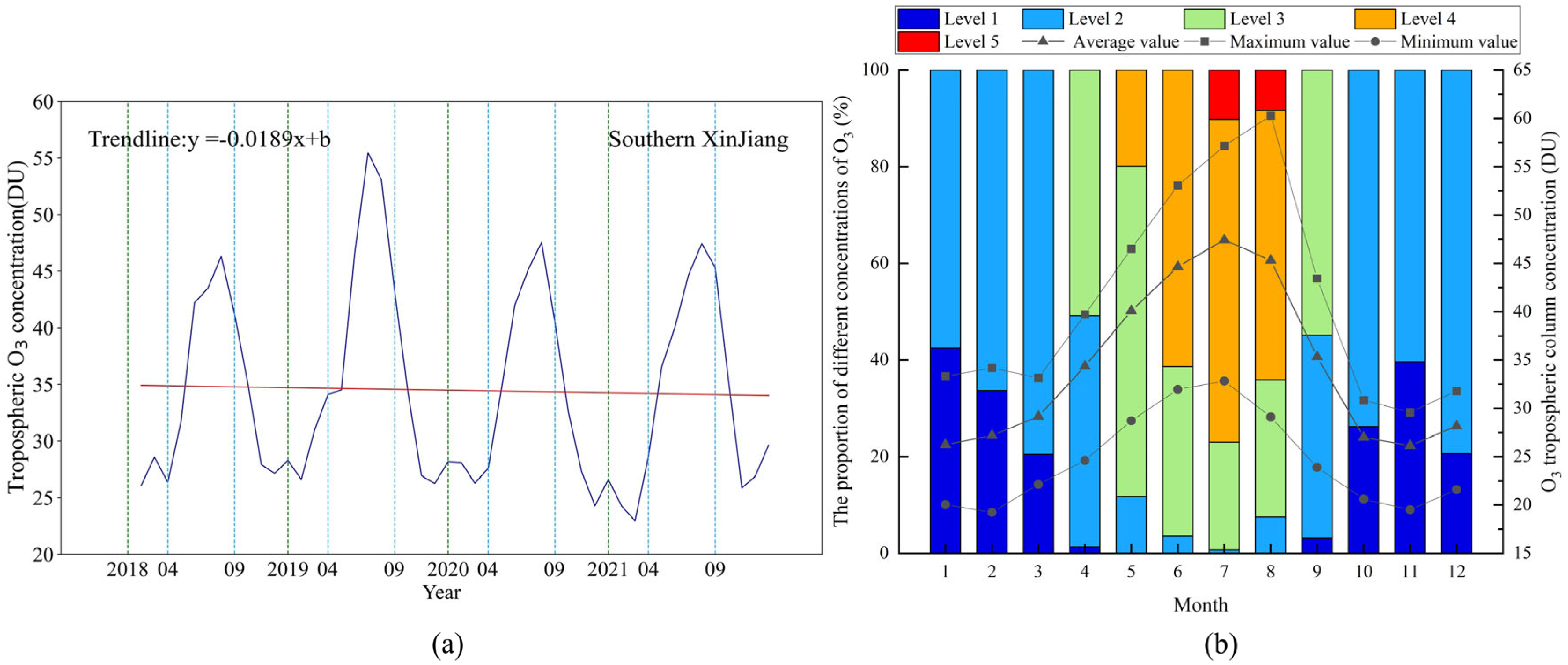
5.2.1. Characteristics of Monthly Changes in Tropospheric Ozone Column Concentrations

Figure 3 shows the monthly average rank stacking and time variation of ozone over four years with the monthly average stacking divided into five classes (Class 1: 17~26 DU, Class 2: 26~35 DU, Class 3: 35~44 DU, Class 4: 44~53 DU, and Class 5: 53~62 DU). As shown in the figure, the tropospheric ozone column concentration in the southern Xinjiang region shows a unimodal cyclic pattern of change. The obvious high value area from April to September is the warm period. During the warm period, the ozone column concentration peaked (47.43 DU), and the maximum value rose by 4.089 DU in the month. Fitting the mean values of all the months, a fitted line was obtained, and the slope of the fit was −0.0189. This indicates a slight downward trend in ozone concentrations. The four-year concentration maximum and minimum values appeared in June 2019 and February 2021, with concentration values of 65.36 DU and 15.43 DU, respectively.

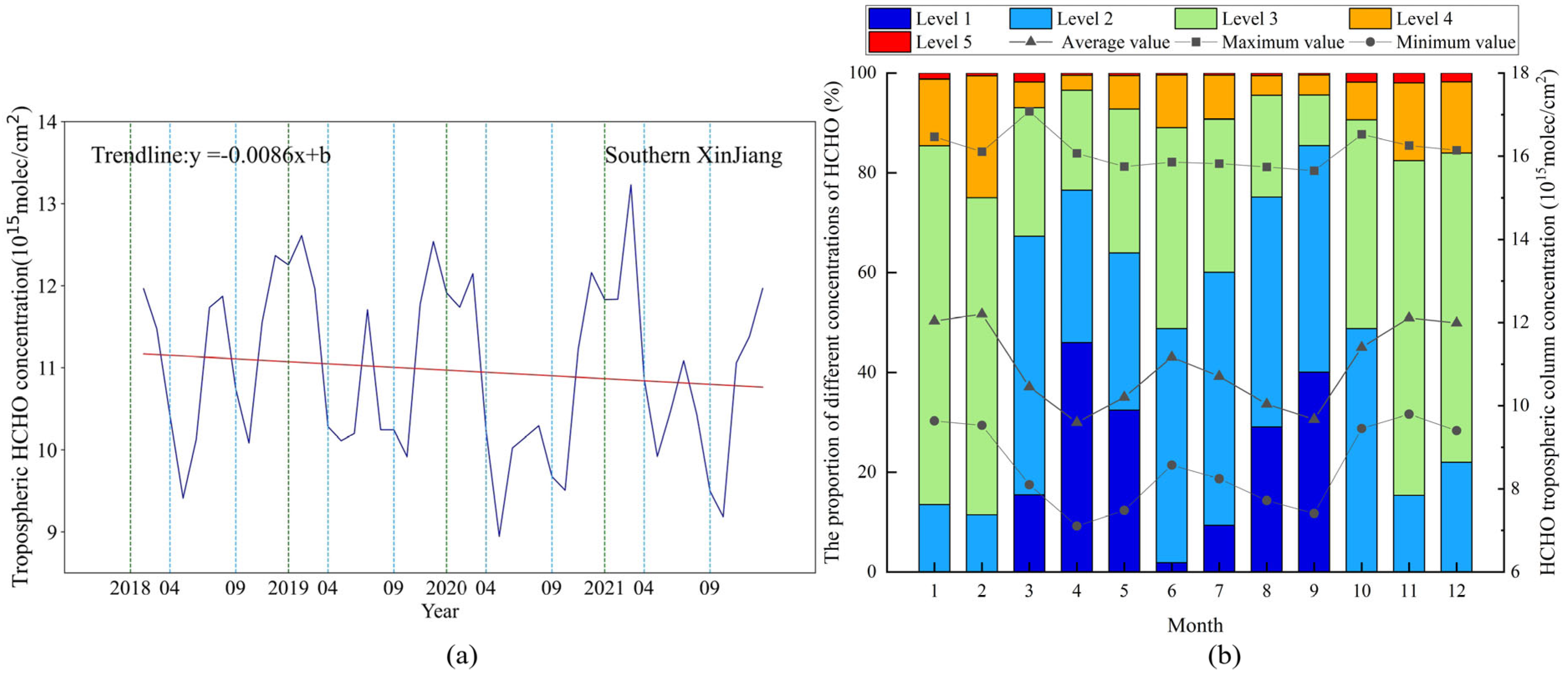
5.2.2. Characteristics of Monthly Changes in Tropospheric Formaldehyde Column Concentrations

As shown in Figure 4, the HCHO concentration values in the southern Xinjiang region were comparable to those in the Yangtze River Delta region [49]. The stacked graph of the four-year monthly average HCHO column concentrations was classified into five classes (Class 1: 6.8 × 10¹⁵~8.9 × 10¹⁵ molec/cm², Class 2: 8.9 × 10¹⁵~11 × 10¹⁵ molec/cm², Class 3: 11 × 10¹⁵~13.1 × 10¹⁵ molec/cm², Class 4: 13.1 × 10¹⁵~15.2 × 10¹⁵ molec/cm², and Class 5: 15.2 × 10¹⁵~17.3 × 10¹⁵ molec/cm²). In the stacking diagram, the monthly average concentration values showed a significant decreasing trend in March (decreasing rate of 14.36%) with a slight increase in June, but they were overall mainly in Class 1–2 in the following six months (accounting for 48.78~85.47% of the overall area).The highest value occurred in February with 12.2 × 10¹⁵ molec/cm² and the lowest in April with 9.6 × 10¹⁵ molec/cm². The difference between the maximum and minimum values was 4.28 × 10¹⁵ molec/cm² over the four years. Fitting the mean values for all of the months revealed a slow decreasing trend, with the slope of the fitted line being −0.0086 with slow downward trend. The mean values of the tropospheric HCHO column concentrations over the monthly time variations were 10.97 × 10¹⁵ molec/cm² up and down. Overall, monthly average HCHO concentration values showed a double-trough pattern of change, reaching the size of the trough in April and September, with a range of 0.195 × 10¹⁵~0.735 × 10¹⁵ molec/cm².

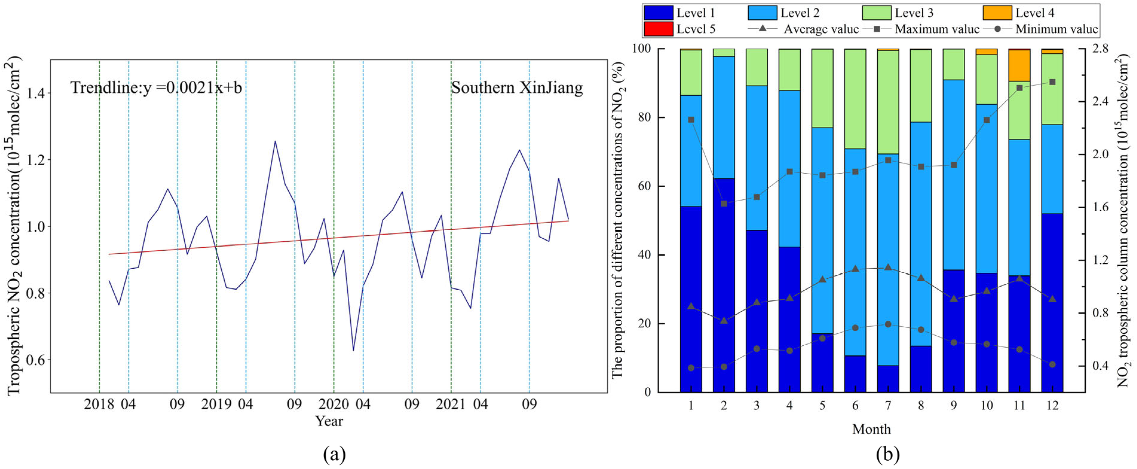
5.2.3. Characteristics of Monthly Variations in Column Concentrations of Nitrogen Dioxide in the Troposphere

Figure 5 shows the four-year monthly average rank pile-up and time variation of nitrogen dioxide, which was classified into five levels (Level 1: 0.37 × 10¹⁵~0.81 × 10¹⁵ molec/cm², Level 2: 0.81 × 10¹⁵~1.25 × 10¹⁵ molec/cm², Level 3: 1.25 × 10¹⁵~1.69 × 10¹⁵ molec/cm², Level 4: 1.69 × 10¹⁵~2.13 × 10¹⁵ molec/cm², and Level 5: 2.13 × 10¹⁵~2.57 × 10¹⁵ molec/cm²). According to the monthly average stacking map, the overall nitrogen dioxide concentration was low without obvious extreme pollution, dominated by Levels 1 and 2, which accounted for 69.36~97.74% of the total area. The monthly mean concentration value was highest in July at 1.14 × 10¹⁵ molec/cm² and lowest in February at 0.74 × 10¹⁵ molec/cm². In the month-by-month time-varying graph, the overall trend showed a double-peak pattern, with a maximum peak in July and a smaller peak in November, with a maximum–minimum difference of 0.23 × 10¹⁵ molec/cm². Fitting the monthly average concentration values reveals that the nitrogen dioxide concentration values have slowly increased in recent years.

5.2.4. Characteristics of Monthly Changes in PM_2.5 Concentrations

The four-year monthly average rank stacking map and time variation of PM_2.5 are shown in Figure 6, which divides the monthly average stacking map into five classes (Class 1: 10~48 µg/m³, Class 2: 48~86 µg/m³, Class 3: 86~124 µg/m³, Class 4: 124~162 µg/m³, and Class 5: 162~200 µg/m³). From Figure 6, it can be seen that the PM_2.5 concentration was significantly higher in March–May than in other months, with Class 3–5 accounting for 40.3~51.5% of the overall area. Dusty weather is active from March to August, with May to August being the most severe period. The average number of dusty days per month is nearly 15, exceeding the annual average by 30%. March is the month when the maximum PM_2.5 concentration is more concentrated. The maximum and minimum difference is 45.37 µg/m³. The monthly time changes show that in 2018 and 2020, there is a double-peak trend, with more significant peaks in March and April and smaller peaks in September. Concentration values fluctuated significantly in 2019 and 2021, with a maximum difference of 60.08 µg/m³ between peaks. The overall trend of concentration values during the study period was slowly decreasing, with a fitted slope of −0.2569.

5.3. Spatial Autocorrelation Characteristics of Multiple Pollutants

The global spatial autocorrelation characteristics of O₃, NO₂, HCHO, and PM_2.5 concentrations in the southern Xinjiang region from 2018 to 2021 were analyzed using ArcGIS spatial statistical tools based on Moran’s I index. The spatial relationship conceptualization was adopted as INVERSE_DISTANCE to test whether there is any aggregation of the concentrations of each pollutant in the southern Xinjiang region.

In this subsection, spatial autocorrelation and local autocorrelation were studied for each of the four pollutants, and Moran’s I index reflects whether there is spatial correlation for the four pollutants as well as the positive and negative correlation. The Z value is the standard deviation multiplier, which is used to reflect the degree of dispersion of the distribution of pollutant concentration values, and it shows an aggregated distribution when Z > 1.65. In the local autocorrelation, H-H clusters represent areas of high concentration and high values in the surrounding area, while L-L clusters represent areas of low concentration both in the region and in the surrounding area.

The analysis of the spatial autocorrelation of the concentration of each pollutant during the four years found that the p-values generated by the four pollutants were less than the significant level of 0.01, with a confidence level of 99%; in

Table 1. Moran’s I values and Z scores for year-by-year and four-year average concentrations of four pollutants, 2018–2021.

	O3		NO2		HCHO		PM2.5
Time	I	Z	I	Z	I	Z	I	Z
2018	0.975	140.966	0.993	143.292	0.987	142.708	0.984	142.266
2019	0.976	141.026	0.994	143.549	0.988	142.740	0.983	142.113
2020	0.976	141.079	0.995	143.594	0.987	142.702	0.985	142.392
2021	0.977	141.207	0.997	143.986	0.986	142.265	0.986	142.629
4 year average	0.976	141.067	0.995	143.614	0.987	142.432	0.985	142.416

, the Z scores exceeded the critical value of 2.58, and the values of each pollutant’s I-value were all greater than 0.5, indicating that the distribution of each pollutant’s spatial concentration in the southern border region presents a significant agglomeration effect. Changes in Z scores and I values indicate that there is some volatility in the magnitude of spatial agglomeration. From the I value and Z score of each pollutant across four years, O₃ and NO₂ aggregation both showed a slow increasing trend, with an average annual increase of 0.068% and 0.134%, respectively. HCHO continues to decline after a small rebound in 2019. The average annual decline is 0.034%. PM_2.5 changes inversely with HCHO aggregation. It shows an upward trend after a small decrease in 2019, with an average annual increase of 0.068%. From the above, it can be seen that the aggregation of O₃, NO₂, and PM_2.5 shows an upward trend in the region. This indicates that the spatial aggregation effect is increasing year by year, and there is a small decrease in the level of air quality. The decrease in the aggregation of HCHO also reflects that the vegetation in the southern border area has been damaged to a certain extent, and the ecological quality of the vegetation has declined.

Since there are no significant fluctuations in the I value and Z score of each pollutant in four years, the annual average values of 2018–2021 are used to analyze the local spatial autocorrelation of the concentration of each pollutant. Figure 7 shows that the L-L concentration of the four-year annual mean O₃ concentration in the southern Xinjiang region mainly occurs in the southern part of the southern Xinjiang region, while the H-H concentration mainly occurs in the northeastern part of the Hotan region, the southeastern part of the Aksu region, and the central part of the Bayin’guoleng Mongol Autonomous Prefecture, which shows a spatial positive correlation characteristic with significant spatial dependence; the H-H concentration also exists in a small part of the northeastern area of the Kashgar region. The spatial dependence of annual mean HCHO concentrations was significantly positively correlated in the area bordering the northern part of the southern border with the southern part of northern Xinjiang, the southern part of Hotan, and the southern part of the Bayin’guoleng Mongol Autonomous Prefecture. The L-L concentration area overlaps with the H-H concentration area of O₃ located in southern Xinjiang’s central area. The L-L concentration of the annual mean concentration of NO₂ mainly occurs in the southeastern region of the southern border since the industrial zones are concentrated in the northern part of the Aksu and Yuliu counties—the northern region—while H-H aggregation occurs in the northern region of southern Xinjiang. The H-H aggregation of annual mean PM_2.5 concentration occurs in the hinterland region of southern Xinjiang, i.e., near the Tarim Basin. Wind, as one of the main driving forces of air pollution, may be due to the formation of a cyclonic flow field in the basin as a result of the topography, which creates a “stagnation zone” within the southern hinterland [50]. The L-L agglomeration area is located around the border in southern Xinjiang.

5.4. Analysis of Influencing Factors Based on the GTWR Model

Geographical and temporal weighted regression (GTWR) can effectively solve the issue of spatial and temporal non-stationarity of spatial data [51,52], which can take into account the effects of time and location. In this paper, the five influencing factors and the four-year month-by-month average concentration values of each pollutant were selected. The GTWR model was used to test the spatio-temporal heterogeneity between the two (data were not de-seasonalised). At the same time, there is a multilinear regression relationship between the pollutants and the influencing factors. In this paper, the selected data have been standardised in order to remove the effect of multicollinearity on the analysis results. In most studies, people mainly choose temperature, precipitable water, and air pressure to analyse the influence of natural factors on air pollutants. Since the hinterland area of southern Xinjiang is the Taklamakan Desert, and the regional boundaries of the distribution of vegetation cover are more obvious, this paper adds the influence of NDVI on the four pollutants.

In this paper, PER (precipitable water, the total amount of water vapour contained in the atmospheric column per unit area), TEM (temperature), PS (atmospheric pressure), RH (relative humidity), and NDVI (normalized vegetation index) were selected to analyze the regression coefficients of influencing factors with the four pollutants, respectively.

As can be seen from

Table 2. Regression coefficients and R² of pollutants and influencing factors in geographic and temporal weighted regression models, 2018–2021.

Variables	R2	Min.	Max.	Average	Standard Deviation
O3-PER	0.860	−2.654	3.056	0.457	0.62
O3-TEM		−9.2	8.445	0.835	1.63
O3-PS		−11.737	6.966	−0.89	1.81
O3-RH		−2.275	2.882	0.154	0.62
O3-NDVI		−2.962	2.449	−0.036	0.38
NO2-PER	0.856	−1.83	2.84	0.141	0.53
NO2-TEM		−3.669	6.679	0.54	1.06
NO2-PS		−5.837	14.279	0.691	1.96
NO2-RH		−2.611	2.855	0.182	0.57
NO2-NDVI		−3.213	3.931	0.29	0.45
HCHO-PER	0.638	−3.062	4.165	−0.149	1.04
HCHO-TEM		−7.4	7.777	−0.631	1.74
HCHO-PS		−6.323	21.6	1.34	3.37
HCHO-RH		−2.764	4.514	0.241	0.75
HCHO-NDVI		−3.9	7.322	0.305	0.61
PM2.5-PER	0.678	−4.595	3.9	0.19	1.05
PM2.5-TEM		−7.576	7.904	−0.01	1.96
PM2.5-PS		−28.889	12.353	−0.626	4.75
PM2.5-RH		−4.994	3.404	0.009	0.77
PM2.5-NDVI		−5.22	5.935	−0.422	0.86

, the R² of each indicator in the GTWR model for 2018–2021 is more significant than 0.6, with a good fit. As can be seen from the analysis in Table 2 and Figure 8, air temperature, precipitable water, and relative humidity were positively correlated with O₃. Air temperature has the strongest positive correlation, with a mean regression coefficient of 0.835. The negative correlation between atmospheric pressure and O₃ is high. The regression coefficient reached −0.89. In the northeastern part of the Aksu region, the central-eastern part of the Hotan region, and the southwestern part of the Bayin’guoleng Mongol Autonomous Prefecture, the precipitable amount of precipitation showed a strong positive correlation with ozone. The correlation coefficients ranged from 0.49 to 1.77. As the mid-latitude westerly wind belt controls the southern Xinjiang region, its geographical latitude, topographic height, and atmospheric circulation result in higher atmospheric precipitable water in the basin area. When the Central Asian low vortex occurs, the atmospheric precipitable water in the Tarim Basin is higher than in the areas distributed along the mountain ranges [53,54]. The areas of positive temperature and ozone correlation are located in the westernmost and southernmost parts of southern Xinjiang. The ozone concentration values in this region are low. As the region is located at the southern edge of the Tarim Basin, it is a special topography surrounded by mountains on three sides and open to the east. The resultant centres of low-temperature values are also mainly located in the southern part of southern Xinjiang [23]. Atmospheric pressure was predominantly negatively correlated with ozone in southern Xinjiang’s northwestern and eastern parts. It has a greater impact on the easternmost part of the Bayin’guoleng Mongol Autonomous Prefecture, with correlation coefficients fluctuating from 3.04 to 5.85.

There is a significant correlation between airborne NOx content and the duration of presence and temperature [48]. All five influencing factors showed predominantly positive correlations with NO₂ concentrations. Among them, atmospheric pressure has a stronger influence, followed by air temperature. The positively correlated areas accounted for 58.17% and 85.22% of the overall area, respectively. In the southwestern and northeastern parts of southern Xinjiang, the correlation coefficients between atmospheric pressure and NO₂ concentration were as high as 5.92–10.62. The area of the positive correlation region gradually decreased towards the central part of southern Xinjiang. Temperature has a greater effect on NO₂ concentrations in the northern and southwestern parts of southern Xinjiang.

The influences with strong correlation with HCHO were temperature, atmospheric pressure, and NDVI. Their correlation coefficients were −0.631, 1.34, and 0.305, respectively. The area of negative correlation between temperature and HCHO concentration accounts for 98.94% of the overall area. The northern and southwestern regions of the southern Xinjiang had a greater effect of temperature on HCHO concentration. The temperature in southern Xinjiang is high compared to northern Xinjiang. The Taklamakan Desert is located in the hinterland of southern Xinjiang, with high temperatures and little rainfall all year round. Excessively high temperatures lead to reduced mycorrhizal activity in the roots of vegetation, closure of stomatal channels, and inhibition of isoprene production, thus shortening the survival time of HCHO [49]. Atmospheric pressure has a strong positive correlation with HCHO in the northern part of southern Xinjiang. The strongest correlations between NDVI and HCHO concentrations were found in the northwestern and eastern parts of the Kizilsu Kirgiz Autonomous Prefecture and the southeastern part of the Hotan region. The Hotan region has a high forest cover of 6.8% and a grass cover of 30.3%. This indicates that the region is under conditions favourable for formaldehyde release all year round, so the positive correlation is strong [49].

The factors that were more strongly correlated with PM_2.5 were atmospheric pressure and NDVI, and both were negatively correlated. Atmospheric pressure has a stronger negative correlation compared to NDVI. It is distributed in the southwestern and southeastern parts of the study area, accounting for 79.48% of the overall area. The area of negative correlation between NDVI and PM_2.5 is mainly distributed in the southern and northwestern parts of southern Xinjiang, with correlation coefficients ranging from −1.19 to −0.12. Although vegetation’s blocking and absorbing effect has a positive impact on the removal of atmospheric particulate matter PM_2.5, the retention of too much atmospheric particulate matter can have a negative effect on plant growth [55].

5.5. Warm Period Multi-Pollutant Correlation Analyses

Many studies have looked more at the relationship between pollutants and natural and social factors, and fewer at the interactions between pollutants. Pollutant monitoring in China divides atmospheric pollutants into six major pollutants that are monitored individually. Although some of these pollutants are correlated (e.g., NO₂ and O₃) there is little research on this topic in the Chinese region. At the same time, the southern border region has special geographical conditions and is more affected by sand and dust. The interactions between pollutants and the magnitude of their contributions to each other are different from those in other regions. Therefore, conducting two-by-two correlation studies and partial correlation analyses of pollutants in multi-pollutant studies in this paper for the southern Xinjiang region is necessary. In turn, the extent to which they are affected by other pollutants is explored in a comparative manner.

From the above study, it can be determined that the ozone concentration values from April to September (warm period) appear as a significantly high-value area throughout the year. As ozone precursors, the contribution of NO₂ and HCHO to ozone should be explored separately for this period. There are small peaks in PM_2.5 concentration changes during the warm period. Changes in the concentration of dust particles in the desert can impact vegetation, which in turn alters the production of HCHO and O₃. Therefore, this paper also explores the impact and relevance of changes in the concentration of dust particulate matter (represented by PM_2.5) on other air pollutants. In order to provide a reference for inter-pollutant correlation studies and atmospheric management in the more severe dusty areas.

5.5.1. Interrelationships between Pollutants in the Southern Border Region

The monthly mean concentration values of O₃, NO₂, HCHO, and PM_2.5 from April to September 2018–2021 (warm period) were tested for normal distribution among each other. Pearson’s correlation analysis was conducted among the concentration values that satisfied the normal distribution. Spearman’s correlation analysis was carried out among the concentration values that did not satisfy the normal distribution.

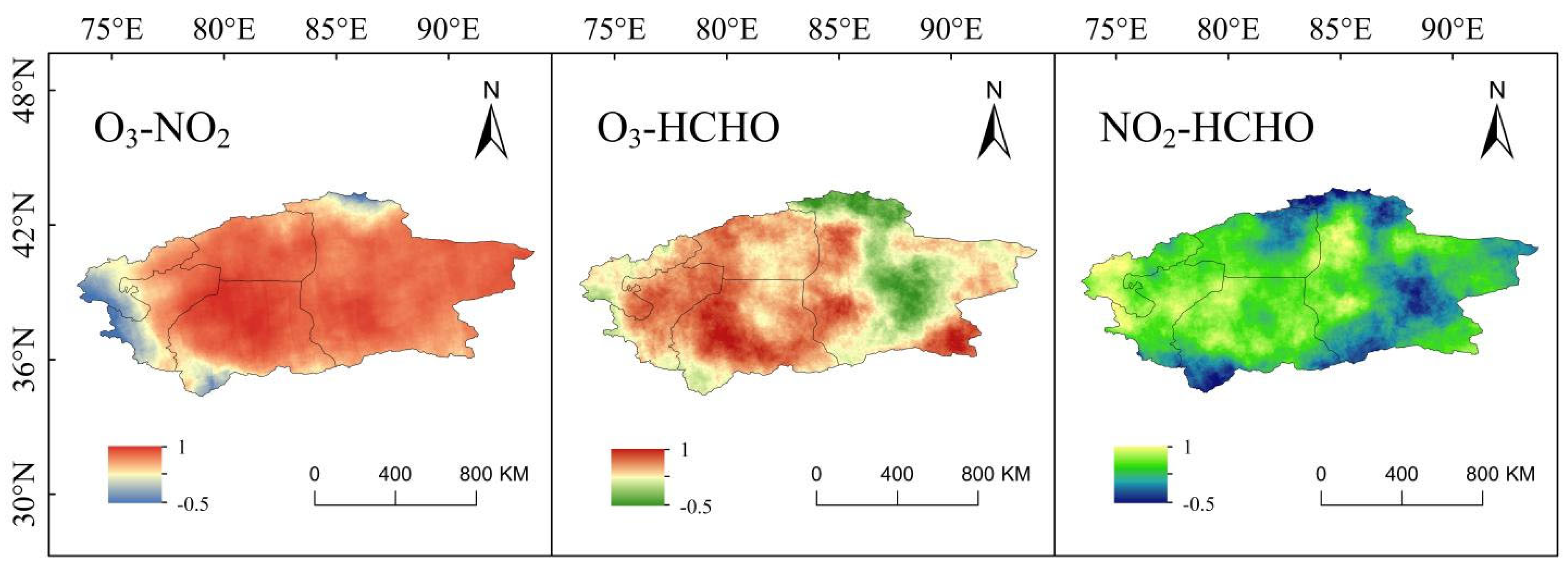
Figure 9 shows the spatial distribution of Pearson correlation between pollutants, and the results show that 99.8% of the area between O₃ and NO₂ is positively correlated. The mean value of the correlation coefficient is 0.746. Negative correlation areas are distributed in the north and southwest of southern Xinjiang. Industry (coal industry, etc.) is mainly concentrated in the northern part of southern Xinjiang. The combustion of coal produces large amounts of NO. NO is exposed to the air and then converted to NO₂, which accumulates in the air [48]. O₃ showed positive correlation with HCHO. The mean value of the correlation coefficient was 0.436, and the positive correlation area accounted for 98.7% of the total study area. The negative correlation areas are concentrated in the northern and central parts of the Bayin’guoleng Mongol Autonomous Prefecture. NO₂ and HCHO are precursors of ozone. The mean value of the correlation coefficient between the two was 0.431. Positive correlations were shown in the Kizilsu Kirgiz Autonomous Prefecture, the Kashgar Region, the north-central part of the Hotan Region, and the western and far-eastern parts of the Bayin’guoleng Mongol Autonomous Prefecture. The relationship between ozone and the photochemical reaction concentrations of NO_X and VOC_S is not a simple linear dependence but rather a nonlinear dependence [56], which affects the photochemical production of ozone when the concentration ratio of NO_X and VOC_S is relatively moderate [57,58]. From the above analyses, it can be seen that NO₂ contributes more to O₃ production than HCHO. Both complement each other and synergistically influence the change in O₃ concentration.

Figure 10 shows the spatial distribution of Spearman’s correlation among pollutants and the areas where the correlation between O₃ and PM_2.5, NO₂ and PM_2.5, and HCHO and PM_2.5 passed the 95% confidence test, which accounted for 34.42%, 44.24%, and 31.67%, respectively, of the total study area. The areas where the correlation between O₃ and PM_2.5 passed the confidence test were concentrated in the Kizilsu Kirgiz Autonomous Prefecture, northern Kashgar, north-central Aksu, and northern Bayin’guoleng Mongol Autonomous Prefecture, with a significant negative correlation and a correlation coefficient as high as −0.7872. The areas where the correlation between NO₂ and PM_2.5 passed the confidence test are located in the eastern part of the Aksu region and east-central Bayin’guoleng Mongol Autonomous Prefecture, with 99.97% of the areas having a high negative correlation and a correlation coefficient as high as −0.5427. The correlation between HCHO and PM_2.5 is mainly negative. The positive correlation area only accounts for 10.22% of the tested area, and the distribution is very scattered. The mean value of the correlation coefficient of the tested area is −0.4194. Hostile correlation areas are concentrated in the areas with low values of HCHO concentration: the northeastern part of Kashgar, the southern part of Aksu, the southern part of Hotan, and the central part of the Bayin’guoleng Mongol Autonomous Prefecture. From the correlation analysis, it can be seen that O₃ is strongly influenced by PM_2.5, and PM_2.5 contributes relatively little to the production of HCHO and NO₂.

5.5.2. Partial Correlation between Multi-Pollutants in the Southern Border Region

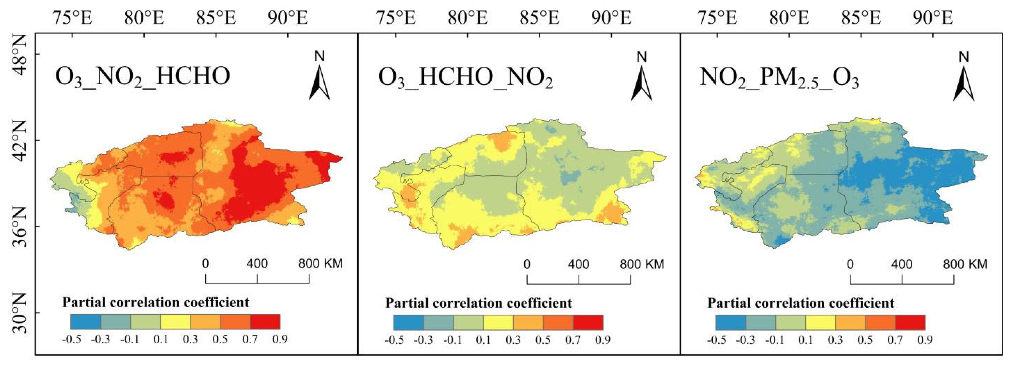
From the above correlation analysis, it can be seen that O₃ is strongly correlated with NO₂ and HCHO, respectively, and NO₂ is strongly correlated with PM_2.5. In order to exclude the interference of other pollutants on their correlations, a partial correlation analysis was carried out between the above pollutants, as shown in Figure 11. When the influence of HCHO is excluded, the correlation coefficients between O₃ and NO₂ are between (−0.219~0.875). The correlation coefficient decreased by 0.2063 compared to that in the Pearson correlation analysis. The positive correlation area accounted for 97.57% of the study area, and the correlation was more pronounced in the eastern and south-central regions of the Bayin’guoleng Mongol Autonomous Prefecture. Low negative correlations were found in the southeastern Kizilsu Kirgiz Autonomous Prefecture and a small area of the western part of the Kashgar region. When NO₂ is excluded, the correlation between O₃ and HCHO changed from a moderate positive correlation to a low positive correlation. The mean value of the correlation coefficient decreased by 0.3234. In the central region, where ozone is higher, a low-to-moderate negative correlation dominates. Many coal enterprises are concentrated in the southern Xinjiang region, emitting NO_X and PM_2.5. NO_X affects the concentration of O₃ under certain conditions, so the effect of O₃ is excluded in order to explore the correlation between NO₂ and PM_2.5. Among them, 85.04% of the regions were negatively correlated. The central and eastern regions of the Bayin’guoleng Mongol Autonomous Prefecture were moderately negatively correlated. The areas of positive correlation are all low positive correlation and are more dispersed in distribution.

In summary, there is a stronger correlation between O₃ and NO₂ compared to HCHO. The correlation between O₃ and HCHO is more affected by NO₂ in the southern part of the Aksu region and the northern part of the Hotan region. The mean value of the correlation coefficient between NO₂ and PM_2.5 increased by 0.3765 after excluding the effect of O₃. The correlation changed from a medium-high negative correlation to a low negative correlation. The southeastern part of the Hotan region is more affected by O₃. It is concluded that when O₃ is affected by both HCHO and NO₂, NO₂ interferes more with the correlation between O₃ and HCHO. At the same time, the various pollutants interact and reinforce each other. One pollutant is transformed into a precursor of another pollutant under certain conditions, causing its concentration value in the atmosphere to fluctuate accordingly. This ultimately leads to changes in air quality.

5.6. Assessment of Health Benefits from Pollutant Exposure

Air quality is inextricably linked to human health, and air pollution, especially PM_2.5 and O₃ pollution, has brought huge health impacts and economic losses to China. Therefore, this paper selects the above two pollutants to evaluate their health benefits.

The pollutant data for the health effects assessment in this paper are taken from pollutant ground station data based on data from the Xinjiang Regional Statistical Yearbook. Only the health effects due to O₃ and PM_2.5 pollution are explored here for 2018–2020 in four regions. This paper analyses the effects of three diseases on premature human mortality aggregated across regional spatial scales. The health effects in different regions, shaped by differences in the spatial distribution of pollutant concentrations and population sizes, are explored. For each health assessment outcome, random sampling was performed from the probability distribution of each exposure–response coefficient using the BenMap-CE model, and then the incidence rate was calculated based on the selected values [59,60,61] and the air quality standards [16,62] were used to calculate the incidence rates. The exposure–response coefficients for each health endpoint in the above four regions are shown in

Table 3. Range of exposure-response coefficients β for O₃, PM_2.5 exposure leading to all-cause premature death, premature death from cardiovascular disease, and premature death from respiratory disease.

Pollutant	Health Impact	Max-β	Mean-β	Min-β
O3	All-cause premature death	0.0035	0.0024	0.0013
	Premature death from cardiovascular disease	0.0044	0.0027	0.001
	Premature death from respiratory disease	0.0097	0.0073	0.0049
PM2.5	All-cause premature death	0.00504	0.00296	0.000896
	Premature death from cardiovascular disease	0.00093	0.00068	0.00053
	Premature death from respiratory disease	0.00221	0.00109	0.00143

. O₃ and PM_2.5 are more polluted in the Hotan and Aksu regions. This study also compared the changing relationship between the two air pollutants and the number of premature deaths in these two regions, as shown in

Table 4. Rates of change in pollutant concentrations and premature deaths in the Hotan and Aksu regions, 2018–2020.

Pollutant	Region	Year	Rate of Change of Pollutant Concentration Values	Rate of Change in All-Cause Premature Deaths	Rate of Change in Premature Deaths from Cardiovascular Disease	Rate of Change in Premature Deaths from Respiratory Diseases
O3	Hotan	2018–2019	+2.55%	+4.24%	+4.3%	−0.276%
		2019–2020	+9.85%	+22.46%	+25.83%	+1.39%
	Aksu	2018–2019	−2.92%	−7.14%	−6.95%	−10.52%
		2019–2020	−4.04%	+1.23%	+3.99%	−14.41%
PM2.5	Hotan	2018–2019	−10.03%	−20.79%	−20.77%	−23.86%
		2019–2020	+35.92%	+76.8%	+83.56%	+47.76%
	Aksu	2018–2019	−24.68%	−49.78%	−50%	−52.27%
		2019–2020	+13.47%	+95.61%	+102.86%	+66.67%

.

5.6.1. Health Benefits Assessment of Ozone Pollution

Table 5. Range and mean value of the number of people whose health is affected under the O₃ exposure scenario, 2018–2020 (10,000 people).

Year	District	All-Cause Premature Death	Premature Death from Cardiovascular Disease	Premature Death from Respiratory Disease
2018	Kizilsu Kirgiz	478 (267~677)	277 (107~433)	157 (112~197)
	Aksu	1484 (821~2117)	863 (330~1360)	504 (354~639)
	Hotan	1038 (571~1492)	605 (229~963)	362 (251~466)
	Kashgar	2810 (1557~4006)	1633 (627~2571)	949 (669~1203)
2019	Kizilsu Kirgiz	392 (217~558)	228 (88~359)	126 (89~160)
	Aksu	1378 (761~1969)	803 (307~1270)	451 (316~575)
	Hotan	1082 (595~1553)	631 (240~1004)	361 (251~464)
	Kashgar	2685 (1486~3832)	1565 (599~2467)	874 (614~1109)
2020	Kizilsu Kirgiz	334 (184~477)	200 (76~316)	92 (64~117)
	Aksu	1395 (770~1996)	835 (319~1323)	386 (270~494)
	Hotan	1325 (732~1896)	794 (303~1256)	366 (256~467)
	Kashgar	2437 (1346~3484)	1459 (557~2306)	672 (471~856)

shows the number of premature deaths from different diseases due to O₃ pollution in the four regions in 2018–2020. The number of premature deaths showed an overall decreasing trend year by year in the Kizilsu Kirgiz Autonomous Prefecture and the Kashgar region. The number of premature deaths in the Aksu region showed a decreasing trend in 2018–2019 and a slight increase in 2020. The number of premature deaths due to all-cause premature deaths and cardiovascular diseases in the Hotan region has been on the rise for three years. The number of premature deaths due to respiratory diseases showed a decreasing and then an increasing trend. Overall, the number of premature deaths due to O₃ pollution was highest in the Kashgar region followed by the Aksu and Hotan regions. The number of premature deaths from cardiovascular diseases was higher than that from respiratory diseases.

In 2020 compared to 2018, the Kizilsu Kirgiz Autonomous Prefecture had the largest decrease in premature deaths due to respiratory diseases, at 41.4%. The Aksu region showed the smallest decline in the number of premature deaths from cardiovascular diseases, at 3.24%. Unlike the remaining three regions, the number of premature deaths from the three diseases in Hotan is on the rise. As can be seen from Table 4 and Table 5, the trends in the number of premature deaths from the three diseases in 2018–2020 are basically consistent with the trends in ozone concentration. This shows that there is a direct impact of ozone pollution on human health.

5.6.2. Health Benefits Assessment of PM_2.5 Pollution

Table 6. Range and mean value of the number of people whose health was affected under the PM_2.5 exposure scenario, 2018–2020 (10,000 people).

Year	District	All-Cause Premature Death	Premature Death from Cardiovascular Disease	Premature Death from Respiratory Disease
2018	Kizilsu Kirgiz	122 (0~257)	38 (11~64)	24 (14~33)
	Aksu	227 (0~483)	70 (19~118)	44 (26~62)
	Hotan	914 (0~1900)	284 (80~477)	176 (105~242)
	Kashgar	1300 (0~2720)	403 (112~677)	251 (149~346)
2019	Kizilsu Kirgiz	101 (0~214)	31 (9~53)	19 (11~26)
	Aksu	114 (0~245)	35 (10~60)	21 (13~30)
	Hotan	724 (0~1510)	225 (63~378)	134 (79~185)
	Kashgar	888 (0~1880)	275 (77~465)	165 (98~229)
2020	Kizilsu Kirgiz	90 (0~192)	29 (8~49)	14 (8~20)
	Aksu	223 (0~476)	71 (20~120)	35 (21~49)
	Hotan	1280 (0~2630)	413 (116~690)	198 (119~270)
	Kashgar	1230 (0~2580)	392 (109~660)	192 (113~265)

shows the number of premature deaths from different diseases due to PM_2.5 pollution in four regions in 2018–2020. The highest number of premature deaths in 2018 and 2019 was in Kashgar, followed by Hotan, Aksu, and the Kizilsu Kirgiz Autonomous Prefecture. The number of premature deaths in 2020 was higher in Hotan than in Kashgar. The lowest number of premature deaths in the Aksu, Hotan, and Kashgar regions occurred in 2019. The number of premature deaths in the Kizilsu Kirgiz Autonomous Prefectures shows a decreasing trend from year to year.

The unique atmospheric and geographic conditions of Hotan have resulted in overall high levels of atmospheric particulate matter in the city [63], which has significantly impacted the physical and mental health of residents in the Hotan region [64]. For the Hotan area, which is more seriously polluted by PM_2.5, all three years show a trend of first decreasing and then increasing. As shown in Table 4 and Table 6, the PM_2.5 concentration in the region decreased by 10.03%, and the number of premature deaths decreased by 20.79%. The PM_2.5 concentration showed an increasing trend, and the number of premature deaths increased. As can be seen, the correlation between the two shows strong consistency. The number of premature deaths due to cardiovascular diseases was highest in 2020 in Aksu. The highest number of premature deaths due to all-cause premature deaths and premature deaths due to respiratory diseases both occurred in 2018. In summary, it can be concluded that the changes in O₃ and PM_2.5 concentration values are significantly correlated with the number of premature deaths in the Hotan and Aksu regions. Therefore, the region needs to take measures to strengthen the synergistic management and control of atmospheric O₃ and PM_2.5.

6. Conclusions

It can be seen from the characteristics of the spatial and temporal distribution of pollutants that the ozone column concentration in the southern border region shows a distribution pattern of decreasing step by step from the central and eastern regions to the west and south. The monthly variation shows a clear high-value area from April to September, which is called the warm period. The overall spatial distribution of HCHO column concentrations is characteristically opposite to that of ozone columns, with low concentration values. The spatial distribution of NO₂ column concentration values increases with increasing latitude. High values are concentrated in the northern part of southern Xinjiang. The PM_2.5 concentration values were higher in the hinterland area of the Tarim Basin, and the concentration values from March to May were significantly higher than those of other months, with the highest value being 88.57 µg/m³.

Spatial autocorrelation characterisation of pollutants based on Moran’s I index yielded an overall slow increasing trend in the spatial aggregation of O₃, NO₂, and PM_2.5, with HCHO changing in the opposite direction to the above trend. This indicates a decrease in air quality and vegetation quality. The H-H clustering regions of O₃ and the L-L clustering regions of HCHO overlap well and are located in the central part of southern Xinjiang. A high concentration of NO₂ occurs in the northern part of southern Xinjiang. The H-H concentration of the annual average PM_2.5 concentration is located near the Tarim Basin, where a “stagnation zone” is formed, probably due to the area’s topography.

The GTWR model examined the spatial and temporal heterogeneity of the relationships between the influencing factors and pollutants. According to the mean values of the correlation coefficients, temperature, precipitable water, and atmospheric pressure strongly correlate with O₃, and the first two are positively correlated. The influencing factors all showed positive correlations with NO₂. Atmospheric pressure showed the strongest correlation with a coefficient of 0.691, followed by temperature. The strongest correlations with HCHO are temperature, atmospheric pressure, and NDVI. The factors that have a greater influence on PM_2.5 are atmospheric pressure and NDVI, which are all negatively correlated.

Correlation analyses between pollutants revealed stronger correlations between O₃ and NO₂ compared to HCHO. At the same time, when O₃ was affected by both HCHO and NO₂, NO₂ interfered more with the correlation between O₃ and HCHO. As the hinterland of southern Xinjiang is the Taklamakan Desert, desert dust has a significant impact on air pollution in the whole study area. In this paper, PM_2.5 was used as a representative study, and it was found that the dust particles inhibited the three air pollutants, O₃, NO₂, and HCHO, to varying degrees. Among them, O₃ has the strongest inhibitory effect. The correlation between dust particles and NO₂ changed from a medium-high negative correlation to a low negative correlation after excluding the effect of O₃. This indicates that NO₂ concentration is less affected by dust particles.

In the health benefit assessment of BenMap-CE model, O₃ concentrations exceeding 60 µg/cm³ and PM_2.5 concentrations exceeding 75 µg/m³ pose a threat to human health. The highest number of premature deaths due to O₃ pollution was found in the Kashgar region, with a three-year annual average of 24.66 million all-cause premature deaths. The number of premature deaths caused by the three diseases in Hotan has increased by 27.65%, 31.24%, and 1.1%, respectively. Under the influence of PM_2.5 pollution, in 2020, the number of all-cause premature deaths in the Hotan region rose by 3.66 million and 5.56 million, respectively, compared with the previous two years, and it is higher than about 500,000 people in the Kashgar region. The correlation between the level of dust particulate matter (PM_2.5) pollution and the number of premature deaths was significant in the Aksu and Hotan regions. The number of premature deaths was higher for cardiovascular diseases than for respiratory diseases. Therefore, it is suggested that synergistic treatment of O₃ and PM_2.5 dust particles can be carried out in the southern Xinjiang region to improve the atmospheric environment and reduce the harm of pollutants to human beings.