A Comparison of Atmospheric Boundary Layer Height Determination Methods Using GNSS Radio Occultation Data

Abstract

The accurate determination of Atmospheric Boundary Layer Height (ABLH) is crucial in various atmospheric studies and practical applications. In this study, we present a comprehensive comparative analysis of five distinct methods for estimating ABLH using Global Navigation Satellite System (GNSS) Radio Occultation (RO) data. These methods encompass the use of bending angle and refractivity profiles, namely Minimum Gradient methods of the Bending Angle (MGBA) and Refractivity (MGR) profiles, breaking point, Wavelet Covariance Transform (WCT), and Double-Parameter Model Function (DPMF). GNSS-RO data from COSMIC-2 and Spire are used. To establish robust validation, radiosonde data are employed as a reference, ensuring the reliability of our findings. The results reveal notable variations in the performances of these ABLH estimation methods. Specifically, the MGBA, MGR, breaking point, and DPMF methods exhibit strong correlations with the reference data. Conversely, the WCT method displays weaker correlations, higher biases, and elevated root-mean-square-errors, suggesting limitations in capturing the true ABLH. Furthermore, we remove outlier screening to facilitate a comparison of the differences among the five methods. The WCT and DPMF methods can detect strong variations in the profiles near the Earth’s surface and consider them as ABLH. However, these variations are caused by errors. The MGBA method emerges as a reliable and stable option, while the WCT and DPMF methods should be used with caution due to the lower quality of the GNSS-RO profiles near the Earth’s surface.

1. Introduction

The Atmospheric Boundary Layer (ABL), the lowest layer in the Earth’s atmosphere, typically extends upward from the Earth’s surface to a few kilometers [1]. It plays a crucial role in the vertical exchange of energy, moisture, and pollutants between the Earth’s surface and the free troposphere. The Atmospheric Boundary Layer Height (ABLH), which varies in response to temporal and spatial changes, is a critical variable for delineating the characteristics of the ABL within the lower troposphere [2]. The ABLH is usually determined by analyzing the vertical profiles of meteorological properties such as temperature, humidity, wind speed, aerosols, or refractivity observed with radiosondes, radars, sodars, and lidars. The Global Navigation Satellite Systems (GNSS) Radio Occultation (RO) technique has significantly advanced the detection and observation of the ABLH by complementing traditional instruments due to its high vertical resolution and all-weather and horizontal global coverage, which advance and complement the capabilities of traditional instruments and enhance our understanding of the ABLH [3,4,5].

Methods for determining ABLH with GNSS-RO observations have been discussed in many previous studies. For example, von Engeln et al. (2005) proposed determining the ABLH from RO using the cut-off altitude defined in the full spectrum inversion method during the processing of Phase-Locked Loop (PLL) data [6]. However, Sokolovskiy et al. (2006) [7] pointed out that this method is not reliable because, in many cases, the cut-off altitude determined with PLL tracking data is simply related to the epoch at which the GNSS receiver loses its lock of the signal or starts tracking with large errors due to a low signal-to-noise ratio. Currently, ABLH detection predominantly relies on refractivity and bending angle observations from GNSS-RO data. Several reliable methods have been developed, including the Breaking Point (BP) method, Minimum (Maximum) Gradient (MG) method, Wavelet Covariance Transform (WCT), and regularization method. Sokolovskiy et al. (2006) and Guo et al. (2011) proposed a method for identifying the sharp top of the ABLH using the BP method in the refractivity profile obtained from RO open-loop data and validated the performance of this method by comparing it with high-resolution radiosonde data and ECMWF [7,8]. Based on the BP method described by Guo et al. (2011) [8], Chan et al. (2013) [9] implemented stringent constraints on the BP method to effectively handle noise in the refractivity profile and only estimated the sharp-topped ABLH, resulting in an ABLH detection frequency of only 31%. The MG method using different atmospheric parameters has been the subject of various research studies. Basha et al. (2009) [10] detected the ABLH from the gradient of the potential temperature, virtual potential temperature, water vapor (mixing ratio), and refractivity profiles. Ao et al. (2012) [11] also compared the ABLH using the minimum gradients of the RO refractivity and specific humidity profiles. They proposed the minimum gradient of the RO-inverted refractivity profile for detecting the ABLH [10,11]. Sokolovskiy et al. (2007) provided the MG method using the bending angle profile with less noise than the refractivity profile for determining the ABLH [12]. Xie et al. (2012) measured the ABLH over the southeast Pacific Ocean, computing the maximal bending angle lapse instead of the minimum of the refractivity gradient [13]. The WCT method, a method for detecting signal mutations, was introduced by Ratnam et al. (2010) to identify the ABLH in refractivity profiles [14]. Xu et al. (2023) made advancements to the WCT algorithm by incorporating the available RO-derived ABLH as auxiliary information to detect the ABLH more objectively and focused on investigating the temporal–spatial variation in the Marine Boundary Layer Height (MBLH) in tropics and subtropics [15]. The regularization method is a more complex approach that requires higher computational resources and more time compared to other ABLH determination methods, including the L-curve and the Double-Parameter Model Function (DPMF) methods. Yan et al. (2019) utilized the L-curve method, a regularization parameter selection method, to calculate the maximal vertical lapse of the bending angle profile from the Constellation Observing System for Meteorology, Ionosphere, and Climate (COSMIC) bending angle profile [16]. Zhou et al. (2020) employed the DPMF method and improved the local convergence problem of the DPMF method, obtaining the bending angle lapse to determine the ABLH [17].

As mentioned above, several methods have been proposed to determine the ABLH, including the MG method, BP method, WCT, and DPMF method using the bending angle or refractivity derived from RO. Each of these methods offers different advantages and disadvantages, depending on the circumstances and the data available for analysis. For example, Ho et al. (2015) declared that the BP method is more susceptible to the perturbations at the top of the inversion layer compared to the MG method, resulting in deriving a higher ABLH value than that from MG method [18]. Sokolovskiy et al. (2007) [12] and Ao et al. (2012) [11] highlighted the advantageous properties of the bending angle over refractivity as an observational variable for determining the ABLH, as it has a lower bias and is particularly effective at detecting strong gradients in the atmosphere [11,12]. Therefore, it is necessary to conduct a comprehensive investigation on the performances of different methods in determining the ABLH, which will provide an insight for researchers to select an optimal method depending on the circumstances and available data.

2. Data and Methodology

2.1. COSMIC-2 and Spire

COSMIC-2, the second constellation of the program COSMIC, plays an important role in providing accurate bending angle and refraction profiles for atmospheric studies. However, it should be noted that the coverage of COSMIC 2 is currently limited to low latitudes, approximately within ±45° [19]. To solve the problem of insufficient coverage at high latitudes, we integrated RO data from the Spire constellation, which can provide highly accurate bending angle and refractive data with global coverage [20].

The COSMIC-2 and Spire RO data involved in this study are available to freely download from the CDAAC website (https://www.cosmic.ucar.edu/ accessed on 24 October 2023). For the purposes of this study, the analysis mainly adopted COSMIC-2 and Spire RO data spanning from 1 March 2022 to 28 February 2023.

2.2. IGRA2

The Integrated Global Radiosonde Archive version 2 (IGRA2) is an extensive dataset comprising high-quality sounding observations from over 2800 stations worldwide, freely accessible via the website https://www.ncei.noaa.gov/data/integrated-global-radiosonde-archive/access/derived-por/ (accessed on 24 October 2023). In this study, the ABLH determined by applying the MG method to the temperature and relative humidity from Radiosonde Observations (RAOB) was used as a reference for validating the RO-inverted ABLH. This validation process was conducted using a spatial window of 300 km and a temporal window of 3 h.

2.3. Methods for Deriving ABLH

Both the MG and BP methods are utilized by the COSMIC Data Analysis and Archive Center (CDAAC) to acquire the ABLH from RO profiles. In this study, the ABLHs derived using the MG method with bending angle, MG method with refractivity, BP, WCT, and DPMF methods are denoted as $z_{MGBA}$, $z_{MGR}$, $z_{BP}$, $z_{WCT}$, and $z_{DPMF}$. In the aforementioned methods, only the RO data that penetrate below 0.5 km are considered for estimation, and the RO bending angle or refractivity profiles are initially resampled at constant intervals of 5 m using cubic spline interpolation.

2.3.1. MG Method

As per the CDAAC’s description, a 300 m window is applied for smoothing the bending angle and refractivity profiles. The gradient is obtained by calculating the finite difference representation, expressed as follows,

$$X^{\prime }=\frac{X_i-X_{i+1}}{Z_i-Z_{i+1}}$$

(1)

where $X_i$ is the bending angle or refractivity at the ith height and $Z_i$ is the altitude. The MG methods for the bending angle and refractivity profiles are abbreviated as MGBA and MGR, respectively.

2.3.2. BP Method

The primary objective of the BP method is to obtain the sharp-topped ABLH. It involves performing a linear regression $Az+B$ on the refractivity profile within a sliding window of 300 m. Then, the lapse rate of coefficient A is calculated, and the ABLH is identified as the height where the maximum lapse rate of A occurs. In addition, for practical applications, the ABLH determined with this method must meet the following criteria [8]:

• |A| > 50 km⁻¹;
• zbpnmax < 3.5 km.

These criteria are essential to ensuring the reliability and accuracy of the ABLH estimated using the BP method.

2.3.3. WCT Method

The WCT algorithm to detect signal mutation was developed by Gamage et al. (1993) [21]. The Haar function $h\left(\frac{z - b}{a}\right)$ used by WCT is defined as follows:

$$h\left(\frac{z-b}{a}\right)=\left\{\begin{array}{c}+1, b-\frac{a}{2}\le z\le b \\ -1, b\le z\le b+\frac{a}{2} \\ 0, elsewhere\end{array}\right.$$

(2)

where $z$ represents the altitude and $a$ and $b$ represent the dilation or spatial extent and center of the Haar function $h\left(\frac{z-b}{a}\right)$, respectively. The dilation, $a$, is currently unknown and represents the depth of the transition zone [22]. The specific value for $a$ will be determined in Section 3.1. For a given refractivity profile $f\left(z\right)$, the WCT $W_f$ is expressed as:

$$W_f\left(a, b\right)=\frac{1}{a}{\int }_{z_b}^{z_t}f\left(z\right)h\left(\frac{z-b}{a}\right)dz$$

(3)

where $z_t$ and $z_b$ are the top and bottom of the given refractivity profile $f\left(z\right)$, respectively. The local maximum of $W_f$ corresponds to the ABLH. A peak in $W_f$ indicates the presence of a distinct step in the refractivity profile $f\left(z\right)$ with a coherent scale of $a$ located at $z=b$.

2.3.4. DPMF Method

The DPMF method, incorporating numerical regularization, involves a relatively complicated principle and requires significant computational resources. In this context, only a brief overview of the process is presented. For a comprehensive understanding, please consult the specific references [17] cited for further details. Assuming that the bending angle profile is a continuously differentiable function $\alpha \left(z\right)$, the gradient of bending angle $\phi \left(z\right)=\alpha \prime \left(z\right)$ and $z_i$ is the arithmetic altitude sequence with a fixed interval of 5 m. The bending angle gradient satisfies the equation:

$$\mathit{A}\mathit{X}=\mathit{b}$$

(4)

where,

$$\mathit{A}={\left[\begin{array}{cccccc}1& 4& 1& & & \\ & 1& 4& 1& O& \\ & O& \ddots & \ddots & \ddots & \\ & & & 1& 4& 1\end{array}\right]}_{\left(n-2\right)\times n}$$

(5)

$$\mathit{X}={\left(\phi \left(z_1\right),\dots ,\phi \left(z_i\right),\dots ,\phi \left(z_n\right)\right)}^{\mathrm{T}}$$

(6)

$$\mathit{b}=\frac{3}{h}{\left(\alpha \left(z_3\right)-\alpha \left(z_1\right),\dots ,\alpha \left(z_{i+2}\right)-\alpha \left(z_i\right),\dots ,\alpha \left(z_n\right)-\alpha \left(z_{n-2}\right))\right.}^T$$

(7)

To overcome the ill-posed nature of Equation (4), the problem is addressed by transforming the solution into an optimization task, where the objective is to minimize the value of the objective functional. This transformation can be formulated as follows:

$$J\left(x\right)=\frac{1}{2}\parallel \mathit{A}x-\mathit{b}{\parallel }^2+\frac{\alpha }{2}\parallel \mathit{L}x{\parallel }^2+\frac{\beta }{2}{\parallel x\parallel }^2$$

(8)

$$\mathit{X}=\underset{x}{\arg min}J\left(x\right)={\left(\alpha {\mathit{L}}^{\mathrm{T}}\mathit{L}+{\mathit{A}}^{\mathrm{T}}\mathit{A}+\beta \mathit{I}\right)}^{-1}{\mathit{A}}^{\mathrm{T}}\mathit{b}$$

(9)

where $\mathit{X}$ denotes a solution that satisfies the minimum value of the objective functional, the dual regularization parameters, $\alpha$ and $\beta$, need to be determined, and the matrix L represents the first derivative operator and has a smooth effect on the gradient $x$:

$$\mathit{L}={\left[\begin{array}{cccccc}-1& 0& 1& & & \\ & -1& 0& 1& \mathrm{O}& \\ & \mathrm{O}& \ddots & \ddots & \ddots & \\ & & & -1& 0& 1\end{array}\right]}_{\left(n-2\right)\times n}$$

(10)

2.4. Outliers Screening

A sharpness parameter is introduced to quantify disparities and facilitate quality control. This parameter follows a definition similar to the one proposed by Ao et al. (2012) [11].

$$SP=\left|\frac{X_m}{X_{RMS}}\right|$$

(11)

where $X_m$ and $X_{RMS}$ are the maximum or minimum and Root Mean Square (RMS) of the gradient, lapse of A or $W_f$, respectively. An ABLH with an SP greater than 1.25 should be excluded and regarded as an outlier [9].

Furthermore, an RO-derived ABLH is cross-validated using another RO-derived ABLH as auxiliary information. It was identified that there are three markedly distinct ABLHs in this RO profile. As a result, this RO profile will be excluded from the analysis due to these significant dissimilarities, where differences exceeding 0.3 km are deemed as noteworthy.

Lastly, there are practical criteria that need to be considered. The RO profiles must penetrate within a depth below 0.5 km from the surface, and the RO-derived ABLH should not exceed 3.5 km [8,18].

3. Results and Analyses

3.1. Initial Analysis

CDAAC provides ABLHs calculated using the MG method with bending angle, the MG method with refractivity, and the BP methods [23]. Before proceeding with the comparison of the five different methods, we analyze the characteristics of the $z_{MGBA}$, $z_{MGR}$, and $z_{BP}$, calculated by CDAAC. As shown in Figure 1a, some of the ABLHs obtained from the COSMIC-2 data penetrating the below 0.5 km, particularly in the oceanic region, surpass the threshold of 3.5 km. Additionally, Figure 1b illustrates that the $z_{BP}$ do not align with the criteria of |A| > 50 km⁻¹ proposed by Guo et al. (2011) [8]. Hence, these values obtained from CDAAC are considered to be raw and have not been filtered according to the specific criteria, making them unreliable and inconsistent with actual atmospheric conditions. Therefore, instead of using the ABLH results provided by CDAAC for the comparative study, we determined the values of $z_{MGBA}$, $z_{MGR}$, and $z_{BP}$ using the abovementioned formulae and conducted outlier screening based on the criteria described in Section 2.3.

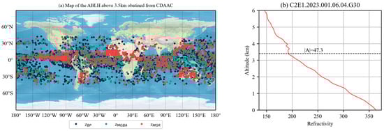
Figure 1. The COSMIC-2 RO-retrieved ABLH from CDAAC. (a) Geographic distribution of ABLH values, including $z_{MGBA}$, $z_{MGR}$, and $z_{BP}$, exceeding the threshold of 3.5 km from 1 January 2023 to 7 January 2023. (b) $z_{BP}$, violating the criterion of the BP method with |A| > 50 km⁻¹ for C2E1.2023.001.06.04.G30.

Based on the experiment conducted by Ratnam et al. (2010) [14], different dilations, ranging from 0.2 km to 0.6 km in intervals of 0.2 km, were selected. To make the dilation more representative of most GNSS-RO profiles, a single GNSS-RO profile was not chosen; instead, all the data on 29 February 2022 were selected to compare the effects of different dilations. Furthermore, it will be compared to the ABLHs calculated using other methods with GNSS-RO profiles. To avoid similarities introduced by the same refractivity profiles, bending angle profiles were used instead. Additionally, considering that the MG method was applied to the determination of AHLH with RO data earlier (than DPMF method) and has received more validation, the MGBA method will be employed.

In Figure 2, the proportions of biases > 0.2 km between $z_{MGBA}$ and $z_{WCT}$ are 54.79%, 14.56%, and 15.04%, corresponding to dilations of 0.2 km, 0.4 km, and 0.6 km, respectively. Therefore, the optimal dilation value should be set to 0.4 km.

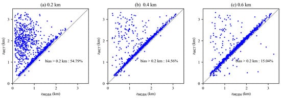
Figure 2. Scatterplots between the $z_{MGBA}$ and $z_{WCT}$ for COSMIC-2: (a) dilation: 0.2 km, (b) dilation: 0.4 km, and (c) dilation: 0.6 km.

3.2. Comparison of the RO- and RAOB-Derived ABLHs

To minimize the potential impact of landform and physiognomy on the comparison, the comparison was initiated using data in islands and coastal regions. Therefore, 61 globally distributed RAOB stations (Figure 3) on islands or along coastlines were selected to collocate with the data from GNSS-RO. Additionally, due to GNSS-RO data originating from different RO missions, it was necessary to analyze the COSMIC-2 and Spire data independently to prevent any potential systematic errors.

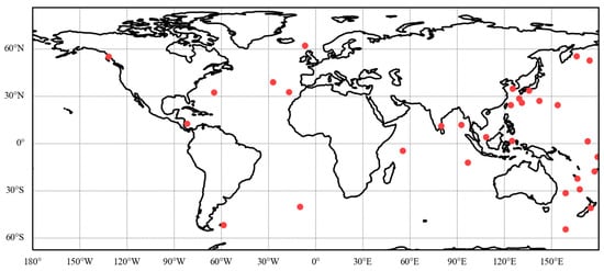
Figure 3. Location mapping: selected stations on islands or along coastlines from IGRA2 dataset.

In this study, using the ABLHs ($z_{RAOB}$) derived from RAOB atmospheric profiles as a reference, we evaluated the performances of the ABLHs ($z_{RO}$), including $z_{MGBA}$, $z_{MGR}$, $z_{BP}$, $z_{WCT}$, and $z_{DPMF}$ determined from the COSMIC-2 data using five different methods. As shown in Figure 4, the comparison results indicate a good agreement between the $z_{RAOB}$ and $z_{RO}$ over oceans. The colorbar represents a Gaussian kernel density estimation. Table 1 presents the correlation coefficients between the $z_{RAOB}$ and $z_{RO}$ derived from COSMIC-2, as well as the biases and root-mean-square error (RMSE) of the $z_{RO}$ derived from COSMIC-2 compared to the $z_{RAOB}$. Higher positive correlation coefficients for $z_{MGBA}$ (0.967), $z_{MGR}$ (0.968), $z_{BP}$ (0.966), $z_{WCT}$ (0.969), and $z_{DPMF}$ (0.967) indicate closer matching between $z_{RO}$ and $z_{RAOB}$. The differences in the correlation coefficients between $z_{RAOB}$ and $z_{RO}$ were not significant. In terms of bias and RMSE, $z_{RO}$ agreed closely with $z_{RAOB}$, and were, in descending order: $z_{MGBA}$, $z_{DPMF}$, $z_{MGR}$, $z_{WCT}$, and $z_{BP}$. $z_{MGBA}$ exhibited the smallest bias (0.023 km) with an RMSE of 0.173 km and the best agreement with $z_{RAOB}$, while $z_{BP}$ showed the most noticeable (positive) bias of 0.100 km, with an RMSE of 0.2 km.

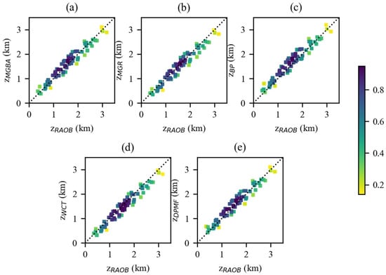
Figure 4. Scatter density plots between the $z_{RAOB}$ and $z_{RO}$ over oceans for COSMIC-2 with colorbar representing the Gaussian kernel density estimation: (a) $z_{MGBA}$, (b) $z_{MGR}$, (c) $z_{BP}$, (d) $z_{WCT}$, and (e) $z_{DPMF}$.

Table 1. The statistical analysis of the data $z_{RAOB}$ and $z_{RO}$ over oceans derived from COSMIC-2.

ABLH	Correlation Coefficient	Bias (km)	RMSE (km)
$z_{MGBA}$	0.967	0.023	0.173
$z_{MGR}$	0.968	−0.066	0.180
$z_{BP}$	0.966	0.100	0.200
$z_{WCT}$	0.969	−0.086	0.186
$z_{DPMF}$	0.967	0.034	0.175

Figure 5 shows the scatter density plots of the $z_{RAOB}$ and $z_{RO}$ over oceans determined from the Spire data, suggesting a satisfactory agreement between the $z_{RO}$ and $z_{RAOB}$, except for the $z_{WCT}$ determined using the WCT method, which had an obvious negative bias compared to the $z_{RAOB}$. Specifically, some $z_{WCT}$ values were significantly smaller than the values of corresponding $z_{RAOB}$, with biases of more than ~1.2 km. In Table 2, the correlation coefficient between the $z_{WCT}$ calculated from Spire and $z_{RAOB}$ is 0.686. Compared to the correlation between the $z_{WCT}$ derived from COSMIC-2 and $z_{RAOB}$ (0.969), the correlation weakened significantly. Moreover, the bias and RMSE were relatively large. In terms of bias and RMSE, $z_{RO}$ agreed closely with $z_{RAOB}$, and were, in descending order: $z_{MGBA}$, $z_{DPMF}$, $z_{MGR}$, $z_{BP}$, and $z_{WCT}$. The bias and RMSE for $z_{MGBA}$ remained the smallest compared to those from COMSIC-2, showing the closest agreement with $z_{RAOB}$.

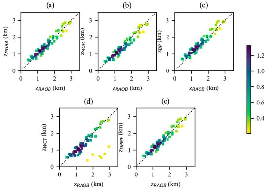
Figure 5. Scatter density plots between the $z_{RAOB}$ and $z_{RO}$ over oceans for Spire with colorbar representing the Gaussian kernel density estimation: (a) $z_{MGBA}$, (b) $z_{MGR}$, (c) $z_{BP}$, (d) $z_{WCT}$, and (e) $z_{DPMF}$.

Table 2. The statistical analysis of the data $z_{RAOB}$ and $z_{RO}$ over oceans derived from Spire.

ABLH	Correlation Coefficient	Bias (km)	RMSE (km)
$z_{MGBA}$	0.966	0.010	0.168
$z_{MGR}$	0.968	−0.088	0.190
$z_{BP}$	0.967	0.089	0.189
$z_{WCT}$	0.686	−0.243	0.562
$z_{DPMF}$	0.967	0.017	0.168

Compared to RAOB stations on islands and near coastal regions, there are more RAOB stations on land, and the ABLH over land shows a greater variability than that over the ocean. However, inland RAOB stations are more affected by landform and physiognomy. Therefore, we only considered stations with altitudes below 0.5 km, located deep inland at least 300 km away from the coast, to avoid the influence of coastal and oceanic areas. The distribution of inland RAOB stations is shown in Figure 6.

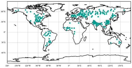
Figure 6. Location mapping: selected stations over land from IGRA2 dataset.

Figure 7 displays the scatter density plots of the $z_{RAOB}$ and $z_{RO}$ calculated from the COSMIC-2 data for inland regions. Table 3 shows the statistical analysis results of the $z_{RAOB}$ and $z_{RO}$ inland from the COSMIC-2 data. Combining the statistical results from Table 3, the main findings and the results from the $z_{RO}$ over oceans for Spire were similar. The number of RO profiles over oceans was relatively limited, which may explain why smaller $z_{WCT}$ values were not found in the COSMIC-2 oceanic data. This suggests that the cause of the significantly lower $z_{WCT}$ compared to $z_{RAOB}$ was likely inherent to the WCT method itself, rather than the Spire RO data.

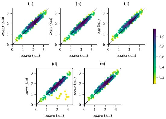
Figure 7. Scatter density plots between the $z_{RAOB}$ and $z_{RO}$ inland for COSMIC-2 with colorbar representing the Gaussian kernel density estimation: (a) $z_{MGBA}$, (b) $z_{MGR}$, (c) $z_{BP}$, (d) $z_{WCT}$, and (e) $z_{DPMF}$.

Table 3. The statistical analysis of the data $z_{RAOB}$ and $z_{RO}$ inland derived from COSMIC-2.

ABLH	Correlation Coefficient	Bias (km)	RMSE (km)
$z_{MGBA}$	0.970	0.010	0.155
$z_{MGR}$	0.970	−0.199	0.185
$z_{BP}$	0.969	0.087	0.179
$z_{WCT}$	0.814	−0.204	0.437
$z_{DPMF}$	0.970	0.023	0.157

In Figure 8, the scatter density plots of the $z_{RAOB}$ and $z_{RO}$ inland calculated from the Spire data are shown. Table 4 presents the statistical analysis results of the $z_{RAOB}$ and $z_{RO}$ from the Spire data for inland regions. In Figure 8, the ABLHs calculated by Spire in the range from 1 to 1.5 km are denser compared to COSMIC-2. There is a greater quantity of data in the range from 1 to 1.5 km, in contrast to the inland ABLHs obtained from COSMIC-2. This was mainly because COSMIC-2 is concentrated in mid-latitude regions, whereas Spire offers global coverage. The ABLH in mid-latitude regions was higher compared to that in high-latitude regions [24].

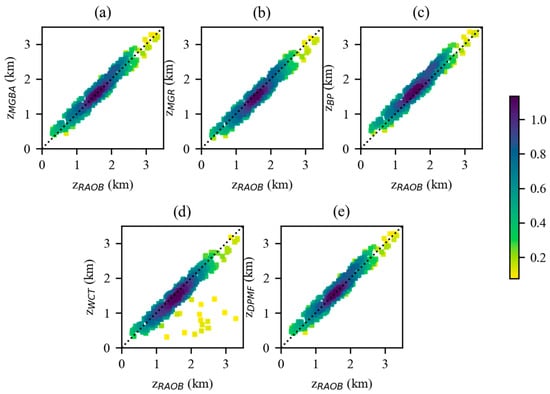
Figure 8. Scatter density plots between the $z_{RAOB}$ and $z_{RO}$ inland for Spire with colorbar representing the Gaussian kernel density estimation: (a) $z_{MGBA}$, (b) $z_{MGR}$, (c) $z_{BP}$, (d) $z_{WCT}$, and (e) $z_{DPMF}$.

Table 4. The statistical analysis of the data $z_{RAOB}$ and $z_{RO}$ inland derived from Spire.

ABLH	Correlation Coefficient	Bias (km)	RMSE (km)
$z_{MGBA}$	0.965	0.024	0.170
$z_{MGR}$	0.964	−0.073	0.185
$z_{BP}$	0.965	0.108	0.201
$z_{WCT}$	0.828	−0.164	0.406
$z_{DPMF}$	0.965	0.036	0.174

Based on the statistical data presented in Table 1, Table 2, Table 3 and Table 4, it can be observed that there were no significant differences in the biases and RMSE of the $z_{RO}$ from Spire and COSMIC-2 compared to the $z_{RAOB}$, except in the case of the WCT method. As multiple reports and studies have already compared and evaluated data from both COSMIC-2 and Spire, and considering the high similarity in the bending angle and refractivity accuracy [25,26], we will not discuss these aspects separately in the following content.

Figure 9 illustrates the biases and RMSE of the $z_{RO}$ over oceans in the Northern Hemisphere using the five different methods across four seasons (MAM: from March to May, JJA: from June to August, SON: from September to November, and DJF: from December to February). Specially, $z_{WCT}^{*}$ represents the $z_{WCT}$ without a bias of more than 1.2 km with $z_{RAOB}$. In all four seasons, $z_{WCT}$ consistently had the largest bias and RMSE among the five methods. Notably, the biases of $z_{WCT}$ and $z_{WCT}^{*}$ exhibited seasonal variability, with the highest biases being observed during JJA and the lowest during DJF. Conversely, the RMSE values for the $z_{MGBA}$, $z_{MGR}$, $z_{BP}$, and $z_{DPMF}$ did not exhibit pronounced seasonal variations. The biases of $z_{WCT}^{*}$ were smaller than those of $z_{WCT}$, which was due to the removal of data with biases exceeding 1.2 km. The RMSE of $z_{WCT}$ was then relatively close to that of other $z_{RO}$. However, the biases and RMSE of $z_{WCT}^{*}$ still showed some seasonal characteristics, possibly because larger biases were not completely removed, and the lower number of collocated RO profiles over oceans made it difficult to effectively reduce errors through averaging. It is possible that this was caused by the lower quality of the GNSS-RO refractivity profiles near the Earth’s surface. Near the surface, super-refraction and signal tracking errors are more likely to occur, leading to negative biases in refractivity [27,28,29]. Environments with high humidity are more prone to inducing super-refraction [30]. As a result, the bias and RMSE of $z_{WCT}$ are more likely to exhibit seasonal variations. Further analysis will be conducted in Section 3.4.

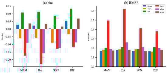
Figure 9. Biases (a) and RMSE (b) of $z_{RO}$ over oceans in the Northern Hemisphere using five methods. The data are grouped into four different seasons (MAM: from March to May, JJA: from June to August, SON: from September to November, and DJF: from December to February). $z_{WCT}^{*}$ represents the $z_{WCT}$ without a bias of more than 1.2 km with $z_{RAOB}$.

In Figure 10, the deviation and RMSE between $z_{RO}$ and $z_{RAOB}$ within the Northern Hemisphere’s inland regions are presented. It can be observed that the $z_{WCT}^{*}$ in inland areas did not exhibit significant seasonal variations, due to a larger number of profiles, which helped to reduce errors through averaging. From Table 1, Table 2, Table 3 and Table 4 and Figure 9 and Figure 10, it is evident that $z_{MGBA}$ performed the best and was closest to the RAOB measurements.

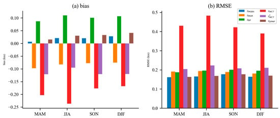
Figure 10. Biases (a) and RMSE (b) of $z_{RO}$ inland in the Northern Hemisphere using five methods. The data are grouped into four different seasons (MAM: from March to May, JJA: from June to August, SON: from September to November, and DJF: from December to February). $z_{WCT}^{*}$ represents the $z_{WCT}$ without a bias of more than 1.2 km with $z_{RAOB}$.

3.3. Comparison of the RO-Derived ABLHs

The comparisons between the ABLHs derived from the RO data and the RAOB in Section 3.1 are restricted only to the vicinity of RAOB stations. To further compare the ALBHs derived from RO data on a large spatial scale, we conducted a comprehensive investigation of MBLHs globally. Based on the above analysis, $z_{MGBA}$ exhibited the smallest error. Therefore, we used $z_{MGBA}$ as a reference value to analyze other $z_{RO}$.

Figure 11 shows the annual-averaged differences of $z_{MGR}$, $z_{BP}$, $z_{WCT}$, and $z_{DPMF}$ w.r.t. $z_{MGBA}$ over oceans for the period from 1 March 2022 to 28 February 2023 in a given latitude–longitude bin with a resolution of 1° × 1°. In ascending order w.r.t. the differences from $z_{MGBA}$, they were $z_{WCT}$, $z_{MGR}$, $z_{DPMF}$, and $z_{BP}$. Specifically, the differences for $z_{WCT}$ and $z_{MGR}$ were negative, while those for $z_{DPMF}$ and $z_{BP}$ were positive. The $z_{WCT}$ values were relatively lower than the other $z_{RO}$ values. This was because $z_{WCT}$ exhibited a significant negative bias, as presented in Section 3.2.

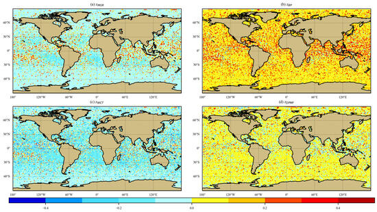
Figure 11. The annual-averaged differences of (a) $z_{MGR}$, (b) $z_{BP}$, (c) $z_{WCT}$, and (d) $z_{DPMF}$ w.r.t. $z_{MGBA}$ over oceans from 1 March 2022 to 28 February 2023 in a given latitude–longitude bin (1° × 1°).

The boxplot in Figure 12 graphically shows the distribution of the MBLHs determined by the five methods from 1 March 2022 to 28 February 2023. The box extends from the first quartile (Q1) to the third quartile (Q3), and the yellow line indicates the median value. More detailed information on the median, Q1, and Q3 values for the MBLHs obtained using each method can be found in Table 5. Among the five methods, the distributions of $z_{MGBA}$ and $z_{DPMF}$ showed a better agreement with each other than with the others, with a median value of about 1.6 km. Compared to $z_{MGBA}$ and $z_{DPMF}$, the median value of $z_{BP}$ (1.820) was relatively high, while the median value of $z_{MGR}$ (1.598) wazs relatively low. The values of $z_{WCT}$, on the other hand, were significantly lower than those of the other methods, which is consistent with the results presented in Section 3.2.

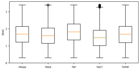
Figure 12. The boxplot of the MBLHs using the five methods from 1 March 2022 to 28 February 2023.

Table 5. The median, first quartile (Q1), and third quartile (Q3) of $z_{RO}$.

ABLH	Median (km)	Q1 (km)	Q3 (km)
$z_{MGBA}$	1.689	1.220	2.138
$z_{MGR}$	1.598	1.451	2.045
$z_{BP}$	1.820	1.345	2.283
$z_{WCT}$	1.475	1.010	1.974
$z_{DPMF}$	1.686	1.867	2.145

3.4. Analysis on the Biases of the RO-Derived ABLHs

The experimental analysis mentioned above involved the outlier screening of $z_{RO}$ using the five methods. $z_{WCT}$ was consistently lower than the ABLHs obtained using other methods. This discrepancy may be attributed to the sensitivity of the WCT method to refractivity mutations near the Earth’s surface. In this case, outlier screening was removed to facilitate the comparison of the differences among the five methods, especially the WCT method.

Compared to Figure 12 and Table 5, as shown in Figure 13 and Table 6, the median values of the MBLH calculated using the five methods decreased. This was due to the outlier screening process, which removed data with larger differences. MBLH values near the Earth’s surface are more numerous and contain more errors, making them more likely to be removed. Without outlier screening, the number of smaller values for $z_{WCT}$ would increase noticeably, followed by $z_{DPMF}$. In contrast, the boxplots of the other three methods show relatively small variations after the outlier screening (as seen in Figure 12). The DPMF and WCT methods attempt to utilize data near the lower troposphere more extensively than the other three methods. However, the RO profiles near the lower troposphere are associated with larger errors and significant variations, resulting in the unreliability of the $z_{WCT}$ and $z_{DPMF}$.

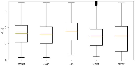
Figure 13. The boxplot of the MBLHs without outlier screening using the five methods from 1 March 2022 to 28 February 2023.

Table 6. The median, first quartile (Q1), and third quartile (Q3) of $z_{RO}$ without outlier screening.

ABLH	Median (km)	Q1 (km)	Q3 (km)
$z_{MGBA}$	1.626	1.087	2.118
$z_{MGR}$	1.536	1.017	2.027
$z_{BP}$	1.758	1.222	2.265
$z_{WCT}$	1.407	0.892	1.882
$z_{DPMF}$	1.469	0.530	2.056

As shown in Figure 14, a GNSS-RO event profile of bending angle (red line) and refractivity (blue line) was selected to further analyze the biases of the RO-derived ABLHs. The WCT and DPMF methods detected strong variations in the profiles near the Earth’s surface and considered them as ABLHs. Through comparison to $z_{RAOB}$, it became evident that these pronounced fluctuations were more likely caused by errors. Using other three $z_{RO}$ as auxiliary information, the heights of the minimum points closest to the values of other three $z_{RO}$ were considered as the ABLHs obtained using WCT and DPMF (corresponding to $z_{WCT}^{\prime }$ and $z_{DPMF}^{\prime }$).

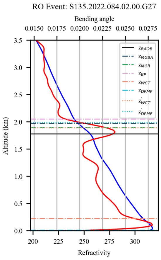
Figure 14. The GNSS-RO event profile of bending angle (red line) and refractivity (blue line) with five $z_{RO}$. $z_{WCT}^{\prime }$ and $z_{DPMF}^{\prime }$ represented using $z_{RO}$ with the other three methods as auxiliary information to determine the correct ABLH by selecting the minimum point heights from the three methods closest to them.

Basing their values on the other three $z_{RO}$, the occurrence of significantly lower values in the case of the $z_{WCT}$ and $z_{DPMF}$ was considered as an outlier. We conducted a statistical analysis on the occurrence of lower values for $z_{WCT}$ and $z_{DPMF}$ from 1 March 2022 to 28 February 2023, and found that the probabilities were 10.50% and 4.24%, respectively.

4. Discussion

Overall, our study focused on the comparison and evaluation of ABLH estimation methods using data from various sources, including GNSS-RO and RAOB. We analyzed five different methods: MGBA, MGR, BP, WCT, and DPMF.

First, we analyzed the raw ABLHs provided by the CDAAC and identified the significant discrepancies and inconsistencies in the $z_{MGBA}$, $z_{MGR}$, and $z_{BP}$ values that did not align with the established criteria. As a result, we opted to derive $z_{MGBA}$, $z_{MGR}$, and $z_{BP}$ using our own calculations and applied outlier screening based on predefined criteria. This ensured the reliability and accuracy of the ABLH data used in our comparative study. Furthermore, an analysis of the optimal dilation value for WCT was conducted. Based on extensive data statistics, the optimal value was determined to be 0.4 km.

In terms of correlation, $z_{MGBA}$, $z_{MGR}$, $z_{BP}$, and $z_{DPMF}$ demonstrated strong positive correlations with $z_{RAOB}$. When considering biases and RMSE, $z_{MGBA}$ exhibited minimal errors, showing relatively small biases and RMSE values that closely aligned with the reference $z_{RAOB}$. In contrast, the WCT method stood out with a little weaker correlation, noticeable bias, and higher RMSE. $z_{WCT}$ occasionally exhibited some low values, causing a decrease in correlation, as well as increases in bias and RMSE.

A seasonal analysis revealed that the bias in the ABLH estimations for $z_{MGBA}$, $z_{MGR}$, $z_{BP}$, and $z_{DPMF}$ exhibited no obvious seasonal variability. Notably, the biases of $z_{WCT}$ exhibited seasonal variability, with the highest biases being observed during JJA and the lowest during DJF. It is possible that this was caused by the lower quality of the GNSS-RO refractivity profiles near the Earth’s surface. Near the surface, super-refraction and signal tracking errors are more likely to occur, leading to negative biases in refractivity [27,28,29]. Environments with high humidity are more prone to inducing super-refraction [30]. As a result, the bias and RMSE of $z_{WCT}$ were more likely to exhibit seasonal variations.

Furthermore, we investigated the global distribution of the MBLHs obtained using the five methods. While $z_{MGBA}$,$z_{DPMF}$ and $z_{MGR}$ exhibited minimal differences, the $z_{WCT}$ values were relatively lower than the other $z_{RO}$ values, while the $z_{BP}$ values were relatively higher than the other $z_{RO}$ values.

Eventually, we removed the outlier screening to facilitate a comparison of the differences among the five methods. The WCT and DPMF methods could detect strong variations in the profiles near the Earth’s surface and considered them as ABLH. Through a comparison to $z_{RAOB}$, it became evident that these pronounced fluctuations were more likely caused by errors.

In summary, these findings have important implications for selecting appropriate methods for ABLH estimation. The MGBA method emerged as a reliable and stable option, while the WCT and DPMF methods should be used with caution due to the lower quality of the GNSS-RO refractivity profiles near the Earth’s surface. Furthermore, the DPMF method has its shortcomings, including lengthy computations and the possibility of failed iterative calculations. The MGR and BP methods also showed promising performances.

5. Conclusions

In this work, our study compared five ABLH estimation methods using GNSS-RO and RAOB data. Based on the above assessment and analysis, the following conclusions can be drawn:

• $z_{MGBA}$ exhibited minimal errors, showing relatively small biases and RMSE values that closely aligned with the reference $z_{RAOB}$.
• $z_{WCT}$ occasionally exhibited some low values, causing a decrease in correlation, as well as increases in bias and RMSE.
• A seasonal analysis revealed that the bias in the ABLH estimations for $z_{MGBA}$, $z_{MGR}$, $z_{BP}$, and $z_{DPMF}$ exhibited no obvious seasonal variability. Notably, the biases of $z_{WCT}$ exhibited seasonal variability, with the highest biases being observed during JJA and the lowest during DJF.
• The WCT and DPMF methods could detect strong variations in the profiles near the Earth’s surface and considered them as ABLH. However, these variations were caused by errors. They should be used with caution due to the lower quality of the GNSS-RO bending angle or refractivity profiles near the Earth’s surface.

This research comprehensively compared ABLH estimation methods, with MGBA standing out for its exceptional performance. It offers highly accurate ABLH estimates that closely agree with RAOB-derived ABLHs, providing robust support for precise atmospheric boundary layer height estimation.

References

- Garratt, J.R. The Atmospheric Boundary Layer; Cambridge atmospheric and space science series; Cambridge University Press: Cambridge, UK, 1992. [Google Scholar]
- Seibert, P.; Beyrich, F.; Gryning, S.-E.; Joffre, S.; Rasmussen, A.; Tercier, P. Review and intercomparison of operational methods for the determination of the mixing height. Atmos. Environ. 2000, 34, 1001–1027. [Google Scholar] [CrossRef]
- Kotthaus, S.; Bravo-Aranda, J.A.; Collaud Coen, M.; Guerrero-Rascado, J.L.; Costa, M.J.; Cimini, D.; O’Connor, E.J.; Hervo, M.; Alados-Arboledas, L.; Jiménez-Portaz, M.; et al. Atmospheric boundary layer height from ground-based remote sensing: A review of capabilities and limitations. Atmos. Meas. Tech. 2023, 16, 433–479. [Google Scholar] [CrossRef]
- Schreiner, W.S.; Weiss, J.P.; Anthes, R.A.; Braun, J.; Chu, V.; Fong, J.; Hunt, D.; Kuo, Y.-H.; Meehan, T.; Serafino, W.; et al. COSMIC-2 Radio Occultation Constellation: First Results. Geophys. Res. Lett. 2020, 47, e2019GL086841. [Google Scholar] [CrossRef]
- Ho, S.-P.; Zhou, X.; Shao, X.; Zhang, B.; Adhikari, L.; Kireev, S.; He, Y.; Yoe, J.G.; Xia-Serafino, W.; Lynch, E. Initial Assessment of the COSMIC-2/FORMOSAT-7 Neutral Atmosphere Data Quality in NESDIS/STAR Using In Situ and Satellite Data. Remote Sens. 2020, 12, 4099. [Google Scholar] [CrossRef]
- Von Engeln, A.; Teixeira, J.; Wickert, J.; Buehler, S.A. Using CHAMP radio occultation data to determine the top altitude of the Planetary Boundary Layer. Geophys. Res. Lett. 2005, 32, L06815–L06818. [Google Scholar] [CrossRef]
- Sokolovskiy, S.; Kuo, Y.-H.; Rocken, C.; Schreiner, W.S.; Hunt, D.; Anthes, R.A. Monitoring the atmospheric boundary layer by GPS radio occultation signals recorded in the open-loop mode. Geophys. Res. Lett. 2006, 33, L12813–L12816. [Google Scholar] [CrossRef]
- Guo, P.; Kuo, Y.-H.; Sokolovskiy, S.V.; Lenschow, D.H. Estimating Atmospheric Boundary Layer Depth Using COSMIC Radio Occultation Data. J. Atmos. Sci. 2011, 68, 1703–1713. [Google Scholar] [CrossRef]
- Chan, K.M.; Wood, R. The seasonal cycle of planetary boundary layer depth determined using COSMIC radio occultation data. J. Geophys. Res. Atmos. 2013, 118, 12, 422-12, 434. [Google Scholar] [CrossRef]
- Basha, G.; Ratnam, M.V. Identification of atmospheric boundary layer height over a tropical station using high-resolution radiosonde refractivity profiles: Comparison with GPS radio occultation measurements. J. Geophys. Res. Atmos. 2009, 114, D16101–D16111. [Google Scholar] [CrossRef]
- Ao, C.O.; Waliser, D.E.; Chan, S.K.; Li, J.-L.; Tian, B.; Xie, F.; Mannucci, A.J. Planetary boundary layer heights from GPS radio occultation refractivity and humidity profiles. J. Geophys. Res. Atmos. 2012, 117, D16117–D16134. [Google Scholar] [CrossRef]
- Sokolovskiy, S.V.; Rocken, C.; Lenschow, D.H.; Kuo, Y.-H.; Anthes, R.A.; Schreiner, W.S.; Hunt, D.C. Observing the moist troposphere with radio occultation signals from COSMIC. Geophys. Res. Lett. 2007, 34, L18802–L18807. [Google Scholar] [CrossRef]
- Xie, F.; Wu, D.L.; Ao, C.O.; Mannucci, A.J.; Kursinski, E.R. Advances and limitations of atmospheric boundary layer observations with GPS occultation over southeast Pacific Ocean. Atmos. Chem. Phys. 2012, 12, 903–918. [Google Scholar] [CrossRef]
- Ratnam, M.V.; Basha, S.G. A robust method to determine global distribution of atmospheric boundary layer top from COSMIC GPS RO measurements. Atmos. Sci. Lett. 2010, 11, 216–222. [Google Scholar] [CrossRef]
- Xu, X.; Li, Y.; Luo, J. Marine Boundary Layer Heights in the Tropical and Subtropical Oceans Derived from COSMIC-2 Radio Occultation Data. Adv. Atmos. Sci. 2023, 40, 1058–1072. [Google Scholar] [CrossRef]
- Yan, S.; Xiang, J.; Du, H. Determining Atmospheric Boundary Layer Height with the Numerical Differentiation Method Using Bending Angle Data from COSMIC. Adv. Atmos. Sci. 2019, 36, 303–312. [Google Scholar] [CrossRef]
- Zhou, J.; Xiang, J.; Huang, S. Marine Boundary Layer Height Obtained by New Numerical Regularization Method Based on GPS Radio Occultation Data. Sensors 2020, 20, 4762. [Google Scholar] [CrossRef]
- Ho, S.-p.; Peng, L.; Anthes, R.A.; Kuo, Y.-H.; Lin, H.-C. Marine Boundary Layer Heights and Their Longitudinal, Diurnal, and Interseasonal Variability in the Southeastern Pacific Using COSMIC, CALIOP, and Radiosonde Data. J. Clim. 2015, 28, 2856–2872. [Google Scholar] [CrossRef]
- Chen, S.-Y.; Liu, C.-Y.; Huang, C.-Y.; Hsu, S.-C.; Li, H.-W.; Lin, P.-H.; Cheng, J.-P.; Huang, C.-Y. An Analysis Study of FORMOSAT-7/COSMIC-2 Radio Occultation Data in the Troposphere. Remote Sens. 2021, 13, 717. [Google Scholar] [CrossRef]
- Masters, D.; Nguyen, V.; Irisov, V.; Nogues-Correig, O.; Tan, L.; Yuasa, T.; Ringer, J.; Rocken, C.; Gorbunov, M. Commercial RO Becomes Reality: Rapid Growth, External Validation, and Operational Assimilation of Spire RO. In Proceedings of the 8th International Radio Occultation Working Group Meeting, Virtual Meeting, 7–13 April 2021. [Google Scholar]
- Gamage, N.; Hagelberg, C. Detection and Analysis of Microfronts and Associated Coherent Events Using Localized Transforms. J. Atmos. Sci. 1993, 50, 750–756. [Google Scholar] [CrossRef]
- Brooks, I.M. Finding Boundary Layer Top: Application of a Wavelet Covariance Transform to Lidar Backscatter Profiles. J. Atmos. Ocean. Technol. 2003, 20, 1092–1105. [Google Scholar] [CrossRef]
- Schreiner, B.; Kuo, B.; Rocken, C.; Sokolovskiy, S.; Hunt, D.; Ho, B.; Yue, X.; Wee, T.; Hudnut, K.; Sleziak-Sallee, M. COSMIC Data Analysis and Archive Center (CDAAC) Current Status and Future Plans; International Radio Occultation Working Group-4: Boulder, CO, USA, 2014. [Google Scholar]
- Basha, G.; Kishore, P.; Ratnam, M.V.; Ravindra Babu, S.; Velicogna, I.; Jiang, J.H.; Ao, C.O. Global climatology of planetary boundary layer top obtained from multi-satellite GPS RO observations. Clim. Dyn. 2019, 52, 2385–2398. [Google Scholar] [CrossRef]
- Irisov, V.; Nguyen, V.; Masters, D.; Sikarin, R.; Bloom, A.; Gorbunov, M.; Rocken, C. Comparison of Spire RO profiles Processed by UCAR and Spire. In Proceedings of the 8th International Radio Occultation Working Group Meeting, Virtual Meeting, 7–13 April 2021. [Google Scholar]
- Jing, X.; Ho, S.-P.; Shao, X.; Liu, T.-C.; Chen, Y.; Zhou, X. Spire RO Thermal Profiles for Climate Studies: Initial Comparisons of the Measurements from Spire, NOAA-20 ATMS, Radiosonde, and COSMIC-2. Remote Sens. 2023, 15, 3710. [Google Scholar] [CrossRef]
- Sokolovskiy, S. Effect of superrefraction on inversions of radio occultation signals in the lower troposphere. Radio Sci. 2003, 38, 1058–1071. [Google Scholar] [CrossRef]
- Xie, F.; Syndergaard, S.; Kursinski, E.R.; Herman, B.M. An Approach for Retrieving Marine Boundary Layer Refractivity from GPS Occultation Data in the Presence of Superrefraction. J. Atmos. Ocean. Technol. 2006, 23, 1629–1644. [Google Scholar] [CrossRef]
- Yu, X.; Xie, F.; Ao, C.O. Evaluating the lower-tropospheric COSMIC GPS radio occultation sounding quality over the Arctic. Atmos. Meas. Tech. 2018, 11, 2051–2066. [Google Scholar] [CrossRef]
- Johnston, B.R.; Randel, W.J.; Sjoberg, J.P. Evaluation of Tropospheric Moisture Characteristics Among COSMIC-2, ERA5 and MERRA-2 in the Tropics and Subtropics. Remote Sens. 2021, 13, 880. [Google Scholar] [CrossRef]
Disclaimer/Publisher’s Note: The statements, opinions and data contained in all publications are solely those of the individual author(s) and contributor(s) and not of MDPI and/or the editor(s). MDPI and/or the editor(s) disclaim responsibility for any injury to people or property resulting from any ideas, methods, instructions or products referred to in the content. |
© 2023 by the authors. Licensee MDPI, Basel, Switzerland. This article is an open access article distributed under the terms and conditions of the Creative Commons Attribution (CC BY) license (https://creativecommons.org/licenses/by/4.0/).