Abstract
Extreme rainfall is the main contributing factor to landslides. Therefore, it is of great significance to monitor and forecast short-term rainfall in landslide-prone areas. However, the spatial scale of landslide-prone areas is small, and traditional numerical forecast models have difficulty in accurately forecasting rainfall on this scale. To solve the above problem, this study proposes a short-term rainfall forecasting method for landslide-prone areas by combining the back-propagation neural network (BP-NN) algorithm and global navigation satellite system (GNSS) observations to achieve accurate short-term rainfall forecasting in landslide-prone areas. Firstly, a high-precision atmospheric weighted-average temperature (Tm) model is established using radiosonde data to obtain high-precision precipitable water vapor (PWV) estimates. Secondly, the BP-NN algorithm is introduced, and the GNSS-derived PWV, temperature and pressure from a meteorological station, and rainfall for the previous and next hour are used as input parameters to establish a BP-NN-based rainfall forecast model. As an illustrative case, experiments are conducted in a landslide-prone area in Yunnan Province using data from 15 GNSS stations and the corresponding meteorological station. Statistical results show that the established regional Tm model has high accuracy, with an average root mean square (RMS) and bias of 3 K and 0.15 K, respectively. In addition, the short-term rainfall forecast model based on the BP algorithm achieves a true detection rate of up to 93.70% and a false forecast rate of as low as 38.30%, which is significant for short-term rainfall forecasting in landslide-prone areas.
1. Introduction
Landslides are a serious threat to human life, property, and the living environment. According to statistics from the Centre for Research on the Epidemiology of Disasters (CRED) released in 2014, in the 20th century, approximately 13,000 people worldwide died every year as a result of landslides and flooding events, resulting in economic losses exceeding 500 billion US dollars [1]. Rainfall is the main contributing factor to landslides, and the months with a high frequency of landslides are the same as those with frequent heavy rainfall events [2,3]. Therefore, an accurate warning of short-term heavy rainfall with a lead time of several hours would help reduce the impact of landslides on human activities.
In the field of rainfall-based landslide warning research, Moya-Álvarez et al. [4] completed a precipitation threshold equation test experiment by collecting precipitation data from 96 landslide-prone areas in South Africa’s Campania region. They also proposed a rainfall-based landslide-prone area warning model based on the precipitation threshold. Ma et al. [5] developed a comprehensive landslide monitoring and warning system for the Norwegian Meteorological Institute based on five key components: automatic hydrological and meteorological stations, landslide and flood historical databases, hydrometeorological forecast models, landslide forecast models, and threshold or return period. Pal et al. [6] used the Internet of Things technology to continuously monitor slopes around the Himalayas and studied the relationship between slope angle, water content, and precipitation. They also proposed a precipitation threshold suitable for the region and established a landslide monitoring and warning system based on precipitation as the primary warning indicator. However, although the preceding studies have constructed rainfall threshold conditions applicable for providing warnings of possible landslides, they have not issued warnings for short-term heavy rainfall events in landslide-prone areas. Therefore, there are still limitations in forecasting landslide events caused by short-term heavy rainfall events.
In recent years, the global navigation satellite system (GNSS) has been extensively employed for remote sensing of atmospheric water vapor and monitoring extreme weather conditions [7]. Atmospheric water vapor can be reflected by precipitable water vapor (PWV), a measure of the total water vapor in the air column of a unit cross-section from the ground to the top of the atmosphere [8]. Compared with traditional water vapor retrieval techniques, GNSS-derived PWV has advantages such as high accuracy, high temporal and spatial resolution, low cost, and all-weather availability. GNSS-derived PWV, as a key parameter of GNSS meteorology, has also been used to forecast rainfall events in recent years. Benevides et al. [9] used the least squares principle to analyze the long-term trend in PWV and found that most rainfall events occurred during the short period after a short-term accumulation in PWV. Based on the above findings, a short-term rainfall warning model was proposed suitable for Portugal’s Lisbon region, using the maximum growth rate in PWV as the forecasting factor. The true detection rate (TDR) of the proposed rainfall forecast model was approximately 75%, while the false forecast rate (FFR) was 60–70%. Zhao et al. [10] proposed a rainfall forecasting method combining two tropospheric parameters, zenith tropospheric delay (ZTD) and PWV, to improve the accuracy of rainfall warnings, which addressed the low accuracy and high FFR of existing methods. Their experimental results showed that with their approach, the TDR could reach over 95%, and the FFR was only about 30%. Li et al. [11] developed a novel cumulative-anomaly-based model (NCAM) by incorporating 14 predictive factors including ZTD and PWV. Their results showed that the NCAM model can accurately forecast 99.1% of heavy rainfall events with a lead time of 2.87 h and with an FFR of only 22.4%.
The back-propagation neural network (BP-NN) is a type of multilayer feedforward artificial neural network with memory association, which has the advantages of the ability to solve complex internal mechanism problems, independent learning and adaptation, and parallel processing. In addition, neural networks can extract input–output relationships without clear physical conditions and use error gradient descent algorithms to minimize mean squared errors between outputs. Therefore, neural networks are suitable for meteorological forecasting applications [12,13]. Hashim et al. [14] found that BP-NN is suitable for rainfall forecasts using various meteorological parameters, such as temperature, pressure, and humidity. Srivastava et al. [15] used artificial neural network algorithms to forecast daily precipitation in northern India and achieved good forecast results (Srivastava et al. 2017). Guan et al. [16] applied the BP-NN algorithm to the generation of high-precision rainfall forecasts at 26 stations in the Chaohe region from 1958 to 2012 and achieved good rainfall forecast results. Benevides et al. [17] used GNSS-derived PWV data and various meteorological parameters to establish a nonlinear autoregressive exogenous neural network model (NARX) for detecting heavy rainfall events. Li et al. [18] established a BP-NN rainfall forecast model by taking seven meteorological variables as input data for detecting heavy precipitation. Although previous research on rainfall warnings using the BP-NN algorithm and GNSS data has achieved good results in urban areas, the applicability of existing studies to landslide-prone areas has not previously been analyzed. To further validate the potential flexibility of this method for rainfall forecasting, this study proposes a novel rainfall forecast method by combining the BP-NN algorithm and GNSS observations for landslide-prone areas. The proposed method can forecast rainfall events in the next 2–6 h, and 15 GNSS stations and corresponding meteorological data from a landslide-prone area in Yunnan Province are selected to validate the performance of the proposed method. Experimental results show that the proposed method has a good potential for rainfall forecasting in landslide-prone areas.
2. Study Area and Data Description
2.1. Study Area
A landslide-prone slope located in a specific autonomous county in Yunnan Province is selected as the study area. The county is characterized by high mountain canyons, continuous mountain ranges, rugged terrain, and winding rivers. The terrain gradually ascends from south to north, with altitudes of 1620–4880 m. The area belongs to a subtropical monsoon climate with even rainfall distribution, with an annual average temperature is 16.9 °C, and with an annual average rainfall of up to 1096.5 mm. The overall geomorphic form of the selected slope is fan-shaped. A total of 15 GNSS stations have been installed in the landslide-prone area since May 2020. The geographical distribution of the GNSS stations used in the experiment is shown in Figure 1.
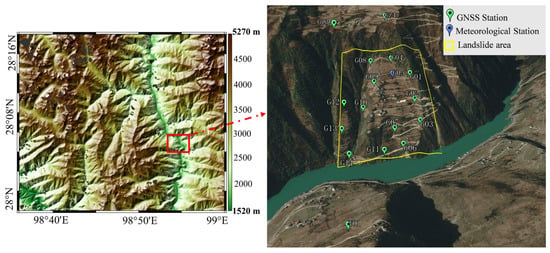
Figure 1.
Geographical distributions of the GNSS and meteorological stations in the selected landslide-prone area in Yunnan Province.
2.2. Data Description
- (1)
- GNSS data
Four GNSS stations (G01, G02, GZ3, and T01) located in the selected landslide-prone area are used as examples for the experiment, which covered the whole of 2021, with a data sampling rate of 15 s. The geodetic heights of the four selected GNSS stations are 2194.69 m, 2078.24 m, 2434.86 m, and 2172.61 m, respectively. The observation data are processed using the precise point positioning (PPP) technique. The PPP technique is a data processing method for pseudo-range and carrier phase observations received by one GNSS receiver that makes use of accurate error correction models and precise satellite ephemeris and clock offset information. The PPP software used in this paper used extended Kalman filtering for parameter estimation, while receiver coordinates, zenith tropospheric delay (ZTD), and receiver clock error were estimated as unknown parameters. Table 1 gives the specific processing strategy for the PPP technique.

Table 1.
Specific data processing strategies for the PPP technique.
- (2)
- Radiosonde data
The Integrated Global Radiosonde Archive Version 1 (IGRA Ver. 1) was created by the US National Climatic Data Center (NCDC) in the 1960s. IGRA Ver. 1 uses sensors installed on radiosonde balloons to collect meteorological data, such as temperature, pressure, humidity, and wind speed, at various heights from the ground up to 30 km. Thereafter, these observations are transmitted to ground stations [20]. IGRA provides important meteorological parameters, such as temperature, pressure, and water vapor, at altitudes of up to about 30 km above ground level for over 1500 stations worldwide [21]. In August 2016, NCDC released the second generation IGRA (IGRA2), which is superior to IGRA Ver. 1 in terms of the number of stations, observation duration, and data sources. In this study, 12 radiosonde stations from IGRA2 located around the landslide-prone area are selected to construct a regional atmospheric weighted-average temperature model (Tm) for the calculation of high-precision PWV using GNSS observations.
- (3)
- ECMWF data
The ERA5 data set, released by the European Centre for Medium-Range Weather Forecasts (ECMWF) on 14 June 2018, is a fifth-generation re-analysis product of the ECMWF. It contains hourly global atmospheric, land surface, and oceanic parameters from 1950 to the present. This data set provides atmospheric parameters at 37 pressure levels, with a spatial resolution of 0.25° × 0.25°. Compared with the equivalent fourth-generation re-analysis data (ERA-interim), ERA5 uses the latest Integrated Forecast System (IFS) Cy41r2 and has a higher horizontal resolution of 31 km (compared with 80 km) and a higher temporal resolution of 1 h (compared with 6 h). Therefore, ERA5 data (i.e., pressure, temperature, and PWV) in the landslide-prone area from 2021 were employed for experimental validation.
3. Methodology
3.1. Retrieval of GNSS-Derived PWV
ZTD includes two components, namely, zenith wet delay (ZWD) and zenith hydrostatic delay (ZHD), which account for approximately 10% and 90% of ZTD, respectively. The atmospheric water vapor content can be calculated from ZWD [10]. For the retrieval of GNSS-derived PWV, the GNSS observation is first processed using PPP or relative positioning techniques to estimate high-precision ZTD values [22,23]. ZHD can be calculated using the Saastamoinen model, which combines station position information, geodetic height values, and pressure observations [24].
where is the surface pressure (hPa), is the elevation of the GNSS station, and is the geographical latitude of the GNSS station. Therefore, ZWD can be further calculated as follows: ZWD = ZTD − ZHD. Lastly, ZWD is converted into PWV in the zenith direction through a conversion factor [25], which is expressed as follows:
where the conversion factor can be calculated using the . The calculation expression is as follows:
where is the density of water (1.0 × 10³ kg/m3), is the gas constant of atmospheric water vapor (461.495), and are the refractive constants of the atmosphere, and is calculated based on empirical formulas. In this study, a regional model is established.
3.2. Establishment of High-Precision Regional Tm Model
Yao et al. [26] showed that Tm is related to surface temperature (T) and also to temperature, pressure, and water vapor pressure. In addition, annual and semi-annual periods are used to reflect seasonal and geographical changes in Tm. However, previous studies have only used partial correlation factors to establish the Tm model, such as considering only temperature [27], surface temperature [28], elevation [29], or periodic factors [30,31,32,33]. To rectify this, this study further proposes a high-precision regional Tm model that considers changes in pressure, temperature, relative humidity, and periodic terms. The specific expression of the Tm model is as follows:
where is the initial value of ; T, P, and RH represent temperature, pressure, and relative humidity, respectively; , , and are coefficients of T, P, and RH, respectively; and are the annual and semi-annual period coefficients, respectively, of ; and doy is the day of the year. Radiosonde profiles are measured in land–atmosphere coupling (LoCo) in the atmosphere, and can, therefore, be considered the best information to use as a reference in the evaluation of the Tm model [34]. In this study, data from 12 radiosonde stations in the southwestern region from 2010 to 2020 are selected and the model coefficients are estimated using the least squares method.
3.3. Short-Term Rainfall Forecasting Model for a Landslide-Prone Area
3.3.1. General Steps for the Short-Term Rainfall Forecasting Model
To overcome the disadvantage of traditional short-term rainfall forecast models based on the least squares algorithm, a rainfall forecasting model using the BP-NN algorithm is proposed in this study. The proposed model can simultaneously consider the multidimensional nonlinear relationships between multiple meteorological parameters and rainfall events and compensates for the deficiency of traditional models that cannot accurately forecast rainfall based on a single forecasting factor. The BP-NN algorithm can establish a short-term rainfall forecast model without relying on a clear physical relationship between input and output parameters. Four schemes are designed at 4 of 15 GNSS stations. The specific experimental scheme is presented in Table 2. Each scheme contains two experimental elements: a simulation and a forecasting experiment. As shown by scheme 1 in Table 2, the BP-NN algorithm is used to construct nonlinear relationships between data of the previous hour of P, T, PWV, and rainfall, and data of the next hour of rainfall at the season scale for three GNSS stations (i.e., G01, G02, and GZ3). The correct simulation and false forecast times are obtained by comparing the actual rainfall with the simulated rainfall output using the BP-NN algorithm. Moreover, the TDR and FFR of the simulation experiment are calculated. Data on P, T, PWV, and rainfall of the previous hour corresponding to the fourth station (T01) are used as input for the BP-NN rainfall warning model. Thereby, data on the forecasted rainfall of the next hour for the fourth station are obtained. By comparing with the measured rainfall data, the correct and false rainfall warning times are obtained, and the TDR and FFR of the forecasting experiment are further calculated. Figure 2 shows the general steps of constructing a short-term rainfall forecast model for the landslide-prone area based on the BP-NN algorithm using GNSS observations.

Table 2.
Design of the simulation and forecasting experiment scheme.
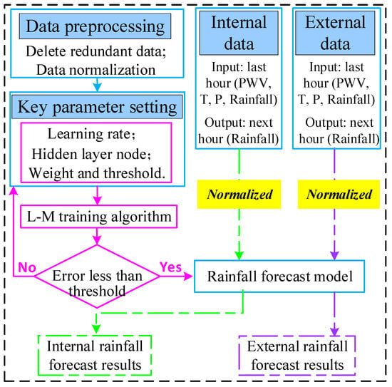
Figure 2.
General flowchart of establishing short-term rainfall forecast model based on the BP-NN algorithm using GNSS observations.
3.3.2. Determination of Key Parameters for the BP-NN Algorithm
By considering the drawbacks of the traditional BP-NN algorithm, such as slow convergence, susceptibility to local minima, and training paralysis, the Levenberg–Marquardt (L-M) training algorithm was introduced to improve the weight correction method of BP-NN [35]:
where is the corrected weight of the L-M algorithm, is the Jacobian matrix of the derivative of the network error to the weight, is the error vector, and is a scalar—when is 0, the L-M equation uses the Newton method, and when is larger, the L-M equation uses the gradient method. The improved L-M method has two advantages compared with the traditional BP-NN algorithm. Firstly, the L-M method has an extremely fast convergence speed. Secondly, this method combines the advantages of the gradient descent and Newton methods, and its performance is considerably more stable than the traditional algorithm.
The number of hidden layer nodes and the learning rate are two key parameters that determine the forecast accuracy of the BP-NN algorithm. Choosing an appropriate method to determine these parameters is a key step in building the BP-NN model. If the number of hidden layer nodes is too small, then the overall convergence speed of the neural network will slow down and it is easy to fall into local minima. Similarly, having too few hidden layer nodes limits the ability of the BP-NN to establish complex decision boundaries, resulting in difficulty in training the BP-NN or in recognizing new samples, and a reduced fault tolerance. However, if the number of hidden layer nodes is too high, this will lead to a long learning time and reduced generalization ability of the BP-NN model. In this study, the optimal number of hidden layer nodes is determined based on the Kolmogorov theorem. The equivalent relationship between the numbers of input and hidden layer neurons is as follows [35]:
where are the numbers of nodes in the hidden and input layers, respectively. The number of hidden layer nodes selected according to the Kolmogorov theorem can accurately express any mapping and make the hidden layer capacity and training time coordinate with each other.
The selection of the learning rate has always been an issue with the BP-NN algorithm. If the learning rate chosen is too small, then, while it can ensure the convergence of the neural network, it requires numerous iterations, resulting in slow convergence. Conversely, f the learning rate chosen is too large, then it may lead to over-correction, resulting in the neural network struggling to converge [36]. Therefore, the learning rate is determined based on the following empirical formula proposed by Kung and Hwang [37]:
where and are the learning rate and number of hidden layer nodes, respectively.
3.4. Evaluation Index
To allow comparison with previous studies [11,17], the TDR and FFR are selected as evaluation indexes for the proposed rainfall forecast model. The specific calculation formulas for the TDR and FFR are as follows:
where refers to the correct number of model rainfall forecasts, refers to the number of actual occurrences of rainfall, and refers to the false number of model rainfall forecasts.
4. Result and Discussion
4.1. Validation of the GNSS-Derived ZTD
The pressure, temperature, and PWV data provided by ERA5 are used to calculate ZTD at the four selected GNSS stations, which is used to evaluate the accuracy of the GNSS-derived ZTD. Figure 3 shows the distribution of the ZTD probability density calculated by GNSS and ERA5 at the four stations (G01, G02, GZ3, and T01) across the whole of 2021. It can be observed that the GNSS-derived and ERA5-provided ZTD have good consistency. The correlation coefficients between the GNSS-derived and ERA5-provided ZTD at the four stations are all as high as 0.97. The statistical results show that the average RMS and bias of ZTD at the 15 GNSS stations in the experimental area for the whole of 2021 are 16.8 mm and −7.1 mm, respectively. This result indicates that the derivation of ZTD from GNSS observations has good performance.
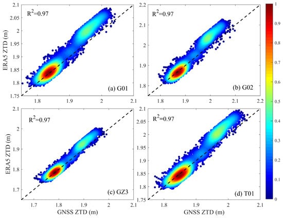
Figure 3.
Distribution of the ZTD probability density calculated using GNSS observations and ERA5 data across the whole of 2021.
4.2. Validation of the Regional High-Precision Tm Model
Four models are compared to evaluate the accuracy of the proposed regional Tm model. Model 1 considers only the periodic term. Model 2 considers the periodic term and T. Model 3 considers the periodic term, T, and P. The Tm model developed in this study is called RTm. The Tm data calculated from four models are obtained from 2020 to 2021 and compared with the Tm values obtained from five radiosonde stations as the real values. Figure 4 shows the statistical results for each model at the five radiosonde stations. It can be found that the Tm model (RTm) considering multiple meteorological and periodic factors has higher accuracy than the other Tm models. This result confirms the correlation between Tm and multiple meteorological factors. Moreover, this result verifies the good performance of the regional model established under the conditions of multiple meteorological factors. The Tm model, including temperature (Model 2), also has significantly better performance than the Tm model considering only annual and semi-annual periods (Model 1). This outcome indicates that the model is significantly affected by temperature. The accuracy of the Tm model only slightly improved after also considering pressure and relative humidity, indicating that the impact of these meteorological factors on this model is limited. Lastly, the regional Tm model proposed in this study has better performance than previous Tm models.
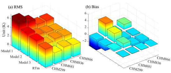
Figure 4.
Validation of the different Tm models from 2020 to 2021.
Nine representative Tm models are selected to further validate the accuracy of the proposed RTm model: GTm-I [28], GTm-H [29], GTrop [38], GPT2w [32], IGPT2w [39], GPT3 [33], CTm [40], NNTm [41], and Bevis [25]. Figure 5 shows the comparison results of different models in calculating Tm and the Tm derived from the data from the five radiosonde stations from 2020 to 2021. As can be seen, the RTm model has the highest accuracy and good stability in the study area. Table 3 presents the specific statistical results of the 10 models, which reveal, while that the RMS of the CTm and RTm models are both below 3 K, the RTm model is still superior to the CTm model.
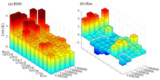
Figure 5.
Comparison of the performance of 10 Tm models.

Table 3.
Comparison of the accuracy of 10 Tm models at 12 RS stations from 2020 to 2021.
4.3. Validation of the GNSS-Derived PWV
The ERA5-provided PWV is selected to evaluate the performance of the GNSS-derived PWV. Figure 6 shows the comparison of the long time series of PWV at the four selected GNSS stations between GNSS and ERA5 over the whole of 2021. It can be observed that the GNSS-derived and ERA5-provided PWV follow the same trend and have a high degree of agreement, with a correlation coefficient exceeding 0.97. The statistical results show that the average RMS/bias/MAE of the four stations are 3.99/−1.08/2.84 mm, respectively, with the G02 station having the largest deviation with RMS/Bias/MAE of 4.33/−2.05/3.24 mm, and the GZ3 station having the smallest deviation with RMS/Bias/MAE of 2.64/−0.71/2.12 mm. These results show that the GNSS-derived PWV using the PPP technique has good accuracy.
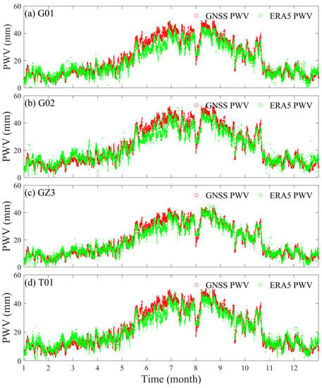
Figure 6.
Long time series GNSS-derived and ERA5-provided PWV at four GNSS stations for the whole of 2021.
4.4. Validation of the Rainfall Forecast Model Using the BP-NN Algorithm
The input parameters of the rainfall forecast model based on the BP-NN algorithm are PWV, T, P, and rainfall data. The corresponding number of input nodes is 4. According to the theory introduced in Section 3.3, the number of hidden layer nodes and learning rate for establishing the rainfall forecast model are determined to be 9 and 0.2, respectively, and there is a single output node. Therefore, the basic structure of the rainfall forecast model constructed by the BP-NN algorithm in this experiment is 4-9-1. The activation functions for the output and hidden layer nodes of the BP-NN are ReLU and Sigmoid, respectively. The weights and thresholds of the BP-NN model initialization are randomly generated based on the Nguyen–Widrow algorithm. Moreover, the L-M optimization weight method is used to optimize the BP-NN model. Considering that the experiment aims to forecast whether rainfall will occur in the next hour, rainfall intensity and duration are not forecast. Therefore, the observed and simulated/forecasted rainfall events are binarized.
- (1)
- Determination of the rainfall threshold
The simulated output of the rainfall forecast model can be negative and fluctuate around 0 mm. Hence, an accurate threshold is required to determine the simulated rainfall threshold. The rainfall threshold in this study is determined based on the highest TDR and lowest FFR of the rainfall forecast model using the BP-NN algorithm. The method for determining the rainfall threshold is to set an initial variable N, and set simulated rainfall values less than or equal to N mm to 0 mm, and simulated rainfall values greater than N mm to 1 mm. Thus, the range of the variable N is 0–1 mm. Figure 7 shows the results of the simulated and forecast TDR and FFR for the spring rainfall in 2021 under different rainfall threshold settings for scheme 1, where Figure 7a,b show the simulated rainfall forecast results and external rainfall forecast results, respectively. It can be seen that as the rainfall threshold N increases, the TDR decreases and the FFR increases. In addition, the trend in the forecast experiment is similar to that in the simulated experiment. The TDR and FFR also decrease as the threshold increases. Therefore, the rainfall threshold for the simulated and forecast rainfall events is 0 mm according to the selection principle of the rainfall threshold with the highest TDR and lowest FFR. Furthermore, the corresponding accuracies of the proposed rainfall forecasting model are the highest, at 97.53%/2.48% and 96.30%/42.22%, respectively.
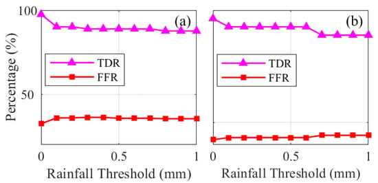
Figure 7.
Rainfall simulation and forecast threshold selection based on the BP-NN algorithm, where (a) is the simulation experiment and (b) is the forecast experiment.
- (2)
- Simulated result of the rainfall forecast model
The simulated result of the remaining schemes is obtained using the preceding method for determining rainfall threshold values. Figure 8 shows the TDR and FFR of different schemes for different seasons over the whole of 2021. It can be seen that the TDR of all schemes is the same for different seasons (i.e., over 95%). In addition, the FFR is below 50%. The FFR in the winter is also higher than that in other seasons across all the schemes. Such a result indicates that the accuracy of the BP-NN algorithms in winter rainfall forecasting is lower than that in other seasons. In addition, it should be noted that the FFR values of schemes 3 and 4 are significantly lower than those of schemes 1 and 2. This result indicates that schemes 3 and 4 have higher accuracy than schemes 1 and 2. The simulated rainfall results for the four schemes based on the BP-NN model show that the TDR is similar among different schemes, while the FFR differs significantly among the schemes. Statistical results show that the average TDR and FFR for the four schemes are 94.6% and 42.1%, respectively. This outcome indicates that the simulated accuracy of the model constructed based on the BP-NN algorithm is consistent with the expected experimental results and can be further applied to forecast experiments.
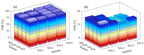
Figure 8.
TDR and FFR for rainfall forecasting under different seasons for the four schemes, where (a) and (b) are the TDR and FFR of proposed rainfall forecasting model, respectively.
- (3)
- Forecast result of the rainfall forecast model
To further validate the accuracy of the proposed short-term rainfall forecast model based on the BP-NN algorithm, Figure 9 presents the TDR and FFR of the four experimental schemes for rainfall forecast in different seasons. The results show that the lowest TDR of rainfall warning occurred in the summer of scheme 2, with a value of only 89.47%, and the highest TDR occurred in the spring and winter of scheme 2, both of which are 100%. However, the FFR for each scheme and season exhibited a highly random phenomenon, with the highest value occurring in the spring of scheme 2 and the lowest value occurring in the summer of scheme 3 (48.14% and 26.93%, respectively). These results indicate that the short-term rainfall forecast model based on the BP-NN algorithm has good adaptability among different seasons and schemes and can achieve good rainfall forecast accuracy. The statistical results show that the average TDR and FFR of the constructed rainfall forecast model are 93.70% and 38.30%, respectively. This result further verifies the performance and applicability of the proposed rainfall forecast model in landslide-prone areas.
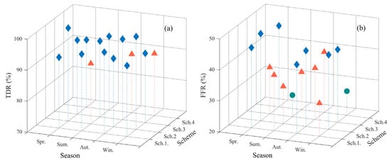
Figure 9.
TDR and FFR accuracy of rainfall forecasting for the four schemes in the forecasting experiments on a seasonal scale ((a): 80–90%: orange triangle; 90–100%: blue diamond; (b): 20–30%: green circle; 30–40%: orange triangle; 40–50%: blue diamond).
4.5. Discussion
It can be concluded from Figure 4 and Table 3 that the proposed RTm model has better performance than other typical empirical Tm models. This indicates that Tm is affected by multiple meteorological factors, and also has regional characteristics, therefore, those two aspects should both be considered when establishing a high-precision Tm model. At the same time, it should be noted that this method is only suitable for regional Tm modeling with high precision, as a global Tm model cannot be well-described by local parameters.
Compared to GNSS-derived PWV, ERA5-provided PWV is an underestimate when PWV levels are high (Figure 6). This is because the ERA5-provided PWV is a numerical assimilation result and cannot accurately capture small-scale extreme weather changes. In addition, it can be found that the PWV difference is largest from June to August for those stations, this is because June to August corresponds to the Summer, and levels of atmospheric water are larger in Summer than in other seasons. Therefore, the difference in PWV between GNSS and ERA5 is slightly larger during this period.
Although the TDR of the proposed rainfall forecasting model can reach up to 93% while the FFR is lower than 40%, it should be noted that the TDR and FFR are slightly different for different schemes. This is because the input data for training the different rainfall forecasting models are different, and the established models are not exactly the same due to the training data being different. Therefore, working out how to obtain high-quality and extensive training data for the BP-NN algorithm is very important to establish a stable rainfall forecasting model. In addition, it also can be seen that the proposed model has poorer performance in winter due to the occurrence of less rainfall in this season.
5. Conclusions
To overcome the limitations of traditional numerical forecasting in forecasting rainfall on the small spatial scale of landslide-prone areas, this study proposes a short-term rainfall forecast model that combines the BP-NN algorithm and GNSS observations. To obtain high-precision GNSS-derived PWV, the Tm model of the study area is first established using data from 12 radiosonde stations. Thereafter, the rainfall forecast model based on the BP-NN algorithm is trained using parameters such as PWV, temperature, and pressure obtained from GNSS and meteorological stations. The trained model is then used to forecast rainfall in the next hour. The proposed method is validated using data from four selected GNSS stations and the corresponding meteorological parameters in a landslide-prone area located in Yunnan Province, China. Experimental results show that the established regional Tm model has high accuracy, with the average RMS and bias of 3 K and 0.15 K, respectively. Moreover, the evaluation of the short-term rainfall forecast model based on the BP-NN algorithm shows that the TDR of the simulation and measurement for the four studied schemes are over 95%, while the FFR is under 40%. Such results show that the proposed rainfall forecast model has high rainfall forecast accuracy and provides a new method for short-term rainfall forecast in landslide-prone areas.
Author Contributions
Conceptualization, Z.L., Y.M. and Y.L.; methodology, Z.L. and Q.Z.; software, Z.L., Y.L. and Y.M.; validation, Z.L., Y.L., W.R. and J.L.; writing—original draft preparation, Z.L., Y.M., J.L. and Y.L.; writing—review and editing, Y.M., J.L. and Q.Z.; visualization, Z.L., Y.L., Y.M. and W.R. All authors have read and agreed to the published version of the manuscript.
Funding
The research was funded by the Science and technology projects of Northwest Engineering Corporation Limited (XBY-2016-10, XBY-KJ-2019-06, and XBY-KJ-2021-14), the Open Fund Project of National Dam Safety Engineering Technology Research Center (CX2022B01) and the local special scientific research plan project of Shaanxi Provincial Department of Education (22JE012), National Natural Science Foundation of China (42274039) and Shaanxi Provincial Innovation Capacity Support Plan Project (2023KJXX-050).
Institutional Review Board Statement
Not applicable.
Informed Consent Statement
Not applicable.
Data Availability Statement
The data can be obtained by contacting the corresponding author.
Acknowledgments
Thanks to the ECMWF for providing the corresponding meteorological data and the IGRA for providing the Radiosonde data.
Conflicts of Interest
The authors declare no conflict of interest.
References
- Le Breton, M.; Bontemps, N.; Guillemot, A.; Baillet, L.; Larose, É. Landslide monitoring using seismic ambient noise correlation: Challenges and applications. Earth Sci. Rev. 2021, 216, 103518. [Google Scholar] [CrossRef]
- Liu, Y.; Qiu, H.; Yang, D.; Liu, Z.; Ma, S.; Pei, Y.; Zhang, J.; Tang, B. Deformation responses of landslides to seasonal rainfall based on InSAR and wavelet analysis. Landslides 2022, 19, 199–210. [Google Scholar] [CrossRef]
- Abraham, M.T.; Satyam, N.; Bulzinetti, M.A.; Pradhan, B.; Pham, B.T.; Segoni, S. Using field-based monitoring to enhance the performance of rainfall thresholds for landslide warning. Water 2020, 12, 3453. [Google Scholar] [CrossRef]
- Moya-Álvarez, A.S.; Martínez-Castro, D.; Kumar, S.; Estevan, R.; Silva, Y. Response of the WRF model to different resolutions in the rainfall forecast over the complex Peruvian orography. Theor. Appl. Climatol. 2019, 137, 2993–3007. [Google Scholar] [CrossRef]
- Ma, Y.; Chandrasekar, V.; Chen, H.; Cifelli, R. Quantifying the potential of AQPI gap-filling radar network for streamflow simulation through a WRF-hydro experiment. J. Hydrometeorol. 2021, 22, 1869–1882. [Google Scholar] [CrossRef]
- Pal, S.; Dominguez, F.; Dillon, M.E.; Alvarez, J.; Garcia, C.M.; Nesbitt, S.W.; Gochis, D. Hydrometeorological observations and modeling of an extreme rainfall event using WRF and WRF-hydro during the RELAMPAGO field campaign in Argentina. J. Hydrometeorol. 2021, 22, 331–351. [Google Scholar] [CrossRef]
- Li, H.; Choy, S.; Wang, X.; Liang, H.; Zhang, K. Monitoring the Migration of Water Vapor Using Ground-Based GNSS Tropospheric Products. IEEE Geosci. Remote Sens. Lett. 2023. [Google Scholar] [CrossRef]
- Manandhar, S.; Dev, S.; Lee, Y.H.; Meng, Y.S.; Winkler, S. A data-driven approach to detecting precipitation from meteorological sensor data. In Proceedings of the IGARSS 2018–2018 IEEE International Geoscience and Remote Sensing Symposium, Valencia, Spain, 22–27 July 2018; pp. 3872–3875. [Google Scholar]
- Benevides, P.; Catalao, J.; Miranda, P.M.A. On the inclusion of GPS precipitable water vapour in the nowcasting of rainfall. Nat. Hazards Earth Syst. Sci. 2015, 15, 2605–2616. [Google Scholar] [CrossRef]
- Zhao, Q.; Liu, Y.; Ma, X.; Yao, W.; Yao, Y.; Li, X. An Improved Rainfall Forecasting Model Based on GNSS Observations. IEEE Trans. Geosci. Remote Sens. 2020, 58, 4891–4900. [Google Scholar] [CrossRef]
- Li, H.; Choy, S.; Zaminpardaz, S.; Carter, B.; Sun, C.; Purwar, S.; Liang, H.; Li, L.; Wang, X. Investigating the Inter-Relationships among Multiple Atmospheric Variables and Their Responses to Precipitation. Atmosphere 2023, 14, 571. [Google Scholar] [CrossRef]
- Li, H.; He, Y.; Xu, Q.; Deng, J.; Li, W.; Wei, Y. Detection and segmentation of loess landslides via satellite images: A two-phase framework. Landslides 2022, 19, 673–686. [Google Scholar] [CrossRef]
- Li, H.; He, Y.; Xu, Q.; Deng, J.; Li, W.; Wei, Y.; Zhou, J. Sematic segmentation of loess landslides with STAPLE mask and fully connected conditional random field. Landslides 2023, 20, 367–380. [Google Scholar] [CrossRef]
- Hashim, F.R.; Daud, N.N.; Ahmad, K.A.; Adnan, J.; Rizman, Z.I. Prediction of rainfall based on weather parameter using artificial neural network. J. Fundam. Appl. Sci. 2017, 9, 493–502. [Google Scholar] [CrossRef]
- Srivastava, T.; Kumar, P.; Singh, B.P. Rainfall Forecast of Kumarganj area using artificial neural network (ANN) models. Soc. Sci. Dev. Agric. Technol. Meerut(U. P.) INDIA 2017, 12, 1375–1379. [Google Scholar]
- Guan, Z.; Tian, Z.; Xu, Y.; Dai, H. Rainfall predict and comparing research based on Arcgis and BP neural network. 2016 3rd International Conference on Materials Engineering. Manuf. Technol. Control. 2016. [Google Scholar] [CrossRef]
- Benevides, P.; Catalao, J.; Nico, G. Neural Network Approach to Forecast Hourly Intense Rainfall Using GNSS Precipitable Water Vapor and Meteorological Sensors. Remote Sens. 2019, 11, 966. [Google Scholar] [CrossRef]
- Li, H.; Wang, X.; Zhang, K.; Wu, S.; Xu, Y.; Liu, Y.; Qiu, C.; Zhang, J.; Fu, E.; Li, L. A neural network-based approach for the detection of heavy precipitation using GNSS observations and surface meteorological data. J. Atmos. Sol. Terr. Phys. 2021, 225, 105763. [Google Scholar] [CrossRef]
- Petit, G.; Luzum, B. IERS Conventions. IERS Tech. Note 2010, 36, 1–95. [Google Scholar]
- Durre, I.; Vose, R.S.; Wuertz, D.B. Overview of the integrated global radiosonde archive. J. Clim. 2006, 19, 53–68. [Google Scholar] [CrossRef]
- Campanelli, M.; Nakajima, T.; Khatri, P.; Takamura, T.; Uchiyama, A.; Estelles, V.; Liberti, G.L.; Malvestuto, V. Retrieval of characteristic parameters for water vapour transmittance in the development of ground-based sun–sky radiometric measurements of columnar water vapour. Atmos. Meas. Tech. 2014, 7, 1075–1087. [Google Scholar] [CrossRef]
- Herring, T.A.; King, R.W.; McClusky, S.C. Introduction to GAMIT/GLOBK, 10.4. Massachusetts Institute of Technology: Cambridge, MA, USA.
- Li, X.; Dick, G.; Ge, M.; Heise, S.; Wickert, J.; Bender, M. Real-time GPS sensing of atmospheric water vapor: Precise point positioning with orbit, clock, and phase delay corrections. Geophys. Res. Lett. 2014, 41, 3615–3621. [Google Scholar] [CrossRef]
- Saastamoinen, J. Contributions to the theory of atmospheric refraction. Bull. Géodésique 1972, 105, 279–298. [Google Scholar] [CrossRef]
- Bevis, M.; Businger, S.; Herring, T.A.; Rocken, C.; Anthes, R.A.; Ware, R.H. GPS meteorology: Remote sensing of atmospheric water vapor using the global positioning system. J. Geophys. Res. 1992, 97, 15787. [Google Scholar] [CrossRef]
- Yao, Y.; Zhang, B.; Xu, C.; Yan, F. Improved one/multi-parameter models that consider seasonal and geographic variations for estimating weighted mean temperature in ground-based GPS meteorology. J. Geod. 2014, 88, 273–282. [Google Scholar] [CrossRef]
- Bevis, M.; Businger, S.; Chiswell, S.; Herring, T.A.; Anthes, R.A.; Rocken, C.; Ware, R.H. GPS meteorology: Mapping zenith wet delays onto precipitable water. J. Appl. Meteorol. 1994, 33, 379–386. [Google Scholar] [CrossRef]
- Yao, Y.B.; Zhang, B.; Yue, S.Q.; Xu, C.Q.; Peng, W.F. Global empirical model for mapping zenith wet delays onto precipitable water. J. Geod. 2013, 87, 439–448. [Google Scholar] [CrossRef]
- YAO, Y.; SUN, Z.; XU, C.; XU, X. Global Weighted Mean Temperature Model Considering Nonlinear Vertical Reduction. Geomat. Inf. Sci. Wuhan Univ. 2019, 44, 106–111. [Google Scholar]
- Böhm, J.; Heinkelmann, R.; Schuh, H. Short note: A global model of pressure and temperature for geodetic applications. J. Geod. 2007, 81, 679–683. [Google Scholar] [CrossRef]
- Lagler, K.; Schindelegger, M.; Böhm, J.; Krásná, H.; Nilsson, T. GPT2: Empirical slant delay model for radio space geodetic techniques. Geophys. Res. Lett. 2013, 40, 1069–1073. [Google Scholar] [CrossRef]
- Böhm, J.; Möller, G.; Schindelegger, M.; Pain, G.; Weber, R. Development of an improved empirical model for slant delays in the troposphere (GPT2w). GPS Solut. 2015, 19, 433–441. [Google Scholar] [CrossRef]
- Landskron, D.; Böhm, J. VMF3/GPT3: Refined discrete and empirical troposphere mapping functions. J. Geod. 2018, 92, 349–360. [Google Scholar] [CrossRef] [PubMed]
- Lee, S.-W.; Choi, B.I.; Woo, S.-B.; Kim, J.C.; Kim, Y.-G. Calibration of a radiosonde humidity sensor at low temperature and low pressure. Metrologia 2019, 56, 055008. [Google Scholar] [CrossRef]
- Yu, Y. Intelligent Reliability Analysis with Incomplete Covariates; Queensland University of Technology: Brisbane, Queensland, 2012. [Google Scholar]
- Yu, F.; Xu, X. A short-term load forecasting model of natural gas based on optimized genetic algorithm and improved BP neural network. Appl. Energy 2014, 134, 102–113. [Google Scholar] [CrossRef]
- Kung, S.Y.; Hwang, J.N. An Algebraic Projection Analysis for Optimal Hidden Units Size and Learning Rates in Back-Propagation Learning. Proc. IEEE Int. Conf. Neural Netw. 1988, 1, 363–370. [Google Scholar]
- Sun, Z.; Zhang, B.; Yao, Y. A global model for estimating tropospheric delay and weighted mean temperature developed with atmospheric reanalysis data from 1979 to 2017. Remote Sens. 2019, 11, 1893. [Google Scholar] [CrossRef]
- Huang, L.; Liu, L.; Chen, H.; Jiang, W. An improved atmospheric weighted mean temperature model and its impact on GNSS precipitable water vapor estimates for China. GPS Solut. 2019, 23, 51. [Google Scholar] [CrossRef]
- Huang, L.; Peng, H.; Liu, L.; Li, C.; Kang, C.; Xie, S. An empirical atmospheric weighted mean temperature model considering the lapse rate function for China. Acta Geod. Et Cartogr. Sin. 2020, 49, 432–442. [Google Scholar]
- Ding, M. A neural network model for predicting weighted mean temperature. J. Geod. 2018, 92, 1187–1198. [Google Scholar] [CrossRef]
Disclaimer/Publisher’s Note: The statements, opinions and data contained in all publications are solely those of the individual author(s) and contributor(s) and not of MDPI and/or the editor(s). MDPI and/or the editor(s) disclaim responsibility for any injury to people or property resulting from any ideas, methods, instructions or products referred to in the content. |
© 2023 by the authors. Licensee MDPI, Basel, Switzerland. This article is an open access article distributed under the terms and conditions of the Creative Commons Attribution (CC BY) license (https://creativecommons.org/licenses/by/4.0/).