Carbon Emission Model and Emission Reduction Technology in the Asphalt Mixture Mixing Process

Abstract

This paper attempts to develop a calculation model to estimate the carbon dioxide (CO₂) emissions during the mixing process of asphalt mixtures and explore energy-saving and emission reduction technologies. Based on a comprehensive analysis of the mixer’s working mechanism, mixing quality requirement, and theoretical deductions, a CO₂ emission model for the mixing process of asphalt mixtures is established. The model highlights the significant impact of mixing time on both mixing quality and carbon emissions. The model demonstrates that the mixing quality improves with an increase in mixing time, but the degree of improvement diminishes after an initial significant enhancement, eventually stabilizing. Importantly, excessive mixing time does not significantly improve the mixing quality; conversely, an extended mixing time has a notable impact on carbon emissions. Results show that when the deviation of the asphalt content is changed from 0.3% to 0.2% for a 5% asphalt content mixture, the mixing time and resulting CO₂ emissions increase by 14%; similarly, when the deviation is 0.1%, the mixing time and resulting CO₂ emissions increase by nearly 40%. Additionally, the agitator’s capacity also significantly influences the CO₂ emissions. For a project of a given scale, increasing the agitator capacity leads to a reduction in total carbon emissions during the mixing process. Compared to a type 1500 agitator, employing agitators of types 3000, 4000, and 5000 can achieve reductions in total CO₂ emissions by 26.3%, 32.9%, and 36.8%, respectively. Therefore, for large-scale engineering projects aiming to minimize CO₂ emissions during the mixing process, it is essential to determine the optimal mixing time to avoid excessive mixing and select a larger capacity agitator, preferably type 4000 or higher. These findings could support the development of effective emission reduction measures in the field of road construction, thereby contributing to the achievement of emission reduction targets and promoting the advancement of sustainable road development.

1. Introduction

The increasing influence of global warming on our daily lives has led to a growing concern about carbon emissions in various fields of study, particularly concerning the implementation of various effective energy-saving and emission reduction measures. The transportation sector stands out as a significant contributor to global carbon emissions, accounting for approximately 24% of the worldwide energy-related carbon emissions in 2020 [1]. As a main part of the transportation infrastructure, roads are developing rapidly in China resulting in increasing carbon emissions. In the future, the total mileage of roads will continue to increase and the number of maintenance activities will also increase. This will further lead to a rapid increase in carbon emissions, which will conflict with the goal of achieving carbon neutrality in the transportation sector. However, carbon emissions from energy consumption and material production during road construction have not been accurately quantified until recently [2,3].

In transportation infrastructure construction, asphalt mixtures are the most commonly used materials for constructing roads, bridges and airfields worldwide. The manufacturing of mixture, transporting to the job site, and the paving and rolling processes involved in asphalt road construction will consume significant amounts of fuels and electricity, leading to massive greenhouse gases emissions [4]. With the rapid development of infrastructure, this elevated energy demand profoundly influences the social and economic development of the country. There is a growing concern regarding the environmental impact, and numerous studies have been devoted to assessing the carbon emissions associated with asphalt road construction and exploring the emission reduction technologies.

Many scholars have employed the life cycle assessment (LCA) method to analyze carbon emissions from road construction projects and develop integrated models for estimating emissions in asphalt road construction and for preventive maintenance, rehabilitation, and reconstruction [5,6,7]. These studies encompass carbon emissions at various stages, including material production, on-site road construction, mixture production, and transportation. Some studies aim to estimate the level of emissions and identify the major emission sources. For instance, Liu et al. [8] estimated and compared the magnitude of carbon dioxide (CO₂) emissions of 20 asphalt road projects and 18 concrete roads, revealing that asphalt road construction activities generated twice the total CO₂ emissions compared to concrete road construction. Garraín and Lechón [9] presented a method to evaluate CO₂ emissions for asphalt pavement rehabilitation. The material production phase was identified as the most significant source of carbon emissions for newly constructed roads, reconstruction projects, and road rehabilitation [9,10,11,12,13].

Compared to other on-site construction activities, the manufacturing of asphalt mixtures contributes a higher percentage of carbon emissions [9,14]. These studies emphasize the significance of the material production process when assessing carbon emissions throughout the entire life cycle of asphalt roads. Several studies have established models to analyze the energy consumption and carbon emissions during asphalt mixture production. Asphalt mixtures are produced in asphalt plants, where the fuel for the burner to heat materials and the electricity for the plant to operate are dominant sources of emissions [15,16]. Dos Santos et al. [17] quantified emissions and evaluated energy consumption during the drying and heating of aggregates in dryer drums in different asphalt plants. Thives and Ghisi [18] analyzed the factors affecting emissions and reported that aggregate moisture content, manufacture temperature and fuel type are major factors. Paranhos and Petter [16] presented a comprehensive multivariate data analysis dedicated to analyzing the emissions from hot-mix asphalt (HMA) plants when heating and drying mixtures. Furthermore, Chong et al. [19] also considered the electricity consumption of plant operation based on rated power and operating period, but did not analyze specific factors affecting electricity consumption.

In terms of emissions reduction, several specific studies have been published concerning emission reduction measures during asphalt mixture production [18,20]. Most of them identified the use of recycled materials, such as reclaimed asphalt pavement (RAP), and new manufacturing techniques like warm-mix asphalt (WMA) and cold recycling techniques as preferred options for reducing emissions [21,22,23,24,25,26]. For example, Rodriguez-Alloza et al. [24] pointed out that WMA can reduce the temperature required for producing and placing materials, resulting in a 20% reduction in CO₂ emissions compared to traditional HMA. Giani et al. [27] carried out a comparison of traditional techniques and cold-in-place recycling techniques with the application of RAP, where the latter could decrease about 12% of CO₂ emissions and 15% of energy consumption. In addition, Rubio et al. [15] compared emissions from different types of plants and generally found that conventional discontinuous plants (batch asphalt plants) emitted more carbon emissions than continuous plants (drum asphalt plants).

Current studies have primarily focused on the emission characteristics of entire construction projects and on emission mitigation strategies from a relatively macro perspective. Studies related to asphalt mixture production primarily analyze direct on-site emissions from the heating and drying of materials in the dryer drum. However, it is important to note that the material mixing process also consumes electricity and produces associated embodied carbon emissions from a life cycle perspective. The omission of such carbon emissions may lead to an underestimation of the emission level from asphalt mixture production during road construction. Moreover, there is a lack of refined quantitative analysis of carbon emissions within specific construction processes, particularly in the context of the asphalt mixing process, considering comprehensive factors, such as equipment structure, materials characteristics, and technique mechanisms.

Therefore, the primary objectives of this study are to develop an integrated model for estimating energy consumption and carbon emissions during the asphalt mixing process, to identify key factors influencing emissions, and to explore optimal mixing conditions and approaches for reducing energy consumption and carbon emissions in road construction. To achieve these goals, a commonly used batch asphalt plant equipped with a twin-shaft pugmill agitator (TSPA) is used for analysis. We established the correlations between agitator design parameters, operational parameters, and carbon emissions in order to investigate techniques and methods for emission reduction. This study will contribute to the understanding of life cycle carbon emissions in the mixing process. The findings could support the development of effective emission reduction measures and sustainable road construction practices, contributing to efforts to combat climate change.

2. Analysis Boundary and Mixing Mechanism

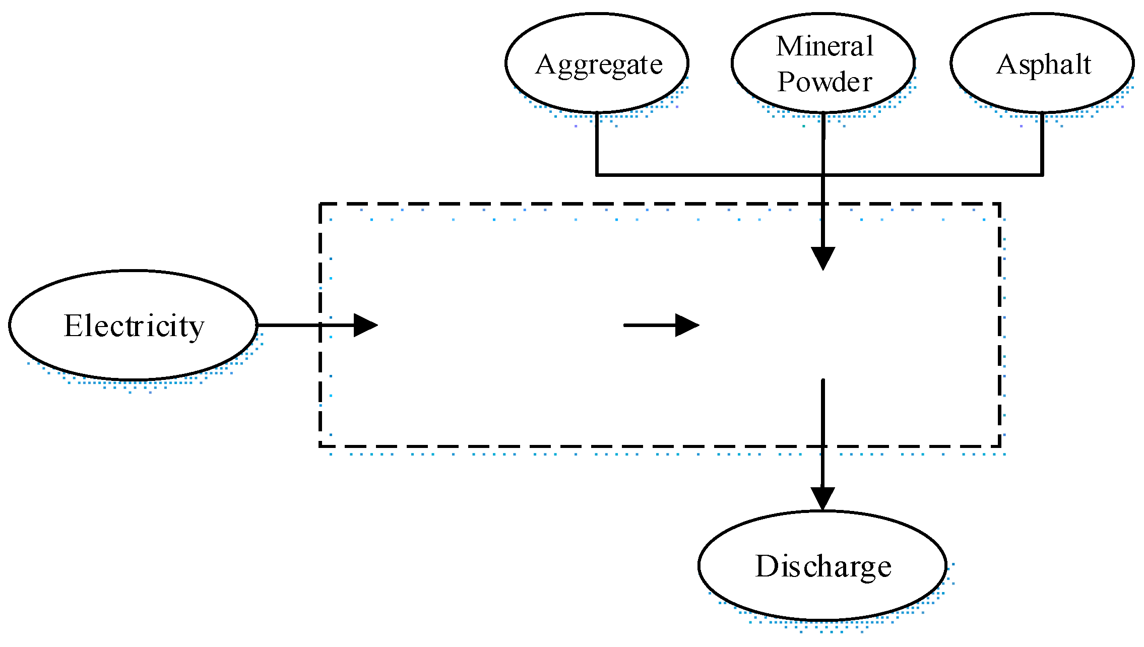
2.1. Analysis Boundary

In the road construction sector, the asphalt mixture plant is one of the most important equipment, and is responsible for the production of the mixture. Its primary function is to mix coarse and fine aggregates, asphalt binders, mineral fillers, and other additives into a uniform mixture at a certain temperature. The production process in the plant typically consists of providing cold aggregates from storage bins in a controlled amount, subsequently heating and drying them in the dryer drum, vibrating them in a screen deck, and mixing aggregates with the heated and injected asphalt in a mixer. This equipment comprises several components, including a batching system, a drying and heating system, a vibrating screening system, a metering system, a mixer, an induced air dust removal system, and a control system. Notably, the mixer is the main component of the asphalt mixture plant, as it allows materials to be mixed in it [28]. To establish a clear scope of analysis, it is important to define the system boundary. This study focuses on analyzing the carbon emissions during the mixing process that occurs within a mixer. The carbon emissions come from the consumption of electrical sources, which are used for energy to operate the mixer. The mixer consists of a motor and an agitator. The analysis boundary is depicted in Figure 1. The analysis aims to examine influencing factors and calculate carbon emissions generated during the mixing process. Indirect links, such as equipment processing, manufacturing, and installation, are excluded from the analysis.

This study aims to provide a method to quantify the energy consumption of the mixing process and its impact on climate change. Six greenhouse gases (GHGs) contributing to climate change are defined by the Kyoto Protocol, including carbon dioxide (CO₂), nitrous oxide (N₂O), methane (CH₄), hydrofluorocarbons (HFC), perfluorocarbons (PFC), and sulfur hexafluoride (SF₆). The first three GHGs are mainly associated with electricity production. Particularly, CO₂ emission is analyzed in this study due to its critical role in global climate change. CO₂ accounts for 77% of total GHGs, and its concentration continues to rise, leading to global warming [29]. Therefore, studying CO₂ emissions is essential for understanding the mechanisms of climate change and implementing mitigation measures. Additionally, studying CO₂ emissions can also help to infer the emissions and changes in other GHGs.

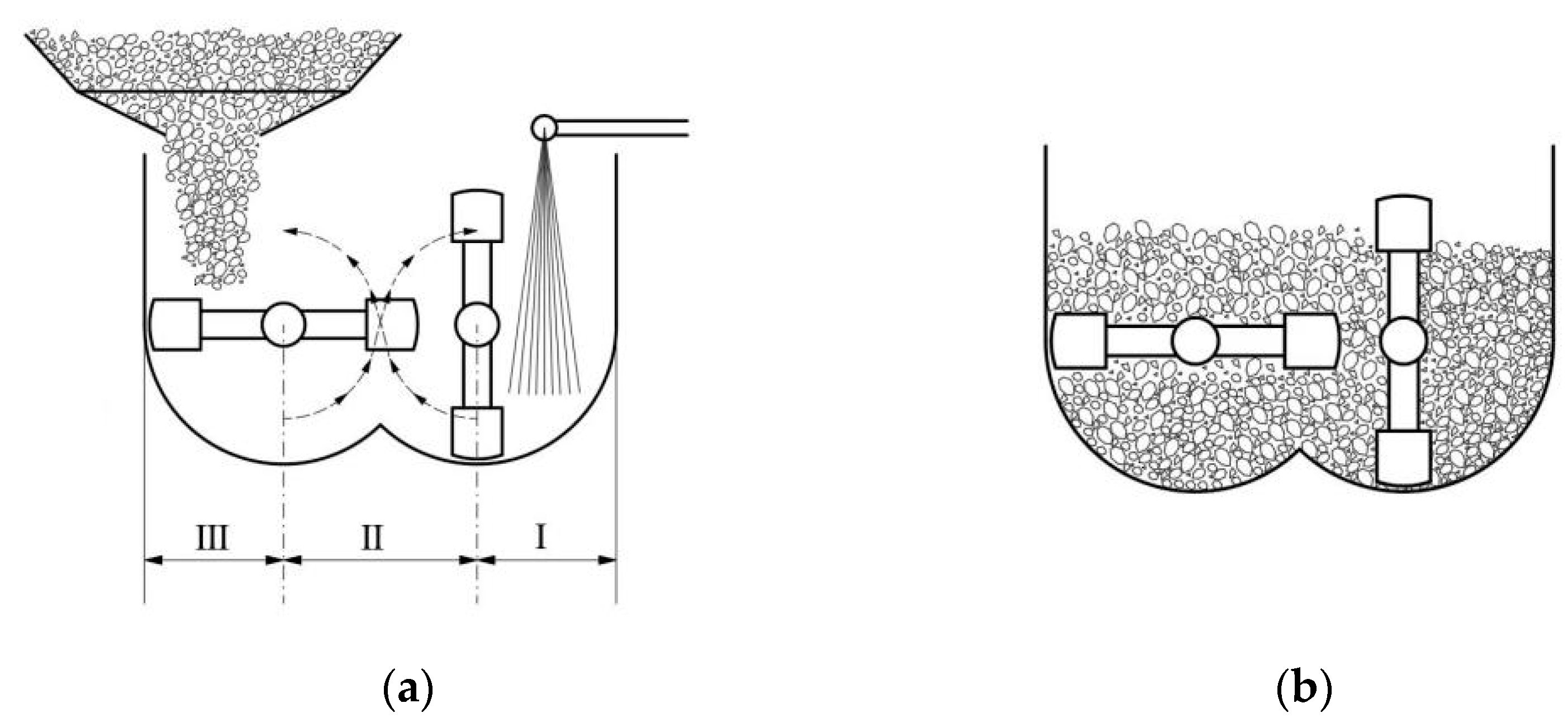
2.2. Structure of the Mixer

A mixer equipped with a twin-shaft pugmill agitator is commonly used. It is composed of a driving motor, a cylinder, an agitator shaft, an agitator arm, an agitator blade, a synchronizer, and a discharge gate. The structure is shown in Figure 2. The agitator blade is installed at the end of the mixing arm, set at an angle of 45° with respect to the mixing shaft. It maintains gaps of 4 mm and 6 mm from the cylinder liner. The arms are fixed to the shaft, and the two shafts are driven by the motor. The synchronizer ensures that the rotation of the two shafts remains synchronized, enabling efficient mixing of the asphalt mixture.

2.3. Mixing Mechanism

The mixing process in the TSPA involves both horizontal and vertical movements of the mixture. In the vertical plane, there are two types of mixing effects: one is the overturning of the blades, which mixes and brings materials to the overlap region, resulting in a transverse exchange between areas; another effect exists in the upper part of the mixing cylinder, similar to the “boiling effect” of boiling water. In the horizontal plane, the inclined installation angle of the blades with respect to the shaft leads to the material moving along the axial direction. The blades on the two shafts are installed at opposite angles, resulting in cyclic and reciprocating motions of the material within the mixing cylinder.

As a result, when the motor drives the two shafts to rotate, the material moves in a spiral and cyclic reciprocating motion along the axial direction. The material also moves crosswise along a plane perpendicular to the axis. After a certain period of mixing, a uniform mixture can be achieved.

2.4. Mixing Quality Requirements

The mixing uniformity of the asphalt mixture is a crucial quality indicator of the agitator. In practice, achieving the required mixing uniformity is essential to guarantee the quality and durability of the road. During the mixing process, fine aggregates with a size smaller than 2.36 mm are firstly coated with asphalt. With the increasing mixing time, the aggregates ranging from 2.36 mm to 4.75 mm are gradually coated. As the mixing time continues to increase, coarse aggregates larger than 4.75 mm will be coated with asphalt as well. From a life cycle assessment perspective, the primary activity contributing to CO₂ emissions during this mixing process is the use of electricity to operate the agitator. The electricity consumption is closely related to the mixing time.

When the agitator’s capacity remains constant, excessive mixing time will reduce the production capacity of the equipment and increase electricity consumption and CO₂ emissions. Therefore, it is suggested that the mixing time is minimized on the premise of ensuring the mixing uniformity of the mixture. The length of the mixing time can be established using reference [30]. The index requirement for determining mixture uniformity is that at least 95% of the coated particles are retained on the 9.5 mm sieve [30]. Moreover, the Specifications for Asphalt Pavement Construction of Civil Airports requires that the mixing uniformity should not be greater than 0.3% [31,32].

3. Methodology

3.1. Mathematical Model for Energy Consumption and CO₂ Emission

The carbon source analysis showed that the CO₂ emissions from the mixing process are primarily caused by the consumption of electricity. The equation for estimating CO₂ emissions from the mixing process based on electricity consumption and the emission factor for electric energy production can be defined as follows:

$$E=M\cdot E_F$$

(1)

$$M=P_V{t}_V$$

(2)

where $E$ is the CO₂ emission of the mixing process, kg; $M$ is the amount of electricity consumption, kW·h; $E_F$ is the CO₂ emission factor of electricity production, kgCO₂/kW·h; $P_V$ is the power consumption of the motor, kW; and $t_V$ is the mixing time, h.

The emission factor is related to the energy sources and technologies used for electricity generation. The CO₂ emission factors for electricity production in China can be obtained from the regional average CO₂ emission factors released by the National Development and Reform Commission, as shown in

Table 1. Regional average CO₂ emission factors of electricity generation in China (2012).

Region	Electricity CO2 Emission Factor (kg/kW·h)
North China Region	0.8843
Northeast China Region	0.7769
East China Region	0.7035
Central China Region	0.5257
Southwest China Region	0.6671
South China Region	0.5271

. Also, the average CO₂ emission factor for the national electricity grid in China (2022) was recommended as 0.5703 tCO₂/MW·h by the Ministry of Ecology and Environment of the People’s Republic of China. These factors will provide the necessary data for estimating the carbon emissions accurately.

After obtaining the energy consumption of the mixing process according to Equation (2), the CO₂ emissions during the mixing process can be calculated using Equation (3).

$$E=M\cdot E_F=P_V{t}_V\cdot E_F$$

(3)

Equation (3) indicates that when the mixing power $P_V$ remains constant, the CO₂ emission primarily depends on the mixing time. For a project where the total quantity of the mixture is determined, the mixing time of each pot directly affects the overall production time of the mixture due to the cyclic mixing process facilitated by the mixer. The mixing time for each cycle of the mixer is determined by design parameters of the mixer (such as rotational speed and capacity), operational parameters (such as the material filling rate and mixing time), and other factors. Generally, the mixing time is between 40 s and 70 s, considering the requirement for achieving the desired mixing quality.

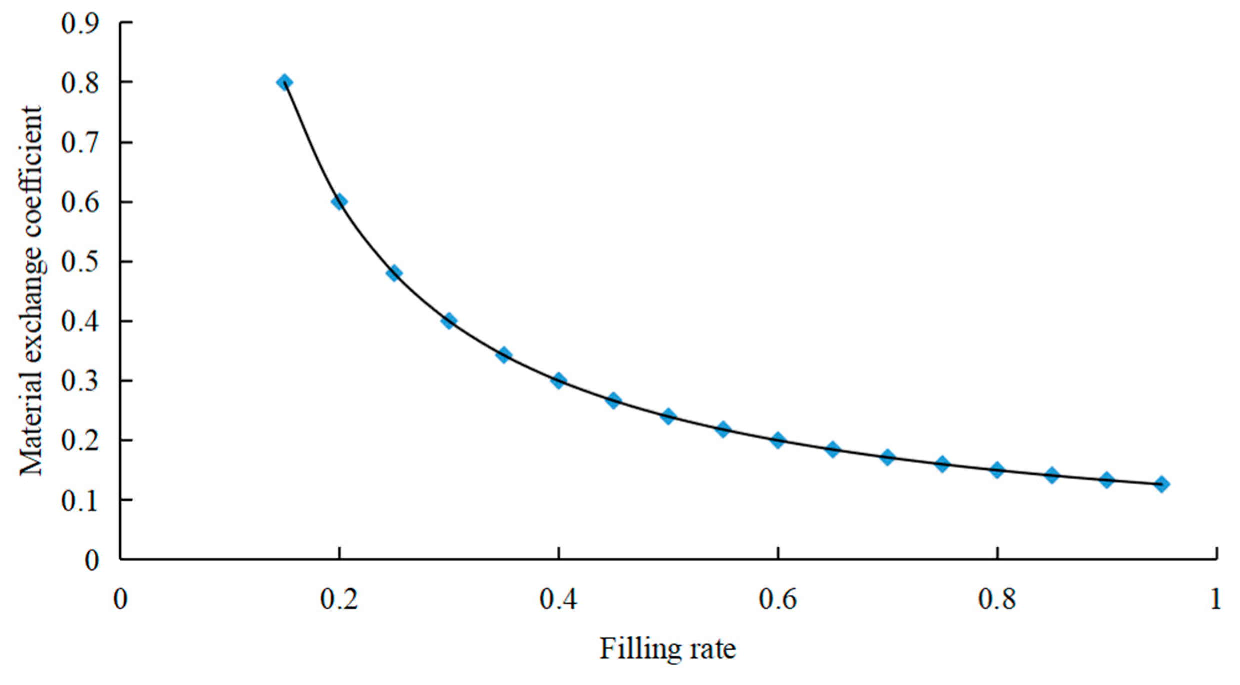
3.2. Model for the Mixing Time

In order to measure the mixing time, which influences the CO₂ emissions during the mixing process, the following models were established according to the structure and mixing mechanism of the mixer. The agitator could be divided into three areas with shaft centers as dividing lines, as shown in Figure 3a, designated as areas I, II, and III. Under the most unfavorable condition, the materials are initially placed on either side of the blade, as shown in Figure 3a, and move from one side to the other during each rotation. The arrows show the direction of material movement as the shafts and blades rotate. Area I is the initial asphalt discharge area, area II is the blade overlap area, and area III is the initial aggregate discharge area. With the increasing number of mixing turns, the materials are uniformly placed in areas I, II, and III, as shown in Figure 3b.

Assume that the asphalt contents of areas I, II, and III are $q_1$, $q_2$, and $q_3$, respectively. During the mixing process, it is assumed that the asphalt content in area II is $q_2=\frac{q_1+q_3}{2}$, which equals the average material mass of areas I and II.

For each rotation circle of the mixing shaft, the exchange coefficient of the material between areas can be calculated using Equation (4).

$$k=\frac{\Delta m}{m}=\frac{\Delta m}{m_0\cdot \eta }=\frac{k_B}{\eta }$$

(4)

where $k$ is the material exchange coefficient at one rotation circle of the mixing shaft; $\Delta m$ is the material exchange mass while the mixing shaft rotates by one cycle, kg; $m$ is the amount of materials in area I, II, or III, kg; $\eta$ is the material filling rate, %; $m_0$ is the mass of materials in area I, II, or III when $\eta =1$, kg; and $k_B$ is the material exchange coefficient at one rotation circle of the mixing shaft when $\eta =1$.

Take areas II and III for analysis. During the mixing process, the amount of asphalt entering area II from area III for each rotation cycle of the mixing shaft can be represented by $\Delta m_3\times q_{3,n}$, and the amount of asphalt entering area III from area II is $\Delta m_2\times q_{2,n}$. After one rotation cycle of the mixing shaft, the asphalt content in area III can be expressed by Equation (5).

$$m\times q_{3,n}=m\times q_{3,(n-1)}-\Delta m_3\times q_{3,(n-1)}+\Delta m_2\times q_{2,(n-1)}$$

(5)

where $m$ is the material mass in area III, kg; $q_{3,n}$ and $q_{2,n}$ are the asphalt content in areas III and II, respectively after the $n_{th}$ ($n\ge 1$) rotation cycle of the mixing shaft, %; $\Delta m_3$ is the material mass that the blades bring from area III to area II while the mixing shaft rotates by one cycle, kg; and $\Delta m_2$ is the material mass that the blades bring from area II to area III while the mixing shaft rotates by one cycle, kg.

Since after one rotation cycle of the mixing shaft the total amount of materials in each area remains unchanged, Equation (6) can be obtained from Equation (4).

$$\Delta m_3=\Delta m_2=k\times m$$

(6)

Substituting Equation (6) into Equation (5) yields Equation (7).

$$q_{3,n}=q_{3,(n-1)}-k\times q_{3,(n-1)}+k\times q_{2,(n-1)}$$

(7)

Using the required asphalt content $q$ to divide Equation (7) then yields Equation (8).

$$\frac{q_{3,n}}{q}=\frac{q_{3,(n-1)}}{q}+k(\frac{q_{2,(n-1)}}{q}-\frac{q_{3,(n-1)}}{q})$$

(8)

Assuming that after $n$ cycles of rotation, the asphalt content in area II is the required asphalt content $q$, then Equation (9) is obtained.

$$\frac{q_{3,n}}{q}=\frac{q_{3,(n-1)}}{q}+k(1-\frac{q_{3,(n-1)}}{q})$$

(9)

When the mixing shaft rotates by $n$ cycles, the relationship between the asphalt content in areas II and III can be expressed by Equation (10). The expressions in square bracket are an infinite series with the first term being “1” and the series ratio being (1 − k). Since 0 < k < 1, when $n\to \infty$ then ${(1-k)}^n\to 0$ and the series converges, and then the sum of $n$ terms is $S_n$, as shown in Equation (11).

$$\frac{q_{3,n}}{q}=\frac{q_{3,0}}{q}+k(1-\frac{q_{3,0}}{q})[1+(1-k)+{(1-k)}^2+{(1-k)}^3+\cdot \cdot \cdot +{(1-k)}^{n-1}]$$

(10)

$$S_n={\frac{1-(1-k)}{k}}^n$$

(11)

During the mixing process, when the deviation of the asphalt content reaches a permissible value, the material is considered to be mixed uniformly (generally, the requirement specifies that the asphalt content deviation should not be greater than 0.3% [32]). Assuming that the mixing number at the desired deviation is $n_0$, $S_n$ can be substituted into Equation (10) to obtain Equation (12).

$$\frac{q_{3,n_0}}{q}=\frac{q_{3,0}}{q}+k(1-\frac{q_{3,0}}{q})\times \frac{1-{(1-k)}^{n_0}}{k}$$

(12)

Considering that at the beginning of mixing, the initial asphalt content in area III is 0, so $q_{3,0}=0$ can be substituted into Equation (12) to obtain Equation (13).

$$n_0=\frac{\log (1-\frac{q_{3,n_0}}{q})}{\log (1-k)}$$

(13)

According to the rotational speed ($N$) of the mixing shaft, the time required for the mixture to be uniformly mixed can be obtained using Equation (14).

$$t_0=\frac{\log (1-\frac{q_{3,n_0}}{q})}{N\log (1-k)}$$

(14)

where $t_0$ is the time required for uniformly mixing the mixture, min; $N$ is the rotational speed of the mixing shaft, min⁻¹.

3.3. Mathematical Model for CO₂ Emissions during Mixing

Substituting Equation (14) into Equations (1) and (2), we can obtain the CO₂ emission calculation model of the mixing process for an engineering project, as shown in Equation (15).

$$E=E_F\cdot \frac{W_1}{W_0}{P}_V{t}_0=\frac{E_F}{60}\cdot \frac{W_1{P}_V\log (1-\frac{q_{3,n_0}}{q})}{W_{0}N\log (1-k)}$$

(15)

where $W_1$ is the total amount of asphalt mixture required for a project, t; $W_0$ is the weight of each pot in the mixer, t.

The method for calculating the power consumption of the mixer ($P_V$) can be obtained from reference [33]. For a mixer with $W_0\ge 1400\mathrm{kg}$, the mixing power ($P_V$) can be calculated according to Equation (16) [33].

$$P_V=30+C{W}_0$$

(16)

where $C$ is the coefficient, kW/kg; for a mixer with $W_0\ge 1400\mathrm{kg}$, $C$ is 0.018 kW/kg [34]. Substituting Equation (16) into Equation (15), we can obtain the CO₂ emission calculation model of the mixing process, as shown in Equation (17).

$$E=\frac{E_F{W}_1(30+0.018W_0)\log (1-\frac{q_{3,n_0}}{q})}{60W_{0}N\log (1-k)}$$

(17)

4. Emission Reduction Analysis and Discussion

Equation (17) reveals that the overall CO₂ emissions ($E$) during the mixing process are proportional to $W_1$, which is the total amount of asphalt mixture required by the project. When $W_1$ is determined, the CO₂ emissions primarily rely on operational parameters $k$ ($k=\frac{k_B}{\eta }$), $\frac{q_{3,n_0}}{q}$, and $W_0$.

Equation (4) shows that as the filling rate $\eta$ increases, the material exchange coefficient $k$ diminishes. Notably, when the value of $\eta$ is small, the $k$ experiences a substantial decrease as the filling rate $\eta$ increases. Conversely, when $\eta$ is relatively large, the decrease in $k$ becomes less pronounced with further increase in $\eta$.

Generally, when a set of blades is installed on the same section of each mixing shaft, the material exchange coefficient $k_B$ is between 0.04 and 0.06; when there are two sets of blades installed on the same cross section, the exchange coefficient is between 0.08 and 0.12. Therefore, according to Equation (4), the relationship between $k$ and $\eta$ in the situation of a set of blades installed on the same cross section can be obtained (as shown in Figure 4). Figure 4 shows that when the filling rate $\eta$ is between 40% and 60%, the change in $k$ from large to small tends to be stable. Consequently, an $\eta$ value of 50% could be considered as a critical threshold. The value of $k$ reaches a stable state when exceeding this point, making it a trade-off between mixing efficiency and energy consumption.

Moreover, according to Figure 4, when $\eta$ is 40%, 50%, and 60%, the corresponding values of $k$ are determined to be 0.2, 0.25, and 0.3, respectively. The relationship curve between the mixing uniformity and the mixing number $n$ is shown in Figure 5 according to Equation (13). The mixing uniformity could be represented by $\frac{q_{3,n_0}}{q}$. A value of $\frac{q_{3,n_0}}{q}$ closes to 1 indicates better mixing uniformity.

Figure 5 represents the relationship between the mixing uniformity and the number of mixing turns. It demonstrates that the enhancement of mixing uniformity exhibits a pattern of rapid improvement followed by a gradual decrease as the mixing number increases. Initially, each increase in the mixing number $n$ results in a significant improvement in mixing uniformity. However, as the mixing number continues to increase, the degree of improvement decreases gradually. Eventually, with further increases in the mixing number, the range of improvement in mixing uniformity becomes minimal. Therefore, it becomes crucial to determine an appropriate mixing number in accordance with the desired requirements of mixing uniformity to prevent excessive mixing numbers, which could lead to unnecessary electricity consumption and an increase in CO₂ emissions.

The above analysis indicates that the requirements for mixing quality have an important impact on the mixing time. Excessive mixing time does not significantly improve the mixing quality, but it does have a substantial impact on CO₂ emissions. Based on Equation (17), assuming the content of asphalt in the mixture is 5%, when the deviation of the asphalt content is 0.2% (the actual content of asphalt is 4.8%), both the mixing time and the CO₂ emission are 1.14 times higher than those observed when the deviation of the asphalt content is 0.3% (the actual content of asphalt is 4.7%). Additionally, if the deviation of the asphalt content is 0.1% (the actual content of asphalt is 4.9%), both the mixing time and the CO₂ emissions are 1.39 times higher than when the deviation is 0.3%, which represents a nearly 40% increase.

Furthermore, Equation (17) highlights the significant influence of the agitator capacity on the CO₂ emissions during mixing, as shown in

Table 2. The agitator capacity and corresponding CO₂ emission reduction.

Number	1	2	3	4	5	6	7	8
Agitator capacity/kg	1500	2000	2500	3000	3500	4000	4500	5000
CO2 emission reduction/%	1	13.2	21.1	26.3	30.1	32.9	35.1	36.8

. For the same engineering quantity, the CO₂ emissions from mixing decrease as the capacity of the agitator increases. Initially, the decrease is substantial, and then the decrease gradually becomes slower. Finally, the decrease becomes stable, as shown in Figure 6. To illustrate the influence of different agitator capacities on CO₂ emissions, comparison analyses were conducted by using agitator types of 2000, 3000, 4000, and 5000 with a reference agitator type of 1500. The results showed that the total CO₂ emissions reduced by 13.2%, 26.3%, 32.9%, and 36.8%, respectively, when using agitators with larger capacities. This implies that for large-scale projects, selecting an agitator with a larger capacity is beneficial for reducing electricity consumption and CO₂ emissions during mixing. In particular, at least the type 4000 agitator is appropriate in this case.

Additionally, the carbon intensity of electricity (which is the amount of CO₂ emitted per unit of electricity generated) is another factor influencing CO₂ emissions during the mixing process. Choosing electricity with a lower-value emission factor can achieve reductions in overall CO₂ emissions. The method used to generate electricity also impacts CO₂ emissions. Since electricity can be generated by using various sources, such as thermal power, hydropower, nuclear power, wind, geothermal, solar power, and so on, it results in different levels of carbon intensity of the electricity. Therefore, reducing the use of carbon-intensive sources of electricity generation and choosing cleaner electricity will significantly lower the CO₂ emissions.

Table 3. Life cycle carbon emission factors for electricity from different generation sources [35].

Electricity Generation Sources	Life Cycle Carbon Emission Factors (kg CO2eq/kWh)
Coal power	1.023
Natural gas	0.434
Solar power	0.037
Wind power	0.012
Hydropower	0.010
Nuclear power	0.005

shows the life cycle carbon emission factors of different electricity generation sources (without carbon capture and storage) [35]. This suggests that the selection of an efficient electricity generation approach could potentially reduce CO₂ emissions by more than 90%.

Overall, according to the above analysis, this paper analyzes the factors influencing CO₂ emissions during the mixing process and proposes measures for emission reduction. The CO₂ emissions generated during the mixing process in a batch asphalt plant exhibit a strong correlation with mixing time. The motor-driven mixer induces material movement in a spiral and cyclic reciprocating motion along the axial direction. After a certain time of mixing, a desired uniform mixture can be achieved. Achieving a uniform mixture involves a trade-off between mixing quality and CO₂ emissions, as the quality inversely correlates with emissions. The mixing time of the mixer is influenced by various factors, including design parameters (such as rotational speed and capacity), operational parameters (such as material filling rate and mixing time), and the quality requirements (mixing uniformity). Once the equipment is employed in the construction site, design parameters are typically fixed, therefore leaving the operational and quality parameters as the primary factors influencing the mixing time. The CO₂ emission model for mixing reveals an initial rapid improvement in mixing quality with increasing time, followed by a gradual decrease until it stabilizes. Therefore, it is necessary to determine an appropriate mixing time based on the mixing quality requirements to avoid excessive mixing time, which does not significantly enhance mixing quality and only leads to heightened electricity consumption and CO₂ emissions. Additionally, the agitator’s capacity is identified as a critical factor impacting emissions. In a given project with a predetermined scope of work, the CO₂ emissions decrease as the agitator’s capacity increases. This highlights the clear advantage of selecting larger capacity agitators, particularly for large-scale projects, to effectively lower electricity consumption and emissions during the mixing process. Furthermore, in alignment with technological advancements, the adoption of cleaner sources of electricity can be an effective strategy for emissions reduction. This holistic approach, considering mixing time optimization, agitator capacity, and cleaner energy sources, presents a multifaceted framework for minimizing CO₂ emissions in asphalt mixture-mixing processes.

5. Conclusions

Through the development of the CO₂ emission calculation model for the mixing process and the exploration of emission reduction technologies, the following conclusions can be drawn:

• The CO₂ emissions model for the mixing process reveals a direct proportional relationship between mixing time and mixing quality, with an initial rapid enhancement followed by gradual improvement and eventual stabilization. It is important to note that an excessive mixing time does not significantly improve the mixing quality but instead significantly escalates electricity consumption and CO₂ emissions.
• For a mixture with 5% asphalt content, when the deviation of the asphalt content is changed from 0.3% to 0.2%, the mixing time and the CO₂ emissions will both increase by 14%. When the deviation is 0.1%, the mixing time and the CO₂ emissions experience a nearly 40% increase.
• The capacity of the agitator also has an important influence on the CO₂ emissions during mixing. Increasing the agitator’s capacity for a given engineering quantity leads to a reduction in overall CO₂ emissions. Initially, this reduction is substantial, followed by a gradually decelerating rate, and it eventually stabilizes. When compared to an agitator of type 1500, employing agitators of types 2000, 3000, 4000, and 5000 yields CO₂ emissions reductions of 13.2%, 26.3%, 32.9%, and 36.8%, respectively. Therefore, for large-scale projects, selecting a high-capacity agitator, preferably of type 4000 or higher, is recommended to minimize electricity consumption and CO₂ emissions during the mixing process.

Overall, this study provides support for optimizing mixture-mixing technology, selecting mixing equipment, and configuring mixing parameters during the road construction process. The findings could contribute to the achievement of emission reduction targets and the promotion of sustainable road development.

References

1. Liu, N.Y.Z.; Wang, Y.Q.; Bai, Q.; Liu, Y.Y.; Wang, P.R.; Xue, S.Q.; Yu, Q.; Li, Q.R. Road life-cycle carbon dioxide emissions and emission reduction technologies: A review. J. Traffic Transp. Eng. Engl. Ed. 2022, 9, 532–555. [Google Scholar] [CrossRef]
2. Stripple, H. Life Cycle Assessment of Road. A Pilot Study for Inventory Analysis. Second Revised Edition; IVL Rapport; IVL Swedish Environmental Research Institute: Gothenburg, Sweden; Linköping, Sweden, 2001. [Google Scholar]
3. Huang, Y.; Bird, R.; Heidrich, O. Development of a life cycle assessment tool for construction and maintenance of asphalt pavements. J. Clean. Prod. 2009, 17, 283–296. [Google Scholar] [CrossRef]
4. Wang, X.; Duan, Z.; Wu, L.; Yang, D. Estimation of carbon dioxide emission in highway construction: A case study in southwest region of China. J. Clean. Prod. 2015, 103, 705–714. [Google Scholar] [CrossRef]
5. Yu, B.; Lu, Q. Estimation of albedo effect in pavement life cycle assessment. J. Clean. Prod. 2014, 64, 306–309. [Google Scholar] [CrossRef]
6. Noland, R.B.; Hanson, C.S. Life-cycle greenhouse gas emissions associated with a highway reconstruction: A New Jersey case study. J. Clean. Prod. 2015, 107, 731–740. [Google Scholar] [CrossRef]
7. Itoya, E.; El-Hamalawi, A.; Ison, S.G.; Frost, M.W.; Hazell, K. Development and Implementation of a Lifecycle Carbon Tool for Highway Maintenance. J. Transp. Eng. 2015, 141, 04014092. [Google Scholar] [CrossRef]
8. Liu, Y.; Wang, Y.; Li, D. Estimation and uncertainty analysis on carbon dioxide emissions from construction phase of real highway projects in China. J. Clean. Prod. 2017, 144, 337–346. [Google Scholar] [CrossRef]
9. Garrain, D.; Lechon, Y. Environmental footprint of a road pavement rehabilitation service in Spain. J. Environ. Manag. 2019, 252, 109646. [Google Scholar] [CrossRef]
10. Blankendaal, T.; Schuur, P.; Voordijk, H. Reducing the environmental impact of concrete and asphalt: A scenario approach. J. Clean. Prod. 2014, 66, 27–36. [Google Scholar] [CrossRef]
11. Tatari, O.; Nazzal, M.; Kucukvar, M. Comparative sustainability assessment of warm-mix asphalts: A thermodynamic based hybrid life cycle analysis. Resour. Conserv. Recycl. 2012, 58, 18–24. [Google Scholar] [CrossRef]
12. Celauro, C.; Corriere, F.; Guerrieri, M.; Lo Casto, B. Environmentally appraising different pavement and construction scenarios: A comparative analysis for a typical local road. Transp. Res. Part D-Transp. Environ. 2015, 34, 41–51. [Google Scholar] [CrossRef]
13. Gulotta, T.M.; Mistretta, M.; Pratico, F.G. A life cycle scenario analysis of different pavement technologies for urban roads. Sci. Total Environ. 2019, 673, 585–593. [Google Scholar] [CrossRef] [PubMed]
14. Santos, J.; Bryce, J.; Flintsch, G.; Ferreira, A.; Diefenderfer, B. A life cycle assessment of in-place recycling and conventional pavement construction and maintenance practices. Struct. Infrastruct. Eng. 2015, 11, 1199–1217. [Google Scholar] [CrossRef]
15. del Carmen Rubio, M.; Moreno, F.; Jose Martinez-Echevarria, M.; Martinez, G.; Miguel Vazquez, J. Comparative analysis of emissions from the manufacture and use of hot and half-warm mix asphalt. J. Clean. Prod. 2013, 41, 1–6. [Google Scholar] [CrossRef]
16. Paranhos, R.S.; Petter, C.O. Multivariate data analysis applied in Hot-Mix asphalt plants. Resour. Conserv. Recycl. 2013, 73, 1–10. [Google Scholar] [CrossRef]
17. dos Santos, M.B.; Candido, J.; Baule, S.D.; de Oliveira, Y.M.M.; Thives, L.P. Greenhouse gas emissions and energy consumption in asphalt plants. Rev. Eletronica Gest. Educ. E Tecnol. Ambient. 2020, 24, e7. [Google Scholar] [CrossRef]
18. Thives, L.P.; Ghisi, E. Asphalt mixtures emission and energy consumption: A review. Renew. Sustain. Energy Rev. 2017, 72, 473–484. [Google Scholar] [CrossRef]
19. Chong, D.; Wang, Y.H.; Chen, L.; Yu, B. Modeling and Validation of Energy Consumption in Asphalt Mixture Production. J. Constr. Eng. Manag. 2016, 142, 04016069. [Google Scholar] [CrossRef]
20. Liu, Y.; Wang, Y.; Lyu, P.; Hu, S.; Yang, L.; Gao, G. Rethinking the carbon dioxide emissions of road sector: Integrating advanced vehicle technologies and construction supply chains mitigation options under decarbonization plans. J. Clean. Prod. 2021, 321, 128769. [Google Scholar] [CrossRef]
21. Aurangzeb, Q.; Al-Qadi, I.L.; Ozer, H.; Yang, R. Hybrid life cycle assessment for asphalt mixtures with high RAP content. Resour. Conserv. Recycl. 2014, 83, 77–86. [Google Scholar] [CrossRef]
22. Saberi, F.K.; Fakhri, M.; Azami, A. Evaluation of warm mix asphalt mixtures containing reclaimed asphalt pavement and crumb rubber. J. Clean. Prod. 2017, 165, 1125–1132. [Google Scholar] [CrossRef]
23. Farina, A.; Zanetti, M.C.; Santagata, E.; Blengini, G.A. Life cycle assessment applied to bituminous mixtures containing recycled materials: Crumb rubber and reclaimed asphalt pavement. Resour. Conserv. Recycl. 2017, 117, 204–212. [Google Scholar] [CrossRef]
24. Rodriguez-Alloza, A.M.; Malik, A.; Lenzen, M.; Gallego, J. Hybrid input-output life cycle assessment of warm mix asphalt mixtures. J. Clean. Prod. 2015, 90, 171–182. [Google Scholar] [CrossRef]
25. Almeida-Costa, A.; Benta, A. Economic and environmental impact study of warm mix asphalt compared to hot mix asphalt. J. Clean. Prod. 2016, 112, 2308–2317. [Google Scholar] [CrossRef]
26. Turk, J.; Pranjic, A.M.; Mladenovic, A.; Cotic, Z.; Jurjavcic, P. Environmental comparison of two alternative road pavement rehabilitation techniques: Cold-in-place-recycling versus traditional reconstruction. J. Clean. Prod. 2016, 121, 45–55. [Google Scholar] [CrossRef]
27. Giani, M.I.; Dotelli, G.; Brandini, N.; Zampori, L. Comparative life cycle assessment of asphalt pavements using reclaimed asphalt, warm mix technology and cold in-place recycling. Resour. Conserv. Recycl. 2015, 104, 224–238. [Google Scholar] [CrossRef]
28. Shi, X. Research on the Mating and Layout of the Equipment and Facilities in the Typical Asphalt Mixture Mixing Plant. Master’s Thesis, Chongqing Jiaotong University, Chongqing, China, 2016. [Google Scholar]
29. IPCC. Climate Change 2014: Mitigation of Climate Change. In Contribution of Working Group III to the Fifth Assessment Report of the Intergovernmental Panel on Climate Change; Cambridge University Press: Cambridge, UK; Cambridge, NY, USA, 2014. [Google Scholar]
30. Roberts, L.; Kandhal, S.; Brown, E.; Lee, D.; Kennedy, T. Hot Mix Asphalt Materials, Mixture Des5ign and Construction, 3rd ed.; NAPA Research and Education Foundation: Lanham, MD, USA, 2009. [Google Scholar]
31. Liu, H.; Liu, N.; Hao, Y.; Zheng, K.; Shao, X. Influence of Mineral Particle Size on Mixing Time and Phase Mixing Technology. China J. Highw. Transp. 2017, 30, 151–158. [Google Scholar]
32. Industrial Standards of the People’s Republic of China. MH/T 5011-2019 Specifications for Asphalt Pavement Construction of Civil Airports; China Civil Aviation Publishing House: Beijing, China, 2019.
33. Wu, Y.; Yao, H. Engineering Machinery Design; China Communications Press: Beijing, China, 2005. [Google Scholar]
34. Liu, H.; Zhou, F.; Wu, S.; Tang, N. Modelling and experimental investigation on mixing technique of graphite modified conductive asphalt mixture. Mater. Res. Innov. 2014, 18, 824–828. [Google Scholar] [CrossRef]
35. UNECE, The United Nations Economic Commission for Europe. Life Cycle Assessment of Electricity Generation Options. 2021. Available online: https://unece.org/sed/documents/2021/10/reports/life-cycle-assessment-electricity-generation-options (accessed on 16 September 2023).
Figure 1. The analysis boundary of the mixing process.
Atmosphere 14 01518 g001
Figure 2. Structure of twin-shaft pugmill agitator: 1 drive motor; 2 mixing cylinder; 3 mixing shaft; 4 mixing blade; 5 synchronizer.
Atmosphere 14 01518 g002
Figure 3. Structure and initial discharge state of the agitator with shaft centers as dividing lines I, II, and III: (a) initial discharge state of the agitator; (b) stable state. The arrows show the direction of material movement as the shafts and blades rotate.
Atmosphere 14 01518 g003
Figure 4. Correlation between material exchange coefficient ( k ) and filling rate (η).
Atmosphere 14 01518 g004
Figure 5. Correlation between mixing uniformity and mixing number.
Atmosphere 14 01518 g005
Figure 6. The curve of agitator capacity and corresponding CO2 emission reduction.
Atmosphere 14 01518 g006