On the Impact of ENSO Cycles and Climate Change on Telescope Sites in Northern Chile

Abstract

The Atacama desert stands as the most arid, non-polar, region on Earth and has accommodated a considerable portion of the world’s ground-based astronomical observatories for an extended period. The comprehension of factors important for observational conditions in this region, and the potential alterations induced by the escalating impact of climate change, are, therefore, of the utmost significance. In this study, we conduct an analysis of the surface-level air temperature, water vapour density, and astronomical seeing at the European Southern Observatory (commonly known by its acronym, ESO) telescope sites in northern Chile. Our findings reveal a discernible rise in temperature across all sites during the last decade. Moreover, we establish a correlation between the air temperature and water vapour density with the El Niño Southern Oscillation (ENSO) phases, wherein, the warm anomaly known as El Niño (EN) corresponds to drier observing conditions, coupled with higher maximum daily temperatures favouring more challenging near-infrared observations. The outcomes of this investigation have potential implications for the enhancement of the long-term scheduling of observations at telescope sites in northern Chile, thereby aiding in better planning and allocation of resources for the astronomy community.

1. Introduction

The Atacama climate is primarily influenced by large-scale subsidence at subtropical latitudes. However, the combination of the Andean slope and the adjacent cold Humboldt stream in the Pacific Ocean also makes a significant contribution [1]. This interaction results in an atmospheric marine boundary layer characterised by extremely dry and cloud-free air above it (relative humidity below $15\%$), providing favourable conditions for astronomical observations [2].

It is precisely this fortuitous geography, with extremely dry and cloud-free air at high altitudes that makes the Atacama desert the primary host of world-class astronomical facilities in the world. Not only does northern Chile already host the vast majority of 8 m class visible and near-infrared telescopes, but it is also the construction site of the world’s first 40 m class telescope, the Extremely Large Telescope (ELT). Important factors for the data quality in cutting-edge astronomy are the integrated absolute humidity (precipitable water vapour, PWV), together with meteorological conditions, such as the surface air temperature, wind speed, and relative humidity [3,4]. PWV and its proxy, the surface water vapour density (WVD), are relevant in the near- to mid-infrared range, as water vapour affects the astronomical observations via atmospheric absorption and thermal emissions [5,6]. This means the absorption of light by the water in Earth’s atmosphere significantly reduces the light received by telescopes, especially in the near-infrared. Observing schedules at the European Southern Observatory, the focal point of this work, are created up to half a year in advance when weather conditions are still unclear. Therefore, if too many observational programmes with strong constraints on precipitable water vapour are scheduled, but then atmospheric conditions do not allow for them, the telescopes will end up with fewer observable programmes in the scheduling period than were needed. In other words, during observing nights with adequate but not excellent observing conditions, where less restrictive observations could have been observed, the telescopes are needlessly sitting idle. This lost time is aptly called idle time and should be avoided as much as possible. To this date, the astronomy community has no metric on which to base the average conditions beyond the known annual seasonal variations, and the impact of climate change on the future of infrared programmes is uncertain at best.

In addition to the scheduling issue, the overall quality of observations during a specific night is an important metric to assess the suitability of an observing site. In the visible and near-infrared, astronomers employ the seeing term for this purpose. In simple terms, seeing is a measure of the angular broadening of an astronomical point-like source on the image plane due to Earth’s atmospheric turbulence. It is expressed in arcseconds, a unit of small angles common in astronomy, where one arcsecond is equal to $\frac{1}{3600}$ of a sexagesimal degree. The smaller the seeing magnitude the better resolved the image of the observed object. Excellent seeing for astronomical research is defined as seeing below 0.6${}^{″}$ and indicates a near-motionless image. Median level seeings range from 0.6${}^{″}$ to 0.9${}^{″}$. Acceptable seeing ranges from 1.5${}^{″}$ up to 2.0${}^{″}$ at which levels the image starts to become more distorted. Important factors affecting the turbulent mixing of the atmospheric layers, and hence affecting the seeing, are the vertical gradients of the horizontal wind speed and temperature gradients [7], and references therein. It remains a topic of much interest to know whether astronomical seeing is affected by long-term climate oscillations or climate change, a point to which we aim to contribute in this manuscript. In the context of the long timescale and associated cost for the construction and the subsequent operation of the ELT in the next half century, an assessment and hopefully a predictive tool of overall atmospheric conditions and seeing is crucial for the community.

In this work, we aim to fill this knowledge gap for the astronomy community by assessing the suitability of ENSO as a predictive tool for interannual condition changes. The prominent feature of the El Niño (EN) phase of ENSO is the warming of the tropical Pacific, quantified by the Niño3.4 index, leading to increased near-surface air temperatures down to 30${}^{\circ }$ S—encompassing all observatories in this study along the Pacific coast of South America. Its counterpart, La Niña (LN), is marked by opposite conditions. While EN phases have been correlated with higher precipitation in the 30${}^{\circ }$–41${}^{\circ }$ S latitudes band [8], the subtropical region, where the Atacama Desert lies, has been correlated with dryer conditions [9].

Hence, we assess the impact of ENSO phases and global warming trends on WVD and temperature for European Southern Observatory sites, providing essential metrics for the community to evaluate long-term observational conditions in northern Chile. We propose strong ENSO phases as a metric to better schedule challenging observing programmes, but find no significant impact of global warming on astronomical site quality. However, we confirm the globally seen warming trend and explore local effects on high altitude sites and curious local cooling effects impacting the Paranal Observatory specifically. With regards to seeing, we show that the median seeing conditions remain stable within the natural inter-annual variability, a crucial result in the context of the ELT. The manuscript is structured as follows: In Section 2, we provide an overview of the sites, the acquired data, and the analysis methods. In Section 3, we link the data to climate indices and explore the connection to climate change. We then provide important conclusions for the astronomy community in Section 4 where we highlight the power of established climate indices to prevent time loss due to sub-optimal planning and provide an outlook for future studies to monitor seeing in a warming climate.

2. Materials and Methods

2.1. Data Collection and Accessibility

For this study, we collected data from three different observatories at four different sites (see overview in

Table 1. Location of all European Southern Observatory sites used for data collection in this study.

Observatory	Latitude [${}^{\circ }$S]	Longitude [${}^{\circ }$W]	Elevation [MASL]
la Silla	29.258	70.738	2400
Paranal	24.627	70.404	2650
Llano del Chajnantor (CBI)	23.0333	67.7667	5080
Llano del Chajnantor (APEX)	23.0058	67.7592	5150

). We provide instructions on how to access all the data in this study in the Data Availability Statement at the end of the manuscript. An overview of the coverage and further details are presented in

Table 2. Data provided from the respective meteo station (T and RH at 2 m).

Site	Obs Period	Time Resolution	#Days with Obs	% of Coverage
la Silla	10-May to 23-April	1 min	4740	$91.20\%$
Paranal	98-July to 23-April	1 min	13,997 1	$91.86\%$1
	84-November to 98-June	20 min to h +	-	-
CBI	99-April to 5-July	1 h	2867	$77.01\%$
APEX	6-January to 23-April	1 min	6050	$98.61\%$

¹ Combining historical and current data.

.

2.1.1. La Silla

The Astronomical Weather Station (AWS) started routine operation in September 1991 and full automation was reached in December 1993. From October 1988 to February 1991, measurements were conducted from Cerro Vizcachas, 7 km to the east of La Silla, which was once a candidate site for the Very Large Telescope (VLT). In 2008, the AWS was struck by lightning and had to be replaced by a new weather station and sensors. This replacement was completed in May 2010. However, the data before this event show a marked offset in pressure, jumping from previously approximately 774 hPa median pressure to 769 hPa median pressure. This change is also visible in different temperatures and dew points before and after the event. It is unclear whether this difference is due to a change in the location of the AWS (no such change was recorded) or if the values were previously recorded at 30 m and then at 2 m, but saved in the database as a continuous series at 2 m. Due to this inconsistency, we focus our study on the data after the lightning strike, with the new AWS station (2010 and beyond).

2.1.2. Paranal Observatory

The temperature at different altitudes for the Paranal Observatory, as well as the relative humidity and the wind direction, were obtained from the European Southern Observatory ambient query form. However, the ambient query form only contains data from the Vaisala Meteorological station at the Paranal Observatory since August 1998 when the station was upgraded. We obtained the historical values since its installation in October 1984 from European Southern Observatory internal documents. Measurements were suspended from July 1991 to September 1992 for the 14-month duration of the levelling work of the Paranal Observatory peak to make the platform needed to install the VLT. No offsets were found in the data due to this intervention. Values are sparse in the historical data until April 1994 (one or two daily measurements) and then show a 20-minute cadence. The sparse data are not taken into account in our analysis but are available upon request. No change points were found between the historical data and the current data.

The optical turbulence at the Paranal Observatory is measured with the help of two instruments that share the same optical tube assembly. The integrated turbulence along the atmospheric column is measured with a differential image motion monitor (DIMM) instrument [10]. Sharing the field-of-view is the multi-aperture scintillation sensor (MASS) instrument [11], which provides a measure of the vertical profile of the optical turbulence. The MASS helps to obtain the integrated seeing in the troposphere, 250m above the surface level and beyond. Hence, these instruments have proven important to monitor both the integrated turbulence in the whole atmosphere above the DIMM level (currently 7 m above the surface) and the seeing in the free-troposphere.

2.2. Paranal Observatory Precipitable Water Vapour and Water Vapour Density Calculation

The PWV measurements from the Paranal Observatory were obtained via two sources. Starting from April 2015, PWV measurements were performed with the LHATPRO (Low Humidity And Temperature PROfiling, [12]) instrument. This is a microwave radiometer covering the strong water vapour emission line at 183 GHz, and providing a record of measurements with a time resolution of a few seconds. Historical values are available at a lower time sampling from the observation of the equivalent width telluric standard stars under clear sky conditions with the XSHOOTER and UVES instruments. PWV measurements from XSHOOTER, at an average sampling rate of every three hours, are available from October-2009 to March-2020, while one daily measurement or less from UVES is available from April-2000 to September-2020. The data, as monthly median values for the Paranal Observatory, are shown in Figure 1; no augmentation in minimum PWV with time is discernible. When data from more than one measurement were available, we verified that the difference between the data was less than $1\sigma$ and then provided the mean in the plot. No conflicting data points were found and the measurements from XSHOOTER and UVES confirmed the new LHATPRO measurements. The PWV of the Chajnantor site has been studied in detail in [13]. Unfortunately, for the la Silla Observatory, no such observations exist. Given that we are mainly interested in the impact on surface conditions at telescope sites, we use the water vapour density (WVD) as a proxy for all three sites.

The water vapour density (WVD) is calculated from the relative humidity (RH) and the temperature (T) at the altitude of the meteorological sensors station. The water vapour pressure at saturation $e_{\mathrm{sat}}$ is derived from these two parameters via the solution of the Clausius–Clapeyron equation from [14]:

$$e_{\mathrm{sat}}=6.1121·exp\frac{17.502T_c}{240.97+T_c}·100\left[\mathrm{Pa}\right]$$

(1)

where $T_c$ is the temperature in degrees Celsius. The nominal water vapour pressure is then

$$e_0=e_{\mathrm{sat}}·\frac{\mathrm{RH}}{100}\left[\mathrm{Pa}\right]$$

(2)

and, following the ideal gas law,

$$\mathrm{WVD}=\frac{e_0}{R_v{T}_K}·1000\left[\frac{\mathrm{g}}{{\mathrm{m}}^3}\right]$$

(3)

with $T_K$ the temperature in Kelvin, and $R_v$ as the specific gas constant for water vapour ($461.5\frac{J}{\mathrm{K}·\mathrm{kg}}$), the WVD can be derived for all three observatory sites.

2.3. Paranal Observatory Turbulence Quantification

We use the computed surface level temperature and wind speed gradients to produce an overall estimate of the Richardson number as a proxy for turbulence. The Richardson number is the result of taking the ratio between the buoyancy forces and the square of the wind shear, and is computed as follows:

$$\mathcal{R}i=\frac{g}{\theta }\frac{\frac{d\theta }{dh}}{{\left(\frac{dU}{dh}\right)}^2}\left[\mathrm{adimentional}\right]$$

(4)

$$\theta =T\left[\mathrm{K}\right]{\left(\frac{P_0}{P}\right)}^{R/c_p}\left[\mathrm{K}\right]$$

(5)

where g is the acceleration of gravity (9.8 $\frac{\mathrm{m}}{{\mathrm{s}}^2}$), $\theta$ is the mean air potential temperature, $d\theta /dh$ is the vertical gradient of air potential temperature, and $dU/dh$ is the vertical gradient of the horizontal wind speed. $P_0$ is the pressure at a reference altitude level (the sea level, ∼1013 hPa), R is the gas constant of mixed air ($287.05$ $\frac{\mathrm{J}}{\mathrm{K}·\mathrm{kg}}$), and $c_p$ is the specific heat capacity at constant pressure ($1005.0$ $\frac{\mathrm{J}}{\mathrm{K}·\mathrm{kg}}$).

2.4. Missing Values and Consistency

Some of the historical data show sections of missing data, some as large as years, but mostly one value or two during the day. In the cases where only one value was missing consecutively, we applied a linear interpolation before building monthly sums or means. In cases where more than one value was missing in a row, the missing value was treated like a propagating NaN. For consistency, we checked that the maximum daily value was not below the minimum daily value of the previous day [15]. No inconsistent values were found. In order to avoid an undue influence of outliers on our analysis of the minimum and maximum values, we calculate extremes as the $0.5\%$ and $99.5\%$ percentile values, respectively.

2.5. Trends and Correlation Calculation

The seasonal trends were calculated for the austral seasons: summer (December to February, DJF), autumn (March to May, MAM), winter (June to August, JJA), and spring (September to November, SON). The summer season thus commences in the December of the previous calendar year. As we are principally interested in the impact on astronomical sites, the data were separated into day and night by calculating the time when the sun zenith angle was ${90}^{\circ }$ at the telescope site (i.e., above the horizon). Considering that temperatures usually follow non-normal distributions, we applied the non-parametric Mann–Kendall test to estimate trends [16] with the removal of potential auto-correlation in time series [17], as implemented in [18]. In this implementation, trends are established with a Kendall’s $\tau$-based slope estimator [19], with statistical significance set to the $5\%$ level (p-value). We estimated the correlation between our observed parameters and modes of climate variability with a Student’s t-test. The resulting Pearson’s correlation coefficient (PCC) is shown, together with the p-value. The significance level of the correlation is set at $5\%$ (p-value).

2.6. Climate Indices

The general atmospheric circulation can be disturbed by internal modes—large-scale disruptions due to the unstable coupling of the atmosphere–ocean system. This cyclical climate variability plays an important role in South America’s climate on both sides of the Andean Cordillera, as recently highlighted in [20], where changes in the surface wind of western Patagonia were linked to ENSO and PDO modes. The three most important large-scale modes of climate variability in South America are described as the Antarctic circulation (AAO, [21]), and the aforementioned long-term Pacific decadal oscillation (PDO, [22]) and El Niño-Southern Oscillation (ENSO, [23]). In this work, we will mostly focus on ENSO and provide only a surface definition of the other two phenomena and their impact.

The AAO is the main component of the 850 hPa geopotential height anomalies south of ${20}^{\circ }$S but also influences temperature and precipitation anomalies in South America, e.g., the AAO is associated with precipitation anomalies in southern Chile and the subtropical east coast of the continent [24]. The PDO is the main reason for the monthly sea surface temperature anomalies in the Pacific Ocean (north of 20${}^{\circ }$ N) with a decadal oscillation between warm and cold phases. The ENSO operates on shorter cycles ranging between 2 and 7 years and is typically separated into two anomaly cycles: El Niño (EN, warm phase) and La Niña (LN, cold phase), where occurrences in the EN phases are usually roughly inverse to the LN phases. The ENSO is monitored via various indices with the Niño3.4 index the most appropriate choice for northern Chile [25]. Niño3.4 quantifies the SST anomaly between 5${}^{\circ }$ N–5${}^{\circ }$ S and between 170–120${}^{\circ }$ W and was obtained from the National Oceanic and Atmospheric Administration of the U.S. Department of Commerce as a monthly mean time series. An EN or LN phase is declared when the temperature anomaly deviates $>|0.5{}^{\circ }\mathrm{C}|$ from the historical mean. We define strong LN or EN phases by a deviation of $>|0.75{}^{\circ }\mathrm{C}|$ from the historical mean.

3. Results

3.1. European Southern Observatory Sites Temperature Trends

All sites in our study are found at geographical elevations 2400 m above sea level (MASL). However, both the la Silla and the Paranal Observatory are close to the coastal line and at the lower boundary of high-elevation sites. On the other hand, the Chajnantor site lies at over 5000 MASL on the western slope of the Andes mountains. This allows us to provide some insights into how temperature trends change with altitude. The significance of temperature trends, as a function of site (altitude), was assessed using the Mann–Kendall (MK) test. See Appendix A for the tables for all sites together with a more in-depth analysis of the temporal warming variations for the Paranal Observatory (Appendix A-

Table A2. Temperature trends Paranal Observatory, 1994–2009.

Season		Trend	p-Value	$\mathit{\tau }$	Slope
DJF (day)	mean	no trend	$0.111$	-	-
	max	increasing	$0.004$	$0.361$	$0.110$
	min	decreasing	$0.013$	$-0.190$	$-0.030$
DJF (night)	mean	no trend	$0.515$	-	-
	max	increasing	$0.012$	$0.257$	$0.091$
	min	decreasing	$0.000$	$-0.324$	$-0.083$
MAM (day)	mean	no trend	$0.135$	-	-
	max	decreasing	$0.000$	$-0.253$	$-0.095$
	min	increasing	$0.003$	$0.198$	$0.078$
MAM (night)	mean	no trend	$0.676$	-	-
	max	decreasing	$0.029$	$-0.187$	$-0.070$
	min	no trend	$0.222$	-	-
JJA (day)	mean	no trend	$0.496$	-	-
	max	no trend	$0.162$	-	-
	min	no trend	$0.205$	-	-
JJA (night)	mean	no trend	$0.062$	-	-
	max	no trend	$0.122$	-	-
	min	increasing	$0.010$	$0.282$	$0.196$
SON (day)	mean	no trend	$0.205$	-	-
	max	no trend	$0.565$	-	-
	min	no trend	$0.403$	-	-
SON (night)	mean	no trend	$0.614$	-	-
	max	no trend	$0.428$	-	-
	min	no trend	$0.168$	-	-

and

Table A3. Temperature trends Paranal Observatory, 2010–2023.

Season		Trend	p-Value	$\mathit{\tau }$	Slope
DJF (day)	mean	no trend	$0.111$	-	-
	max	increasing	$0.004$	$0.362$	$0.110$
	min	no trend	$0.261$	-	-
DJF (night)	mean	no trend	$0.515$	-	-
	max	increasing	$0.012$	$0.257$	$0.091$
	min	no trend	$0.102$	-	-
MAM (day)	mean	no trend	$0.135$	-	-
	max	decreasing	$0.001$	$-0.187$	$-0.095$
	min	increasing	$0.003$	$0.231$	$0.078$
MAM (night)	mean	no trend	$0.676$	-	-
	max	decreasing	$0.029$	$-0.187$	$-0.054$
	min	increasing	$0.002$	$0.253$	$0.230$
JJA (day)	mean	no trend	$0.917$	-	-
	max	no trend	$0.162$	-	-
	min	no trend	$0.205$	-	-
JJA (night)	mean	no trend	$0.918$	-	-
	max	no trend	$0.702$	-	-
	min	increasing	$0.010$	$0.282$	$0.196$
SON (day)	mean	no trend	$0.609$	-	-
	max	no trend	$0.410$	-	-
	min	no trend	$0.089$	-	-
SON (night)	mean	no trend	$0.714$	-	-
	max	no trend	$0.168$	-	-
	min	no trend	$0.212$	-	-

).

Our results show a significant increase in temperatures at the Chajnantor site, with rising trends for temperatures during the austral summer. These trends confirm the projected altitude-dependent warming acceleration, both globally [26] and for future observatories [27]. In the austral autumn, the minimum temperatures at the Chajnantor site exhibit an increase of $1{}^{\circ }\mathrm{C}/$decade, twice as fast as any other parameter. A consistent rise in the minimum temperature during the austral autumn (and the maximum temperature in summer) extends across all sites. Previous studies on climate trends in Chile have demonstrated substantial warming during the austral autumn and summer while suggesting cooling during spring and winter [28] linked to climate change [29]. Our findings corroborate a strong warming trend, specifically evident in the minimum temperature during autumn, which implies reduced cool periods leading up to winter. This indicates a lengthening of the ablation season in the high Andes with an impact on the glacier mass balance [28]. Nonetheless, the climate forcing responsible for glacial shrinkage in Chile is a complex subject [30] and beyond the scope of this work.

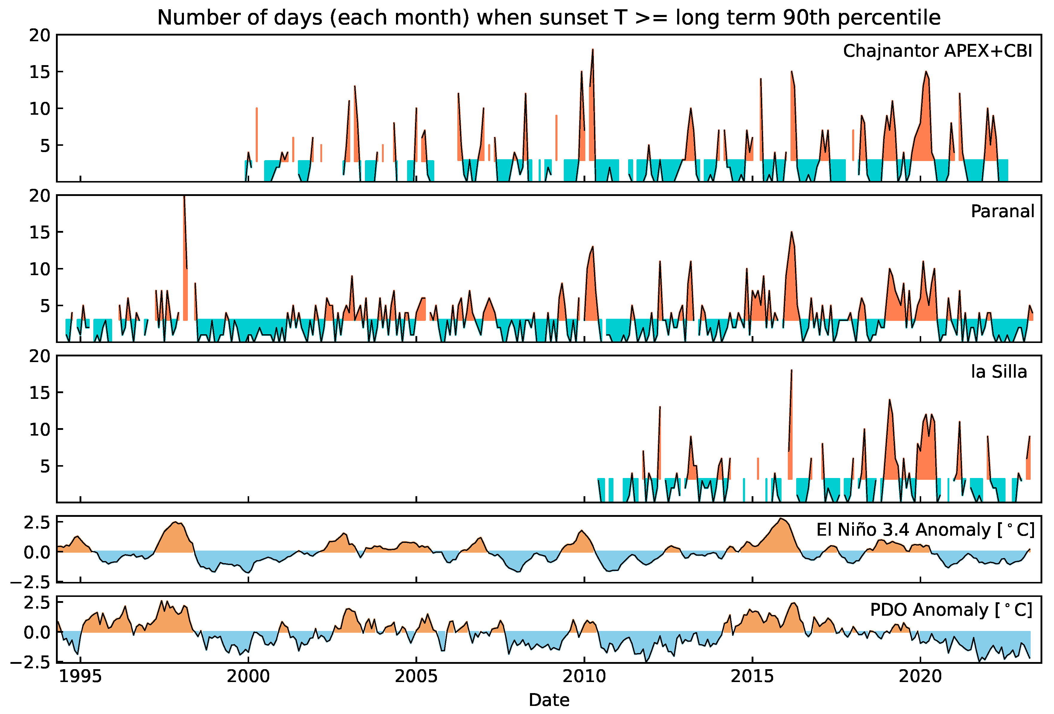
While a definitive warming trend attributed to global warming is evident across European Southern Observatory sites, annual-level variations cannot be solely ascribed to climate change. We investigated the link between extreme warm events when the daily maximum ambient temperature exceeded the 90th percentile of the long-term temperature record and ENSO (Figure 2). Our findings reveal a distinct correlation between the occurrence of warm surface temperature anomalies and the Niño3.4 index across sites. Further details on the correlations for all sites can be found in

Table 3. Student’s t-test for correlation between El Niño3.4 anomaly and sunset temperature outliers (see Figure 2).

Observatory	PCC	p-Value
Chajnantor (CBI+APEX)	$0.192$	$0.004$	correlation
Paranal	$0.453$	$0.000$	correlation
la Silla	$0.228$	$0.012$	correlation

and in Appendix A.

3.2. European Southern Observatory Sites Surface Water Vapour Density Trends and Precipitable Water Vapour

The surface water vapour density (WVD) in the Paranal and the la Silla Observatories is anti-correlated with ENSO (see

Table 4. Student’s t-test for correlation between el Niño3.4 anomaly annual maximum value of WVD monthly medians.

Observatory	PCC	p-Value
Chajnantor (APEX)	-	$0.385$	no correlation
Paranal	$0.134$	$0.022$	anti-correlation
la Silla	$0.380$	$0.000$	anti-correlation

). Years during strong EN phases show no surface-level wet periods, while there are a larger number of days with temperatures above the long-term 90th quantile, e.g., in 1998, in 2010, and in 2016 (see Figure 3). While a decrease in WVD is also observed for the Chajnantor site during strong EN phases, the overall WVD is extremely low, and no correlation could be determined in our short data series. The most important site to quantify is the Paranal Observatory due to its close proximity to the construction site (Cerro Armazones) of the future Extremely Large Telescope (ELT) [31].

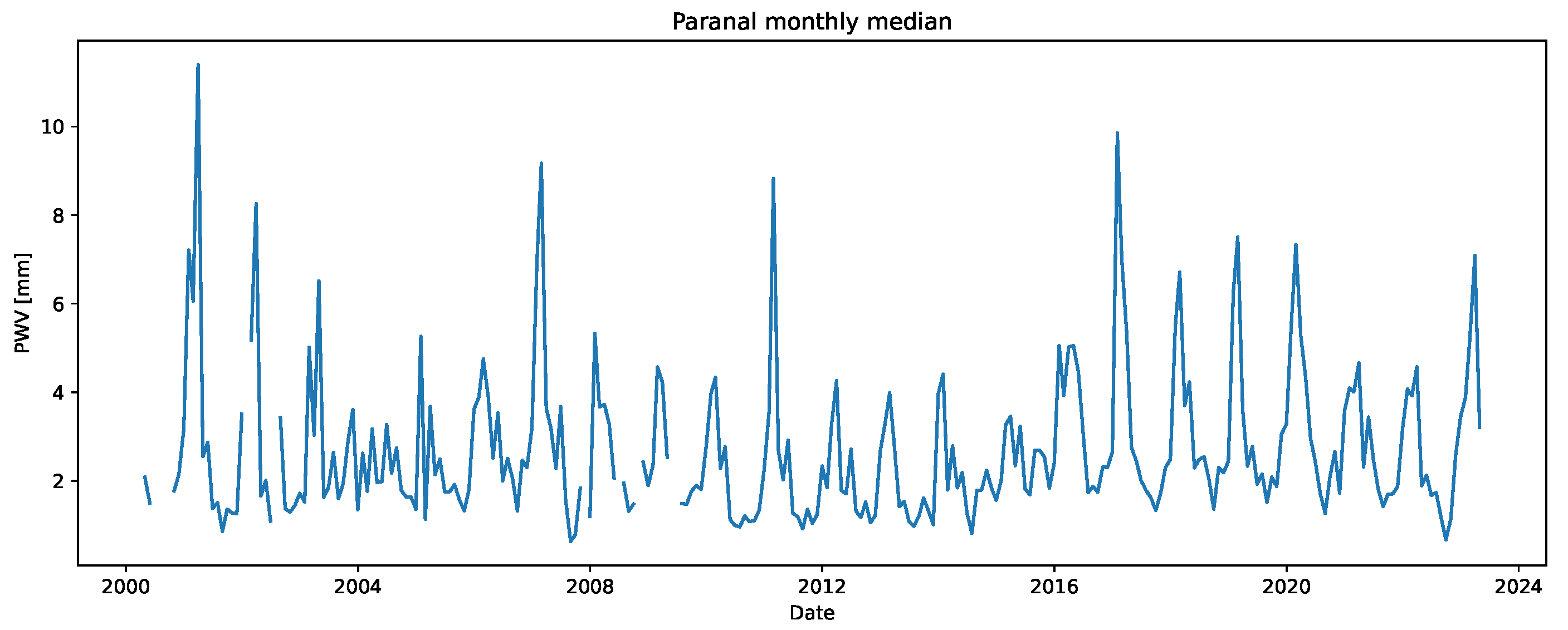
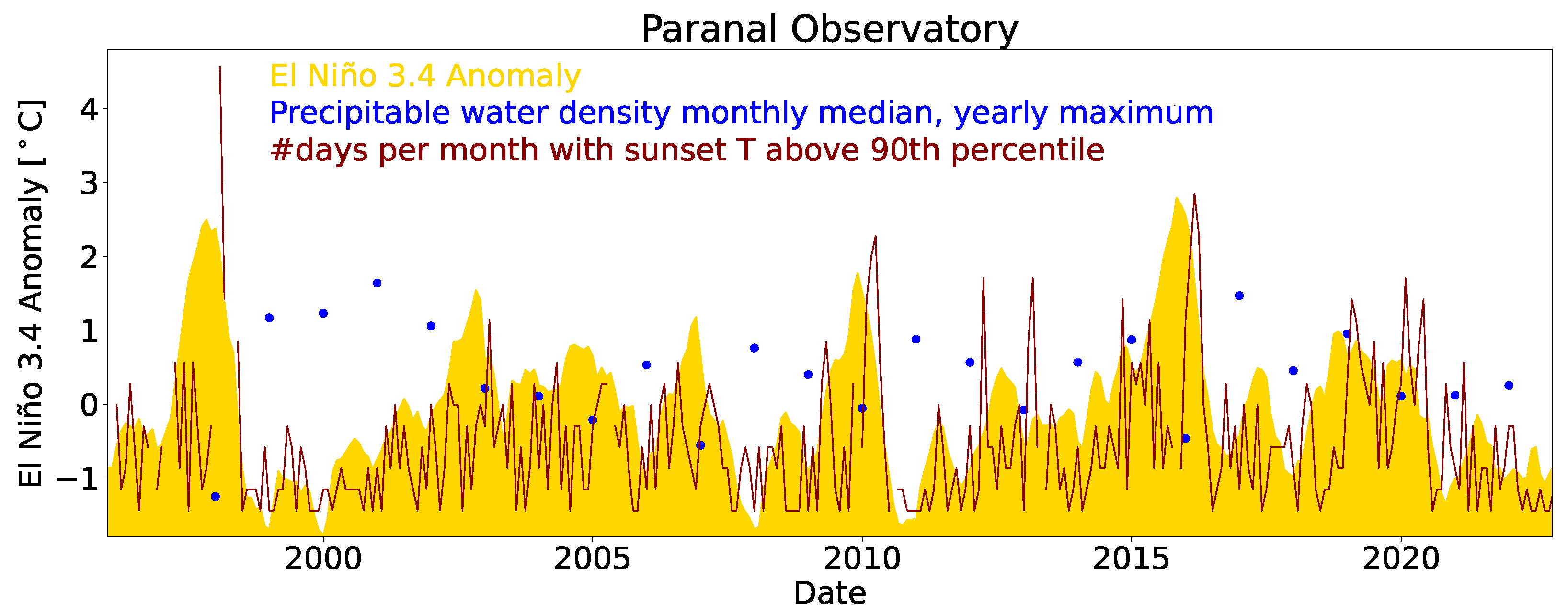
The monthly median values of precipitable water vapour (PWV) for the Paranal Observatory are shown in Figure 1 and no augmentation in minimum PWV with time is discernible; however, a marginal decadal oscillation can be inferred. If anything, what is clearly visible is the variability in the maximum PWV events during the austral summers. This variability is most likely influenced by the predominant position of the Bolivian high-pressure centre during summer months [32,33,34], which leads to dry anomalies during the normally wet summer for the combination of EN/PDO(+) [9]. The PWV long-term record for the Chajnantor site was analysed in [13], and no evidence of PWV trends over the 20 years of data was found, in agreement with our results for the Paranal Observatory.

3.3. The Impact on Astronomical Seeing

In observational astronomy, and as a more technical addition to the definition in Section 1, seeing is a term that refers to the broadening in the point-spread-function (PSF) of a point-like source (a star) attributed to atmospheric optical turbulence. The broadening occurs due to the scattering of light away from the core of the PSF because of rapid fluctuations in the air index of refraction along the path the starlight follows through the atmosphere to an imaging detector.

In optical wavelengths, the index of refraction fluctuation is dominated by the turbulent mixing of air of different temperatures [35]. The effects of turbulent fluctuations of humidity in the air index of refraction are more relevant for light in the infrared and radio wavelengths [36]. In this paper, we refer to seeing, in the optical band, more specifically as measured by the differential image motion monitor (DIMM) instrument at a wavelength of 500 nm. In simple terms, seeing is a measure of the angular size, in arcsecs, of the PSF at the half-intensity point and at the first order driven by changes in wind direction and temperature gradients. While it is understood in detail how seeing is influenced by environmental parameters, predictive tools for seeing on longer time scales are not available to the community.

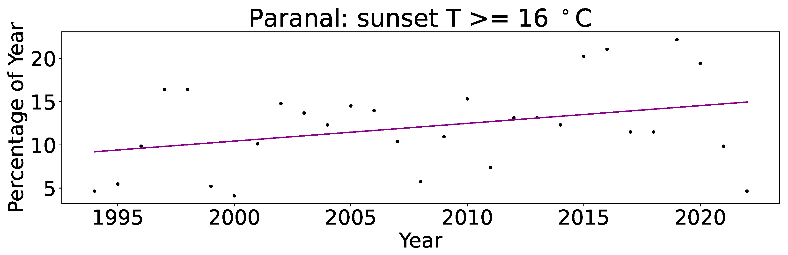
In the context of the ELT, the impact of climate variations on atmospheric turbulence and, thus, seeing at the Paranal Observatory is of the utmost importance. As stated above, the temperature gradient has an important impact on seeing. This gradient is naturally largest at sunset when the surface and telescope domes are heated from the strong solar irradiation in the Atacama desert. The authors of [37] studied the amount of time each year that the sunset temperature was above 16 ${}^{\circ }$C for the period 2008–2020. The value of 16 ${}^{\circ }$C is the maximum temperature at which the telescope dome environments can be maintained while still providing safe cooling to the electronics equipment. We have expanded the analysis to include the full available time series 1994 to 2022 and confirm their trends (see Figure 4). The yearly fraction of sunset surface air temperatures exceeding 16 ${}^{\circ }$C has increased at a rate of over $2\%$ per decade, reaching up to a 20–25% yearly fraction during the last EN phase in 2018–2019. This trend is in line with global warming, as confirmed via the MK statistical test. Because of the necessary cooling within the telescope dome environments, on warmer days (temperatures at sunset above 16 ${}^{\circ }$C), the domes are cooler than the external ambient temperature at the time of dome opening. 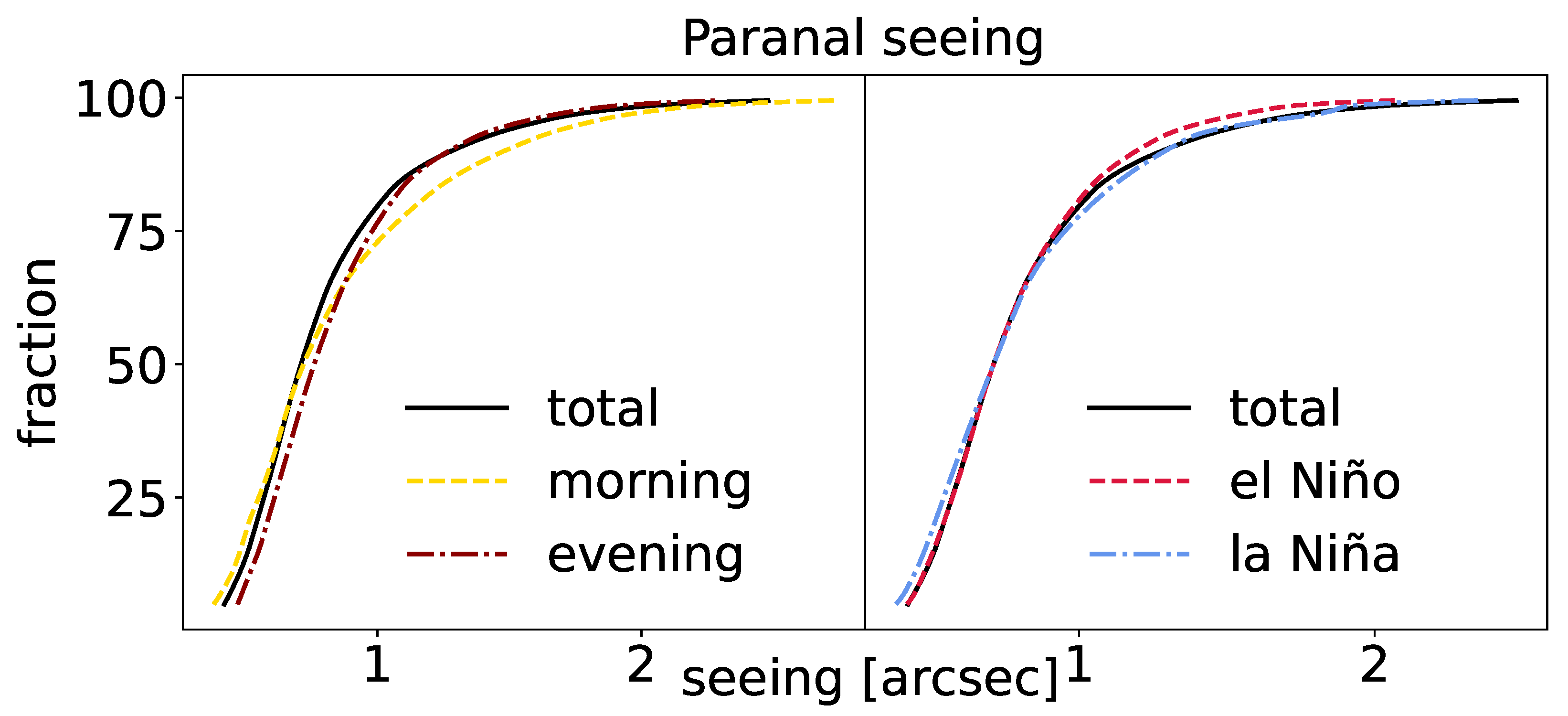In [37], it is inferred that this particular temperature gradient leads to stronger turbulence. However, we may argue that the internal and cooler atmosphere inside the dome is stratified and convection is, thus, inhibited. That said, this may require a specific study on the science image quality as a function of the difference in temperature between the internal dome environment and the external air. At least, in terms of atmospheric seeing, our study of evening and morning twilight seeing compared to total seeing for the most affected years (2016–2021) shows that the fraction of high-seeing events (>1.6 arcseconds) for the evening twilight is equal to the total seeing statistics (see Figure 5 and

Table A5. Probability density function of mean seeing during the period 2016 to 2021.

Fraction	Total Nights	Morning Twilight	Evening Twilight
$5\%$	$0.42$	$0.38$	$0.47$
$10\%$	$0.47$	$0.44$	$0.51$
$15\%$	$0.51$	$0.48$	$0.55$
$20\%$	$0.54$	$0.51$	$0.58$
$25\%$	$0.57$	$0.55$	$0.61$
$50\%$	$0.71$	$0.72$	$0.76$
$75\%$	$0.93$	$1.04$	$0.98$
$90\%$	$1.28$	$1.48$	$1.27$
$95\%$	$1.57$	$1.77$	$1.51$
$97.5\%$	$1.84$	$2.04$	$1.75$
$99\%$	$2.22$	$2.43$	$2.06$
$99.5\%$	$2.48$	$2.73$	$2.3$

).

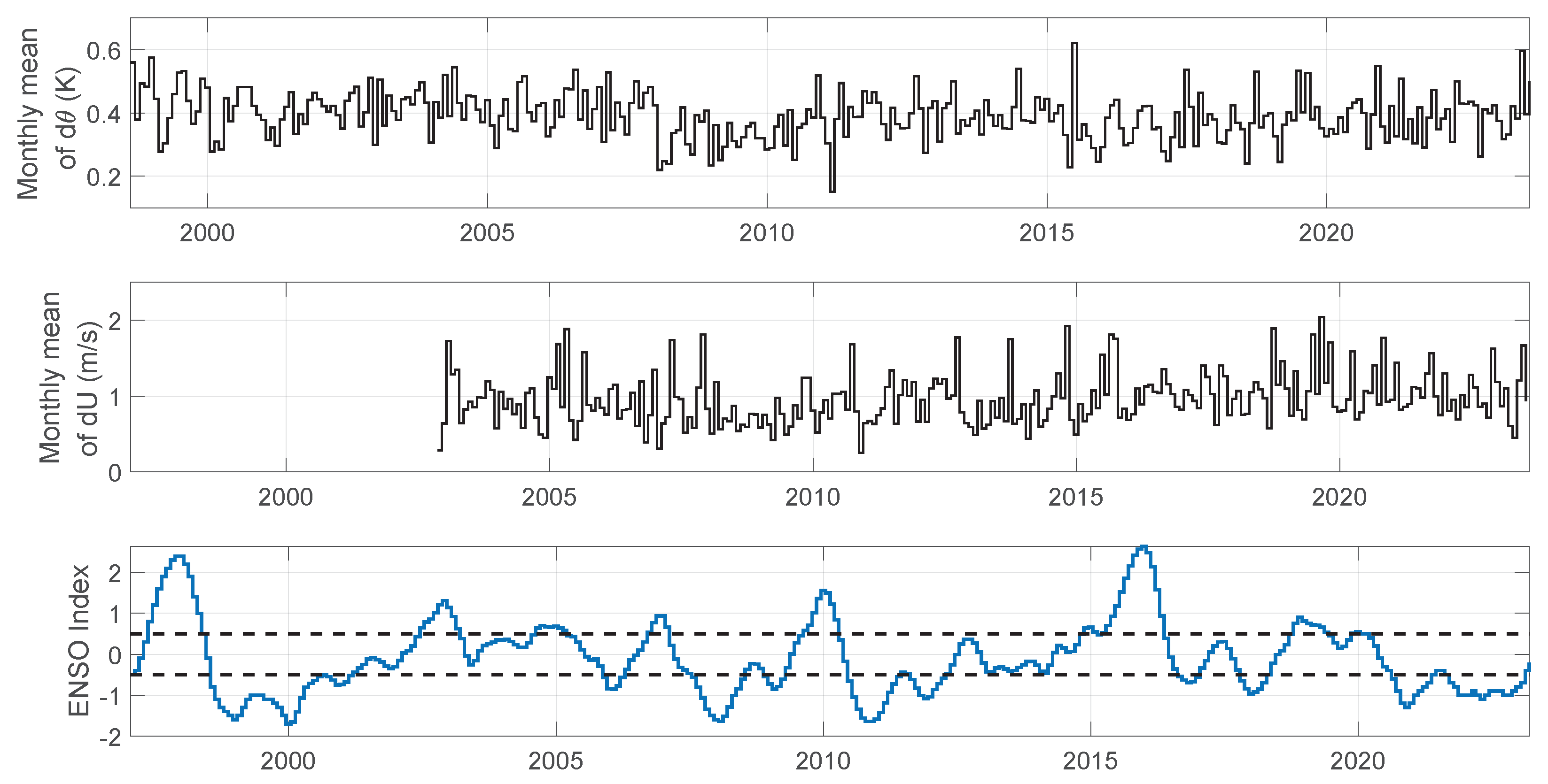
Furthermore, and motivated by the work of [37], we analysed the near surface level temperature record to check for possible trends in temperature gradients between the 30 m and 2 m height from the ground level. Similarly, we also analysed the vertical gradient in the horizontal wind speed from wind measurements performed at 30 m and 10 m above ground level. The long-term record for the monthly means of the vertical differences in temperature and horizontal wind speed are shown in Figure 6. Our results show seasonal variability, but, overall, the temperature and horizontal wind speed gradient have remained stable, within their natural variability. For completeness, the gradients are shown together with the ENSO index. This result on the wind speed and temperature gradient expands the exhaustive work on the relation of seeing and wind speed and temperature gradients in the context of climate change from 2009 at the Paranal Observatory [7]. In that work, the authors analysed the data from 1990 to 1998 and from 1998 to 2008 and concluded that climate change had no significant impact on seeing in this time period. Additionally, and most importantly, they concluded that the Armazones site, now host of the ELT construction, was unaffected both by seeing changes due to climate change or due to EN or LN phases. We expand their findings with complementary data from the decade following their study.

To better understand the potential impact of ENSO on seeing, we studied the seeing during the night, separating out especially strong EN/LN phases (see Appendix B-

Table A6. Spread of seeing for strong EN phases ($\delta T>0.75{}^{\circ }\mathrm{C}$).

Period	Variance	75–25%	95–5%
2-July to December	$0.13$	$0.42$	$1.14$
6-October to November	$0.28$	$0.55$	$1.64$
9-October to 10-February	$0.20$	$0.47$	$1.37$
15-May to 16-March	$0.19$	$0.50$	$1.36$

and

Table A7. Spread of seeing for strong LN phases ($\delta T<-0.75{}^{\circ }\mathrm{C}$).

Period	Variance	75–25%	95–5%
98-July to 00-March	$0.19$	$0.45$	$1.39$
5-December to 6-January	$0.13$	$0.40$	$1.12$
7-August to 8-April	$0.24$	$0.59$	$1.46$
8-December to 9-January	$0.24$	$0.55$	$1.46$
10-July to 11-February	$0.34$	$0.54$	$1.66$
11-September to 11-December	$0.18$	$0.48$	$1.27$
17-November to 18-January	$0.12$	$0.33$	$1.10$
20-September to 21-February	$0.13$	$0.38$	$1.12$

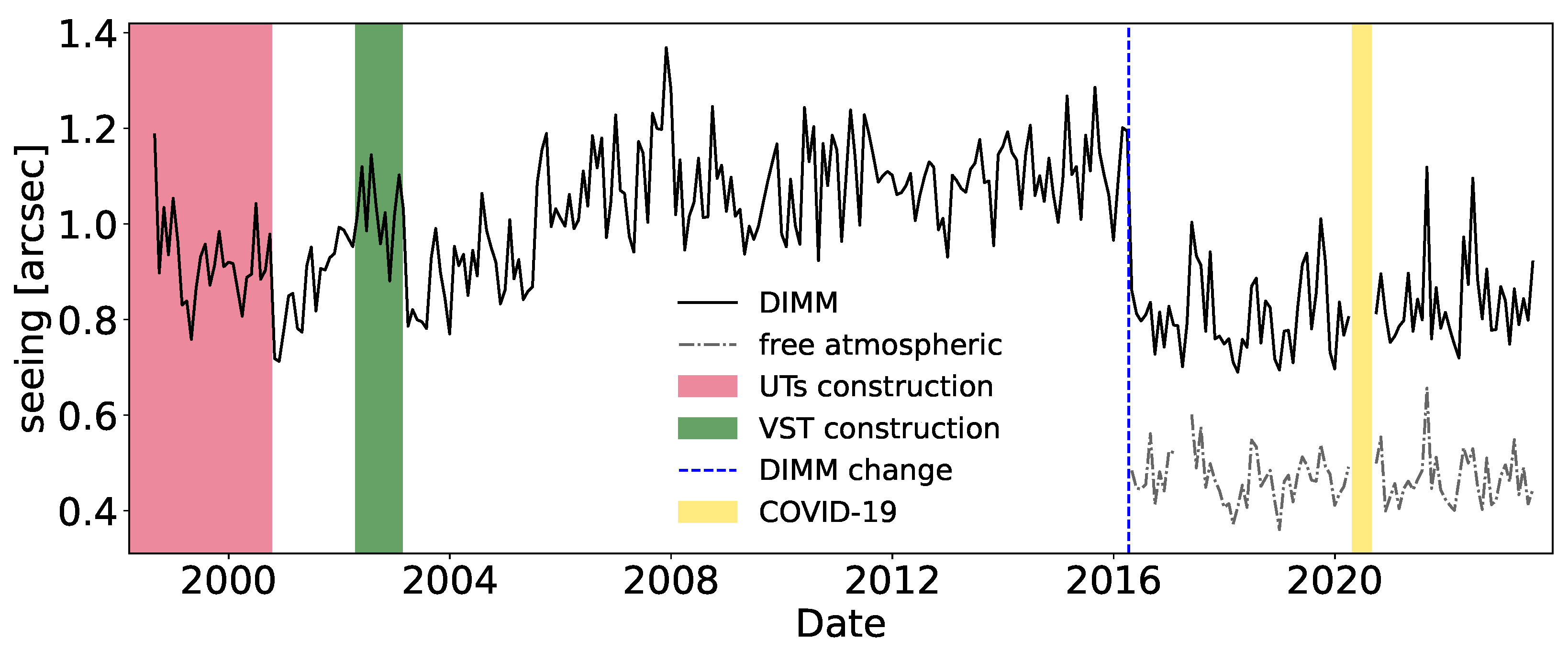
) and found no significant difference in seeing, although dry EN phases showed less variance in seeing. Figure 7 shows the seeing at the Paranal Observatory in the period 1998–2023. This time series is affected by biases induced by construction and the proximity of the telescope buildings to the former seeing monitor tower (1998-April 2016) [37], a position prone to the influence of surface-layer turbulence re-circulation. The new seeing monitor instrument (DIMM) was then moved away from the telescope building and raised up, from 5 m above ground level to 7 m. Due to this improvement, the seeing came back to the best long-term values before construction, showing that no gradual increase with time was taking place. In the latest record, we may see evidence of an increase in the lowest seeing values, but the time series is still too short to attempt a correlation with ENSO or climate change.

Moreover, we explored a possible trend between the surface-level turbulence differences between the EN and LN phases of ENSO via the Richardson number. Our results, derived from the data in Figure 6 and taking $\theta$ = 314 K in Equation (4), show a nearly constant long-term Richardson number of about 0.2–0.3, consistent with the earlier work of [7], and no differences between the EN and LN periods.

As well as the integrated (whole-atmosphere) seeing in Figure 7, we have included the free-atmosphere seeing from 2016 onwards, which does not show any particular trend either. Free-atmosphere seeing results from optical turbulence from 250 m onwards, away from the surface layer, up to the top of the troposphere. The MASS instrument allows measuring the free-atmosphere seeing [11], as well as other parameters important for observational astronomy.

The period after 2020 was associated with LN conditions, and our results, as shown in Appendix B, indicate a higher seeing variability during LN periods. As we are entering (2023) into the next EN period, the future record of seeing will show if the lowest seeing conditions decrease compared to the 2016–2020 period characterised by mainly neutral ENSO conditions. Nonetheless, it is important to state that the seeing conditions in the Paranal and Cerro Armazones region (ELT site) remain exceptional for seeing-limited astronomical observations and, at large, are unaffected by ENSO and climate change, confirming the results from a decade prior [7].

4. Conclusions

From the analysis of meteorological data gathered at the European Southern Observatory sites, we found a positive correlation of extremely surface-level warm periods with ENSO across all sites, as well as an anti-correlation between ENSO and the surface-level absolute humidity. In other words, during EN phases, there was a high likelihood of warmer and dryer surface conditions. Similarly, during LN, the surface meteorological conditions call for lower maximum daily temperatures but higher absolute humidity. As a consequence, we now, for the first time, have predicting capabilities to better schedule more demanding infrared observation programs that cannot be executed in elevated humidity. Conversely, during LN phases, when periods of wet and cloudy conditions are more probable, we can plan for less restrictive programs.

Unrelated to astronomy, we confirm the overall trend of increasing temperatures for all sites with rates of about or more than 0.2 ${}^{\circ }$C/decade which are consistent with anthropogenic climate change since 1980. Our results show a significant increase in temperatures at the Chajnantor site in line with the acceleration of warming with altitude. These long-term, high-altitude stations built for astronomy could potentially become an important resource for the climate community as they fill an important gap in station coverage [38]. Regarding precipitable water vapour, our data for the Paranal Observatory do not show an increase in any metrics with time, confirming studies that have been conducted at the Chajnantor site.

While the trend in the absolute surface air temperature is evident, our results do not show a long-term trend in the vertical gradient of air temperature close to the surface, nor in the vertical gradient of the horizontal component of wind speed. Their ratios, following the formalism of the Richardson number, do not show a long trend or significant differences between strong phases of ENSO either, implying that the ground-level turbulence has remained within its natural seasonal variability, in line with previously conducted studies on seeing.

Regarding a possible trend in astronomical seeing since then, unfortunately, our long-term dataset for the Paranal Observatory is affected by biases that are hard to correct without introducing systematic errors. Nonetheless, we find no evidence for an increase in seeing or turbulence with time, contrary to popular beliefs on astronomical data quality over time. However, it seems that the spread in seeing is larger during strong LN phases, making conditions during LN even more unpredictable. The record of seeing in the following years will help elucidate a more direct impact of strong EN and LN events on seeing and we will discuss any visible trends in follow-up work. Additionally, the impact of the dome seeing on astronomical observations is not currently well studied and should be measured systematically in the future.

In conclusion, our work serves to confirm the increasing warming trend with altitude due to global warming, underscoring the unique exposure of observatory sites to the challenges that lie ahead. Despite not finding any direct impact on seeing yet, our research contributes valuable insights for observatories in their preparation for the challenging future climatic conditions, as well as a predictive tool via the ENSO phases for the scheduling of challenging near-infrared programmes.

References

1. Rutllant, J.A.; Fuenzalida, H.; Aceituno, P. Climate dynamics along the arid northern coast of Chile: The 1997–1998 Dinámica del Clima de la Región de Antofagasta (DICLIMA) experiment. J. Geophys. Res. Atmos. 2003, 108, 4538. [Google Scholar] [CrossRef]
2. Muñoz, R.C.; Zamora, R.A.; Rutllant, J.A. The Coastal Boundary Layer at the Eastern Margin of the Southeast Pacific (23.4°S, 70.4°W): Cloudiness-Conditioned Climatology. J. Clim. 2011, 24, 1013–1033. [Google Scholar] [CrossRef]
3. Schöck, M.; Els, S.; Riddle, R.; Skidmore, W.; Travouillon, T.; Blum, R.; Bustos, E.; Chanan, G.; Djorgovski, S.G.; Gillett, P.; et al. Thirty Meter Telescope Site Testing I: Overview. Publ. Astron. Soc. Pac. 2009, 121, 384. [Google Scholar] [CrossRef]
4. Vernin, J.; Muñoz-Tuñón, C.; Sarazin, M.; Vazquez Ramió, H.; Varela, A.M.; Trinquet, H.; Delgado, J.M.; Jiménez Fuensalida, J.; Reyes, M.; Benhida, A.; et al. European Extremely Large Telescope Site Characterization I: Overview. Publ. Astron. Soc. Pac. 2011, 123, 1334. [Google Scholar] [CrossRef]
5. Bustos, R.; Rubio, M.; Otarola, A.; Nagar, N. Parque Astronómico de Atacama: An Ideal Site for Millimeter, Submillimeter, and Mid-Infrared Astronomy. Publ. Astron. Soc. Pac. 2014, 126, 1126–1132. [Google Scholar] [CrossRef]
6. Otarola, A.; Richter, M.; Packham, C.; Chun, M. Atmospheric transmission and thermal background emission in the mid-infrared at Maunakea. J. Phys. Conf. Ser. 2015, 595, 012023. [Google Scholar] [CrossRef]
7. Melnick, J.; Sarazin, M.; Lombardi, G.L.; Navarrete, J. The Paranal surface layer. In Proceedings of the Optical Turbulence Meets Meteorology, Alghero, Italy, 15–18 September 2008; pp. 136–143. [Google Scholar] [CrossRef]
8. Montecinos, A.; Aceituno, P. Seasonality of the ENSO-Related Rainfall Variability in Central Chile and Associated Circulation Anomalies. J. Clim. 2003, 16, 281–296. [Google Scholar] [CrossRef]
9. Rojas-Murillo, K.; Lupo, A.R.; Garcia, M.; Gilles, J.; Korner, A.; Rivera, M.A. ENSO and PDO related interannual variability in the north and east-central part of the Bolivian Altiplano in South America. Int. J. Climatol. 2022, 42, 2413–2439. [Google Scholar] [CrossRef]
10. Sarazin, M.; Roddier, F. The ESO differential image motion monitor. Astron. Astrophys. 1990, 227, 294–300. [Google Scholar]
11. Tokovinin, A.; Kornilov, V. Accurate seeing measurements with MASS and DIMM. Mon. Not. R. Astron. Soc. 2007, 381, 1179–1189. [Google Scholar] [CrossRef]
12. Kerber, F.; Rose, T.; Chacón, A.; Cuevas, O.; Czekala, H.; Hanuschik, R.; Momany, Y.; Navarrete, J.; Querel, R.R.; Smette, A.; et al. A water vapour monitor at Paranal Observatory. In Proceedings of the Ground-Based and Airborne Instrumentation for Astronomy IV, Amsterdam, The Netherlands, 1–6 July 2012; Society of Photo-Optical Instrumentation Engineers (SPIE) Conference Series. McLean, I.S., Ramsay, S.K., Takami, H., Eds.; SPIE: Bellingham, WA, USA, 2012; Volume 8446, p. 84463. [Google Scholar] [CrossRef]
13. Cortés, F.; Cortés, K.; Reeves, R.; Bustos, R.; Radford, S. Twenty years of precipitable water vapor measurements in the Chajnantor area. Astron. Astrophys. 2020, 640, A126. [Google Scholar] [CrossRef]
14. Buck, A.L. New Equations for Computing Vapor Pressure and Enhancement Factor. J. Appl. Meteorol. 1981, 20, 1527–1532. [Google Scholar] [CrossRef]
15. Hunziker, S.; Gubler, S.; Calle, J.; Moreno, I.; Andrade, M.; Velarde, F.; Ticona, L.; Carrasco, G.; Castellón, Y.; Oria, C.; et al. Identifying, attributing, and overcoming common data quality issues of manned station observations. Int. J. Climatol. 2017, 37, 4131–4145. [Google Scholar] [CrossRef]
16. Kendall, M.G. Rank Correlation Methods. [Pp. vii + 160. London: Charles Griffin and Co. Ltd., 42 Drury Lane, 1948. 18s.]. J. Inst. Actuar. 1949, 75, 140–141. [Google Scholar] [CrossRef]
17. Yue, S.; Wang, C. The Mann-Kendall Test Modified by Effective Sample Size to Detect Trend in Serially Correlated Hydrological Series. Water Resour. Manag. 2004, 3, 201–218. [Google Scholar] [CrossRef]
18. Hussain, M.; Mahmud, I. pyMannKendall: A python package for non parametric Mann Kendall family of trend tests. J. Open Source Softw. 2019, 4, 1556. [Google Scholar] [CrossRef]
19. Sen, P.K. Estimates of the Regression Coefficient Based on Kendall’s Tau. J. Am. Stat. Assoc. 1968, 63, 1379–1389. [Google Scholar] [CrossRef]
20. Gómez-Fontealba, C.; Flores-Aqueveque, V.; Alfaro, S.C. Teleconnection between the Surface Wind of Western Patagonia and the SAM, ENSO, and PDO Modes of Variability. Atmosphere 2023, 14, 608. [Google Scholar] [CrossRef]
21. Thompson, D.W.J.; Wallace, J.M. Annular Modes in the Extratropical Circulation. Part I: Month-to-Month Variability. J. Clim. 2000, 13, 1000–1016. [Google Scholar] [CrossRef]
22. Mantua, N.J.; Hare, S.R.; Zhang, Y.; Wallace, J.M.; Francis, R.C. A Pacific Interdecadal Climate Oscillation with Impacts on Salmon Production. Bull. Am. Meteorol. Soc. 1997, 78, 1069–1079. [Google Scholar] [CrossRef]
23. Smith, C.A.; Sardeshmukh, P.D. The effect of ENSO on the intraseasonal variance of surface temperatures in winter. Int. J. Climatol. 2000, 20, 1543–1557. [Google Scholar] [CrossRef]
24. Garreaud, R.D.; Vuille, M.; Compagnucci, R.; Marengo, J. Present-day South American climate. Palaeogeogr. Palaeoclimatol. Palaeoecol. 2009, 281, 180–195. [Google Scholar] [CrossRef]
25. Böhm, C.; Reyers, M.; Schween, J.H.; Crewell, S. Water vapor variability in the Atacama Desert during the 20th century. Glob. Planet. Chang. 2020, 190, 103192. [Google Scholar] [CrossRef]
26. Pepin, N.C.; Maeda, E.E.; Williams, R. Use of remotely sensed land surface temperature as a proxy for air temperatures at high elevations: Findings from a 5000 m elevational transect across Kilimanjaro. J. Geophys. Res. Atmos. 2016, 121, 9998–10015. [Google Scholar] [CrossRef]
27. Haslebacher, C.; Demory, M.E.; Demory, B.O.; Sarazin, M.; Vidale, P.L. Impact of climate change on site characteristics of eight major astronomical observatories using high-resolution global climate projections until 2050. Projected increase in temperature and humidity leads to poorer astronomical observing conditions. Astron. Astrophys. 2022, 665, A149. [Google Scholar] [CrossRef]
28. Burger, F.; Brock, B.; Montecinos, A. Seasonal and elevational contrasts in temperature trends in Central Chile between 1979 and 2015. Glob. Planet. Chang. 2018, 162, 136–147. [Google Scholar] [CrossRef]
29. Rangwala, I.; Miller, J.R. Climate change in mountains: A review of elevation-dependent warming and its possible causes. Clim. Chang. 2012, 114, 527–547. [Google Scholar] [CrossRef]
30. Masiokas, M.H.; Christie, D.A.; Le Quesne, C.; Pitte, P.; Ruiz, L.; Villalba, R.; Luckman, B.H.; Berthier, E.; Nussbaumer, S.U.; González-Reyes, Á.; et al. Reconstructing the annual mass balance of the Echaurren Norte glacier (Central Andes, 33.5° S) using local and regional hydroclimatic data. Cryosphere 2016, 10, 927–940. [Google Scholar] [CrossRef]
31. Gilmozzi, R.; Spyromilio, J. The European Extremely Large Telescope (E-ELT). Messenger 2007, 127, 11. [Google Scholar]
32. Garreaud, R.D. The Climate of northern Chile: Mean state, variability and trends. In Proceedings of the Revista Mexicana de Astronomia y Astrofisica Conference Series, Astronomical Site Testing Data in Chile, Valparaiso, Chile, 1–3 December 2010; Revista Mexicana de Astronomia y Astrofisica Conference Series. Volume 41, pp. 5–11. [Google Scholar]
33. Krishnamurti, T.N.; Martin, A.; Krishnamurti, R.; Simon, A.; Thomas, A.; Kumar, V. Impacts of enhanced CCN on the organization of convection and recent reduced counts of monsoon depressions. Clim. Dyn. 2013, 41, 117–134. [Google Scholar] [CrossRef]
34. Segura, H.; Espinoza, J.C.; Junquas, C.; Lebel, T.; Vuille, M.; Garreaud, R. Recent changes in the precipitation-driving processes over the southern tropical Andes/western Amazon. Clim. Dyn. 2020, 54, 2613–2631. [Google Scholar] [CrossRef]
35. Ciddor, P.E. Refractive index of air: New equations for the visible and near infrared. Appl. Opt. 1996, 35, 1566. [Google Scholar] [CrossRef] [PubMed]
36. Thayer, G.D. An improved equation for the radio refractive index of air. Radio Sci. 1974, 9, 803–807. [Google Scholar] [CrossRef]
37. Cantalloube, F.; Milli, J.; Böhm, C.; Crewell, S.; Navarrete, J.; Rehfeld, K.; Sarazin, M.; Sommani, A. The impact of climate change on astronomical observations. Nat. Astron. 2020, 4, 826–829. [Google Scholar] [CrossRef]
38. Mutz, S.G.; Scherrer, S.; Muceniece, I.; Ehlers, T.A. Twenty-first century regional temperature response in Chile based on empirical-statistical downscaling. Clim. Dyn. 2021, 56, 2881. [Google Scholar] [CrossRef]
39. Falvey, M.; Garreaud, R.D. Regional cooling in a warming world: Recent temperature trends in the southeast Pacific and along the west coast of subtropical South America (1979–2006). J. Geophys. Res. Atmos. 2009, 114, D04102. [Google Scholar] [CrossRef]
Figure 1. Monthly median PWV at the Paranal Observatory. No significant incremental trends for minimum PWV are discernible. However, for the annual minimum PWV, a marginal seasonal pattern on a decadal scale might be inferred. This pattern remains statistically non-significant.
Atmosphere 14 01511 g001
Figure 2. Days in a month with the ambient temperature at 2 m above surface above the long-term 90th percentile for all sites studied. Values below the thresholds are shaded in blue, and values above the threshold are shaded in red. The lowest two panels show the Niño3.4 index and the PDO (Pacific Decadal Oscillation) index.
Atmosphere 14 01511 g002
Figure 3. The El Niño3.4 anomaly is shown in yellow with the number of days with sunset temperature above the 90th quantile (red line) and the WVD (blue dot) overlaid on the same scale as EN3.4 for the Paranal Observatory. The WVD is displayed as the wettest yearly period, the month each year with the highest mean WVD. A clear correlation is visible between positive ENSO anomalies and extremely warm and dry periods.
Atmosphere 14 01511 g003
Figure 4. The fraction of the year where the sunset air temperature at 2 m is above 16 C as black dots, expanding Figure 1c from [37], which spanned the years 2008–2020. The magenta line marks a linear fit to the data to indicate the long-term trend.
Atmosphere 14 01511 g004
Figure 5. Mean seeing probability density function (PDF) from Table A5 comparing morning and evening seeing on the left and the same normalised function for strong EN and LN events from Table A6 and Table A7. The PDF, on the right-hand side, is normalised such that all curves match the long-term median of seeing at the Paranal Observatory. The figure helps to compare the relative shapes of the probability density function curves.
Atmosphere 14 01511 g005
Figure 6. (top) Monthly means of the air temperature difference between measurements at 30 m and 2 m above ground level. (middle) Monthly means of the differences in the horizontal wind speed measured at 30 m and 10 m above ground level. The bottom plots, for completeness, show the time series of the El Niño index. Note: The trends of wind differences are shown starting in 2002. The wind record prior to 2002 shows some inconsistencies that produced a very small magnitude wind gradient. It is possible that the measurements for the period prior to 2002 were not performed exactly at the heights above ground as reported in the database, and, therefore, we opted to exclude this data.
Atmosphere 14 01511 g006
Figure 7. Mean monthly seeing at the Paranal Observatory with various important changes highlighted that impacted the mean seeing trend. No net increase in seeing is discernible at this stage.
Atmosphere 14 01511 g007