The Impact of Surface Waves and Spray Injection Velocities on Air–Sea Momentum and Heat Fluxes

Abstract

Surface waves and sea spray play a significant role in air–sea fluxes in high winds. The present study used a marine atmosphere surface layer (MASL), which couples the traditional Monin–Obukhov similarity theory, sea spray generation function, the balance of turbulent kinetic budget, and momentum/enthalpy conservation equations. Based on this model, the effects of wave states and spray injection velocities on air–sea momentum/enthalpy fluxes and near-surface wind/temperature profiles were theoretically investigated. Based on the assumption that the velocity of injected spray is the same as that of the ambient airflow, it was found that spray could increase the near-surface air turbulence intensity and inhibit air–sea fluxes at 10 m above the sea surface. Correspondingly, near-surface wind speeds and temperature increase in high winds. This phenomenon becomes prominent in cases of large wave ages or surface waves supporting a minority of air–sea fluxes. Based on the assumption that the velocity of the edges of breaking water bags is used to estimate that of spray injection, the opposite results were found: spray could weaken the near-surface air turbulence and increase total air–sea fluxes at 10 m above the sea surface. In this case, the near-surface wind speeds and temperature decreased. This reduction becomes remarkable when surface waves are full-developed or the majority of air–sea momentum fluxes are supported by waves.

1. Introduction

Air–sea interaction controls energy and mass transfer between the atmosphere and the ocean. It significantly affects the development of many atmospheric and oceanic systems, such as storm surges, ocean waves, and tropical cyclones [1,2,3]. Accurately modeling air–sea momentum and heat exchanges are crucial for understanding the physical processes in the marine atmosphere surface layer (MASL), particularly in conditions of high winds. Over the last decade, a good amount of research has been conducted on the impact of surface waves and sea spray on the MASL under tropical cyclones [4,5,6,7]. Nevertheless, some problems are still poorly understood and quantified. For example, some previous studies adopted the traditional Monin–Obukhov similarity theory to calculate momentum fluxes, though they failed to explicitly compute the momentum distribution among the airflow, surface waves, and sea spray [4,5]. Some studies did compute the momentum distribution, though their complicated mathematical expression was hardly applied to the numerical atmosphere or wave models [6,7]. Hence, I propose the use of mathematical expressions with a simple structure to compute the momentum distribution among near-surface airflow, surface waves, and spray droplets. Indeed, only less complicated expressions have the potential to be applied to operational models.

Spray droplets that are injected from the ocean surface to the airflow are divided into three categories according to the radii r, i.e., film, jet, and spume [8]. Generally, the spume droplets fall back to the ocean surface and affect the air–sea momentum and enthalpy fluxes. Some field and laboratory measurements found that air–sea momentum fluxes began to level off with wind speeds when surface winds were strong [9,10,11,12,13,14,15]. Spume droplets were regarded as the main interpretation for this phenomenon [16,17,18]. Additionally, a series of works studied the impact of spray on the thermodynamic structure of the MASL; however, their complicated derivation has hardly been verified by other researchers [19,20,21]. In another study, a one-dimensional model was proposed to couple the spray and MASL for the investigation of air–sea momentum and heat fluxes under high winds [22]. However, in their research, the bottom level of the model was so high that the processes that occurred near the air–sea interface were neglected. Recently, an artificial spray concentration was used to analyze the spray impact on vertical heat fluxes in the MASL [23]. The measured sea spray generation function (SSGF) measured from laboratories and fields is more accurate for characterizing the spray concentration.

Another body of research pointed out that some phenomena became more intensive in the MASL for surface winds exceeding 45 m s⁻¹, such as breaking waves, white capping, etc. [15,24,25]. Actually, surface waves and sea spray play crucial roles in the MASL for mean wind speeds stronger than 30 m s⁻¹ (defined as high winds) at 10 m above the sea surface. Some direct numerical simulations addressed the issue that air–sea momentum and heat transfer are sensitive to the horizontal injection velocity of spray droplets [26,27,28]. However, few discussions have been held about the impact of spray injection velocity on the distribution of momentum and heat fluxes among airflow, waves, and spray. This study used a theoretical model to investigate how the injection velocity of spray droplets affects the MASL. Based on the traditional Monin–Obukhov similarity theory (MOST), the modeling processes are divided into three steps. Firstly, according to a previous study [29], the spray impact was introduced into the budget equation of turbulent energy of near-surface airflow (TKE). This behavior altered the conventional Obukhov length of the MOST. Then, the wave-induced momentum flux and a spray source term with injection velocities were entered into the momentum conservation equation of the MASL. The addition of these two terms made the turbulent momentum flux in the MOST vary with height. Finally, the spray-induced sensible and latent heat fluxes obtained from laboratory experiments [30] were also introduced into the MOST. The remainder of this paper is organized as follows: the mathematical derivation of the model is presented in Section 2; designs and results of the numerical experiments are presented in Section 3; the discussion and conclusion are given in Section 4.

2. Mathematical Description of the MASL Model

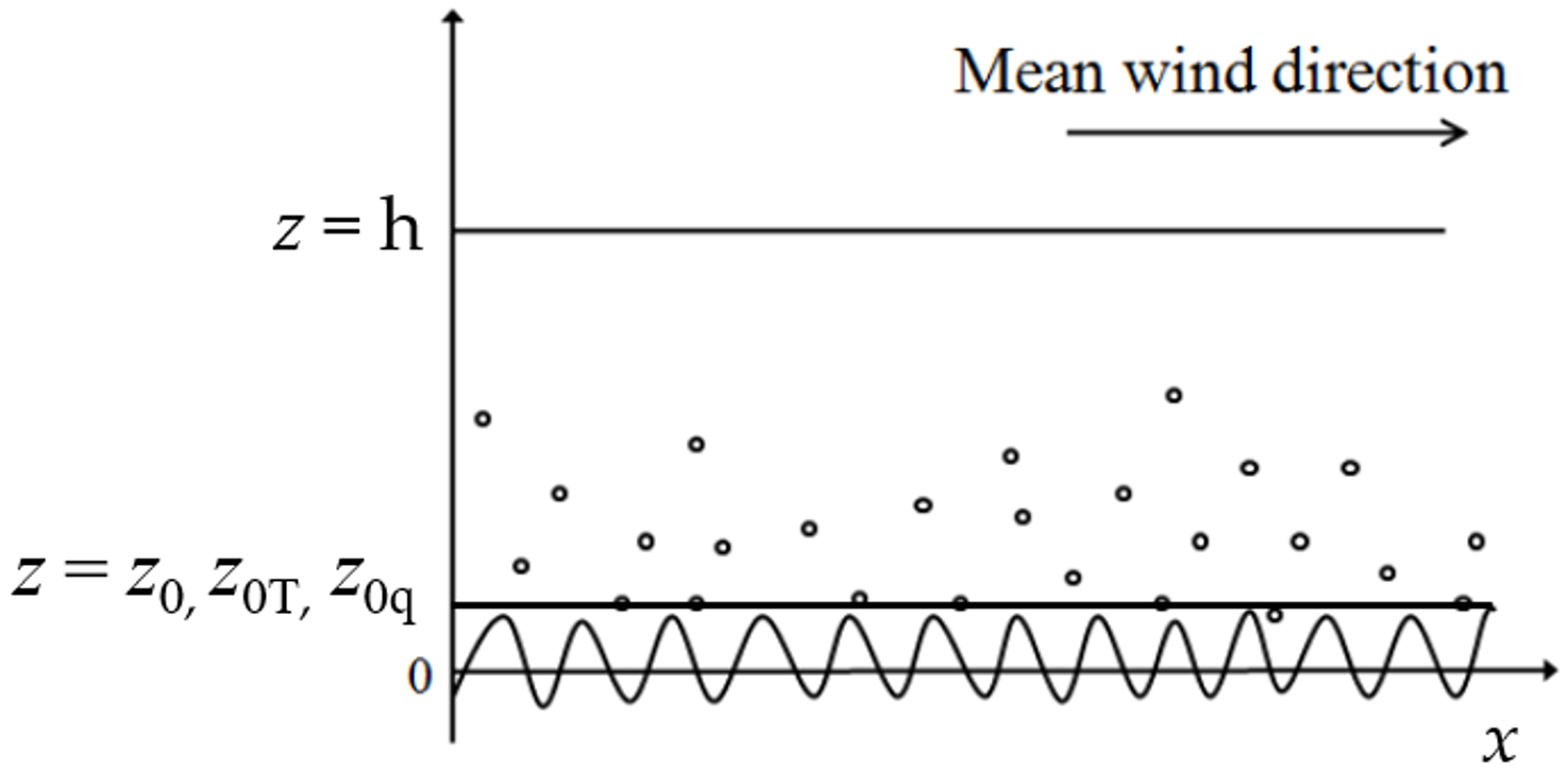
2.1. MOST for the Spray-Laden MASL

The spray-laden MASL model in this section was constructed according to a previous study [29]. For a detailed derivation of the model, please refer to that research paper. I supply a brief summary of the approach to modeling here. Accounting for the spray impact on both the buoyancy production and the TKE dissipation, the MOST used to describe the spray-laden MASL is written as follows [29]:

$$\frac{kz\sqrt{-\langle uw\rangle }}{-\langle uw\rangle }\frac{\partial U}{\partial z}={\phi }_{\mathrm{m}}\left(\frac{z}{L}\right),$$

(1)

$$\frac{kz\sqrt{-\langle uw\rangle }}{-\langle \theta w\rangle }\frac{\partial \Theta }{\partial z}={\phi }_{\mathrm{h}}\left(\frac{z}{L}\right),$$

(2)

$$\frac{kz\sqrt{-\langle uw\rangle }}{-\langle qw\rangle }\frac{\partial Q}{\partial z}={\phi }_{\mathrm{c}}\left(\frac{z}{L}\right),$$

(3)

where $k$ is the von Kármán constant; $z$ is the vertical coordinate (upward); $\langle .\rangle$ is the Reynolds averaging; $u$ and $w$, respectively, denote the fluctuation components of the horizontal and vertical air motions; $U$ is the mean horizontal velocity of air motions; $\Theta$ and $\theta$ are the mean and fluctuation components of potential temperature, respectively; $Q$ and $q$ are the mean and fluctuation components of specific humidity, respectively; and $L$ is the Obukhov length with spray impact. Under stable stratification, the universal functions ${\phi }_{\mathrm{m}}$, ${\phi }_{\mathrm{h}}$, and ${\phi }_{\mathrm{c}}$ on the right side of Equations (1)–(3) could be approximated in the following form [29,31,32]:

$$\phi =\mathsf{\alpha }+\mathsf{\beta }\frac{z}{L} ,$$

(4)

where the determination of constants $\mathsf{\alpha }$ and $\mathsf{\beta }$ depends on observations. Previous results have shown that they satisfied $0.74\le \mathsf{\alpha }\le 1$ and $4.7\le \mathsf{\alpha }\le 7.8$ [31,32]. Generally, $\mathsf{\alpha }=1$ and $\mathsf{\beta }=6$ are used for calculation [32]. In addition, $L^{-1}=L_{\mathrm{MO}}^{-1}+L_{\mathrm{SP}}^{-1}$, where $L_{\mathrm{MO}}^{}$ is the conventional Monin–Obukhov length and $L_{\mathrm{SP}}^{}$ is the spray-induced length. On the assumption that $uw$, $\theta w$, and $qw$ are constant in the MASL, by substituting Equation (4) into Equations (1)–(3) and integrating them from the reference height to local altitude z, the following relations could be obtained:

$$u_{*}=\frac{k\left[U\left(z\right)-U\left(z_0\right)\right]}{\ln \left(z/z_0\right)-{\Psi }_{\mathrm{m}}\left(z/L\right)},$$

(5)

$$-\frac{\langle \theta w\rangle }{u_{*}}=\frac{k\left[\Theta \left(z\right)-\Theta \left(z_{0\mathrm{T}}\right)\right]}{\ln \left(z/z_{0\mathrm{T}}\right)-{\Psi }_{\mathrm{h}}\left(z/L\right)},$$

(6)

$$-\frac{\langle qw\rangle }{u_{*}}=\frac{k\left[Q\left(z\right)-Q\left(z_{0\mathrm{q}}\right)\right]}{\ln \left(z/z_{0\mathrm{q}}\right)-{\Psi }_{\mathrm{h}}\left(z/L\right)},$$

(7)

where $u_{*}=\sqrt{-\langle uw\rangle }$ is the air friction velocity; $z_0$, $z_{0\mathrm{T}}$, and $z_{0\mathrm{q}}$ are the reference height for the zero mean wind speed, surface temperature, and moisture, respectively. The heights $z_0$, $z_{0\mathrm{T}}$, and $z_{0\mathrm{q}}$ denote the interface between water and air. In other words, they denote the bottom of the MASL model. The mean wind speed, temperature, and moisture at these heights satisfy $U(z_0)=0$, $\Theta (z_{0\mathrm{T}})=$ sea surface temperature, and $Q\left(z_{0\mathrm{q}}\right)=$ sea surface moisture (see Figure 1). The terms ${\Psi }_{\mathrm{m}}$ and ${\Psi }_{\mathrm{h}}$ on the right side of Equations (5)–(7) are stability functions, which are partitioned into two parts, i.e.,

$${\Psi }_{\mathrm{m}}\left(z/L\right)={\Psi }_{\mathrm{m}}{}^{\left(1\right)}\left(z/L_{\mathrm{MO}}\right)+{\Psi }_{\mathrm{m}}{}^{\left(2\right)}\left(z/L_{\mathrm{SP}}\right),$$

(8)

$${\Psi }_{\mathrm{h}}\left(z/L\right)={\Psi }_{\mathrm{h}}{}^{\left(1\right)}\left(z/L_{\mathrm{MO}}\right)+{\Psi }_{\mathrm{h}}{}^{\left(2\right)}\left(z/L_{\mathrm{SP}}\right),$$

(9)

in which the superscripts (1) and (2), respectively, denote the functions of $z/L_{\mathrm{MO}}$ and $z/L_{\mathrm{SP}}$_. In high winds, the impact of spray loading due to gravity plays a significant role in the Obukhov length $L$ so that the $L_{\mathrm{MO}}{}^{-1}$ is negligible compared with $L_{\mathrm{SP}}{}^{-1}$, and the terms with superscripts (1) could be neglected, meaning that Equations (8) and (9) become

$${\Psi }_{\mathrm{m}}\left(z/L\right)\approx {\Psi }_{\mathrm{m}}{}^{\left(2\right)}\left(z/L_{\mathrm{SP}}\right),$$

(10)

$${\Psi }_{\mathrm{h}}\left(z/L\right)\approx {\Psi }_{\mathrm{h}}{}^{\left(2\right)}\left(z/L_{\mathrm{SP}}\right),$$

(11)

where the detailed information on the right-side term could refer to the ${\mathsf{\Psi }}_{\mathrm{s}}$ of Equation (4.1) in this paper [29].

2.2. Momentum and Enthalpy Conservation Equations of the Spray-Laden MASL

2.2.1. Momentum Conservation Equation

The previous hypothesis regarded that the turbulent momentum flux did not vary with height [29]. This indicates that the momentum flux was only distributed in the airflow of the MASL. In this study, a different assumption is given. Part of the momentum at a lower altitude of the MASL is transported from the airflow to surface waves and sea spray. That is to say, at the lower MASL, the momentum fluxes are distributed among airflow, surface waves, and sea spray. At the top of the MASL, the momentum was only supported by airflow due to the slight effects of surface waves and spray droplets. Thus, the turbulent momentum flux varies with height rather than a constant in the MASL. This assumption is reasonable due to the spray concentration being greater at the lower MASL. Recent results of large-eddy simulations also revealed that the turbulent momentum varied with height in the lower MASL [24], which supports the assumption made in this study. Considering that spray droplets also bring momentum into the airflow once they are torn off from breaking waves, a volume source of spray momentum should be included in the MASL [33]. Here, the “spray source term” with the injection velocity was added to the momentum conservation equation as follows:

$$\frac{\partial }{\partial z}\left[{\rho }_{\mathrm{a}}\langle uw\rangle -{\rho }_{\mathrm{w}}{U}_{\mathrm{inj}}\left(z\right)F_{\mathrm{S}}\left(z\right)\right]={\rho }_{\mathrm{w}}{U}_{\mathrm{inj}}\left(z\right)V_{\mathrm{S}}\left(z\right),$$

(12)

where ${\rho }_{\mathrm{a}}$ and ${\rho }_{\mathrm{w}}$ denote the densities of the air and water, respectively; $U_{\mathrm{inj}}\left(z\right)$ is the horizontal injection velocity of spray droplets; $V_{\mathrm{S}}\left(z\right)$ is the total volume of the spray injected into the airflow per second per unit volume of the air; and $F_{\mathrm{S}}\left(z\right)$ is the spray volume flux, which was estimated as follows:

$$F_{\mathrm{S}}\left(z\right)={{\displaystyle \int }}_z^{+\infty }{V}_{\mathrm{S}}\left(z’\right)\mathrm{d}z’.$$

Note that the term $V_{\mathrm{S}}$ simulates the spray generation by the horizontal wind tearing off the crests of breaking waves. Hence, this study states that the horizontal injection velocity is approximately stronger than the vertical one so the latter could be negligible. Additionally, spray droplets being torn off from breaking waves are assumed to be injected into the airflow at the altitude of breaking wave crests. Hence, the injection velocity $U_{\mathrm{inj}}$ is a function of the height z. The second term ${\rho }_{\mathrm{w}}{U}_{\mathrm{inj}}\left(z\right)F_{\mathrm{S}}\left(z\right)$ on the left side of Equation (12) depicts the momentum flux transferred from the airflow to sea spray. In contrast, the term ${\rho }_{\mathrm{w}}{U}_{\mathrm{inj}}\left(z\right)V_{\mathrm{S}}\left(z\right)$ on the right side of Equation (12) depicts the momentum flux transferred from the spray to the airflow. Thus, Equation (12) characterizes the momentum balance resulting from the interaction between the sea spray and ambient airflow.

According to the existing experimental and theoretical research [30,34], the following mechanism by which spume droplets are generated in high winds is considered here. Due to this mechanism, before the formation of spray droplets, the near-surface airflow also transports momentum to the small-scale disturbances that arise at the water–air interface for their development from a small perturbation to water bags that separate droplets. The process, where a small piece of water is perturbated to split spray droplets, is called “water bag breakup”. In addition, as we know, non-breaking surface waves also participate in the regulation of the momentum in the MASL. Herewith, these two crucial fluxes are also incorporated in Equation (12) and are to be written as follows:

$$\frac{\partial }{\partial Z}\left[{\rho }_{\mathrm{a}}\langle uw\rangle -{\rho }_{\mathrm{w}}{U}_{\mathrm{inj}}\left(z\right)F_{\mathrm{S}}\left(z\right)-{\rho }_{\mathrm{w}}\langle U_{\mathrm{b}}\rangle F_{\mathrm{S}}\left(z\right)-{\tau }_{\mathrm{w}}\right]={\rho }_{\mathrm{w}}{U}_{\mathrm{inj}}\left(z\right)V_{\mathrm{S}}\left(z\right),$$

(13)

where the term ${\rho }_{\mathrm{w}}\langle U_{\mathrm{b}}\rangle F_{\mathrm{S}}\left(z\right)$ depicts the momentum flux due to the “water bag breakup”; $\langle U_{\mathrm{b}}\rangle =1.96+1.21u_{*}$. is the velocity of the edges of the breaking water bag; and the term ${\tau }_{\mathrm{w}}$ is the wave-induced momentum flux.

By integrating Equation (13) from z to the height $\mathrm{h}$, where the effects of the spray and waves are ignored, the following equation could be obtained:

$$-{\rho }_{\mathrm{a}}\langle uw\rangle +{\rho }_{\mathrm{w}}\left[\langle U_{\mathrm{b}}\rangle F_{\mathrm{S}}\left(z\right)+U_{\mathrm{inj}}\left(z\right)F_{\mathrm{S}}\left(z\right)-{{\displaystyle \int }}_{\mathrm{z}}^{\mathrm{h}}{V}_{\mathrm{S}}\left(z’\right)U_{\mathrm{inj}}\left(z’\right)\mathrm{d}z’\right]+{\tau }_{\mathrm{w}}={\rho }_{\mathrm{a}}{u}_{*}^2,$$

(14)

where $u_{*}^2$ is defined as the friction velocity at $\mathrm{h}$ and formulated as $u_{*}^2=-uw{|}_{\mathrm{h}}$, and the second term in the brackets of Equation (14) is defined as the spray-induced momentum flux in this study. It can be expressed as ${\tau }_{\mathrm{SP}}$ as follows:

$${\tau }_{\mathrm{SP}}={\rho }_{\mathrm{w}}\left[\langle U_{\mathrm{b}}\rangle F_{\mathrm{S}}\left(z\right)+U_{\mathrm{inj}}\left(z\right)F_{\mathrm{S}}\left(z\right)-{{\displaystyle \int }}_z^{\mathrm{h}}{V}_{\mathrm{S}}\left(z’\right)U_{\mathrm{inj}}\left(z’\right)\mathrm{d}z’\right],$$

(15)

in which the positive term $\langle U_{\mathrm{b}}\rangle F_{\mathrm{S}}\left(z\right)$ represents the momentum flux due to the spray generation, the positive term $U_{\mathrm{inj}}\left(z\right)F_{\mathrm{S}}\left(z\right)$ represents the momentum fluxes owning to the spray acceleration, and the last negative term $-{{\displaystyle \int }}_z^{\mathrm{h}}{V}_{\mathrm{S}}\left(z’\right)U_{\mathrm{inj}}\left(z’\right)\mathrm{d}z’$ denotes the momentum fluxes that the spray droplets give back to the airflow during their settlement. By regarding the $U_{\mathrm{inj}}\left(z\right)=\langle U_{\mathrm{b}}\rangle$ following paper [34], Equation (15) turns into the following:

$${\tau }_{\mathrm{SP}}={\rho }_{\mathrm{w}}\langle U_{\mathrm{b}}\rangle F_{\mathrm{S}}\left(z\right),$$

(16)

which was called “droplet stress” in that paper. In the present study, the injection velocity $U_{\mathrm{inj}}\left(z\right)$ is adopted in another two different cases to conduct a further investigation.

2.2.2. Enthalpy Conservation Equation

In high-wind conditions, the total air–sea enthalpy fluxes include two components [34], i.e., turbulent- and spray-mediated fluxes. The turbulent sensible and latent heat fluxes $H_{\mathrm{ts}}$ and $H_{\mathrm{tl}}$ are expressed as follows [4]:

$$H_{\mathrm{ts}}={\rho }_{\mathrm{a}}{c}_{\mathrm{pa}}{C}_{\mathrm{H}10}{U}_{10}\left(T_{\mathrm{s}}-T_{10}\right),$$

(17)

$$H_{\mathrm{tl}}={\rho }_{\mathrm{a}}{L}_{\mathrm{v}}{C}_{\mathrm{E}10}{U}_{10}\left(q_{\mathrm{s}}-q_{10}\right),$$

(18)

where $c_{\mathrm{pa}}$ is the specific heat of moist air; $L_{\mathrm{v}}$ is the latent heat of the vaporization of air; $C_{\mathrm{H}10}$ and $C_{\mathrm{E}10}$ are the exchange coefficients of sensible and latent heat fluxes at 10 m above mean sea level; $U_{10}$ is the 10 m wind speed; $T_{\mathrm{s}}$ and $q_{\mathrm{s}}$ are the surface temperature and moisture; and $T_{10}$ and $q_{10}$ are the temperature and moisture at 10 m.

The sensible and latent spray-mediated fluxes, which indicate that the heat transfers from spray to airflow, are evaluated by the following [34]:

$$H_{\mathrm{ss}}={{\displaystyle \int }}_{r_{\mathrm{L}}}^{r_{\mathrm{H}}}\left[\mathrm{d}F\left(r\right)/\mathrm{d}r\right]\left[c_{\mathrm{w}}{m}_0\left(T_{\mathrm{w}}-T_{\mathrm{sp}}\right)-L_{\mathrm{v}}\left(m_0-m_{\mathrm{f}}\right)\right]\mathrm{d}r,$$

(19)

$$H_{\mathrm{sl}}={{\displaystyle \int }}_{r_{\mathrm{L}}}^{r_{\mathrm{H}}}\left[\mathrm{d}F\left(r\right)/\mathrm{d}r\right]\left[L_{\mathrm{v}}\left(m_0-m_{\mathrm{f}}\right)\right]\mathrm{d}r,$$

(20)

where $F\left(r\right)$ is the SSGF; $r_{\mathrm{L}}$ and $r_{\mathrm{H}}$ are the lower and upper limits of the droplets’ radius; $c_{\mathrm{w}}$ is the specific heat of seawater; $L_{\mathrm{v}}$ is the latent heat of vaporization; $m_0=\left(4/3\right)\pi {\rho }_{\mathrm{w}}{r}_0^3$ and $m_{\mathrm{f}}=\left(4/3\right)\pi {\rho }_{\mathrm{w}}{r}_{\mathrm{f}}^3$ are the droplet masses at the moments of their injection and reentrance into the water, respectively; $T_{\mathrm{w}}$ is the surface temperature; and $T_{\mathrm{sp}}$ is the droplet temperature at its thermal equilibrium.

2.3. Introduction of New Fluxes to the MOST for Spray-Laden MASL

In this section, the momentum and enthalpy conservation equations in Section 2.2 are integrated into the MOST in Section 2.1. That is to say, fluxes due to spray and waves are added into the MOST. By substituting Equations (14) and (15) and Equations (17)–(20) into Equations (1)–(3), the MOST for the spray-laden MASL is written as follows:

$$\frac{kz{u}_{*}\left(z\right)}{u_{*}^2\left(z\right)}\frac{\partial U}{\partial z}={\phi }_{\mathrm{m}}\left(\frac{z}{L}\right),$$

(21)

$$-\frac{kz{u}_{*}\left(z\right)}{\langle {\theta }_{\mathrm{t}}w\rangle +\langle {\theta }_{\mathrm{sp}}w\rangle }\frac{\partial \Theta }{\partial z}={\phi }_{\mathrm{h}}\left(\frac{z}{L}\right),$$

(22)

$$-\frac{kz{u}_{*}\left(z\right)}{\langle q_{\mathrm{t}}w\rangle +\langle q_{\mathrm{sp}}w\rangle w}\frac{\partial Q}{\partial z}={\phi }_{\mathrm{c}}\left(\frac{z}{L}\right),$$

(23)

where the normalized momentum and enthalpy fluxes $u_{*}^2\left(z\right)$, $\langle {\theta }_{\mathrm{t}}w\rangle$, $\langle {\theta }_{\mathrm{sp}}w\rangle$, $\langle q_{\mathrm{t}}w\rangle$, and $\langle q_{\mathrm{sp}}w\rangle$ satisfy the following relationships:

$$u_{*}^2\left(z\right)={\mathsf{\rho }}_{\mathrm{a}}{u}_{*}^2-{\tau }_{\mathrm{sp}}-{\tau }_{\mathrm{w}}/{\rho }_{\mathrm{a}}, \langle {\theta }_{\mathrm{t}}w\rangle =H_{\mathrm{ts}}/{\rho }_{\mathrm{a}}, \langle {\theta }_{\mathrm{sp}}w\rangle =H_{\mathrm{ss}}/{\rho }_{\mathrm{a}},$$

$$\langle q_{\mathrm{t}}w\rangle =H_{\mathrm{tl}}/{\rho }_{\mathrm{w}}, \langle q_{\mathrm{sp}}w\rangle =H_{\mathrm{sl}}/{\rho }_{\mathrm{w}}.$$

(24)

Until now, the spray-laden MASL mathematically described by the MOST framework was completely constructed. It combined the TKE budget, momentum, and enthalpy conservation equations. Compared with the previous framework in Equations (1)–(3), the main innovation in Equations (21)–(23) is the introduction of the momentum and heat fluxes due to spray and waves. Notably, the $u_{*}$ in Equations (21)–(23) is no longer a constant with the height, and the equations could not be integrated to obtain simple forms like in Equations (5)–(7). Hence, the difference method and Newton iteration are applied here to compute Equations (21)–(23). In addition, surface drag and effective enthalpy coefficients (i.e., $C_{d10}$ and $C_{k10}$) are computed through the following laws [29]:

$$C_{\mathrm{d}10}={\left(u_{*}/U_{10}\right)}^2,$$

(25)

$$C_{\mathrm{k}10}=\left(H_{\mathrm{ts}}+H_{\mathrm{tl}}+H_{\mathrm{ss}}+H_{\mathrm{sl}}\right)/\left\{{\rho }_{\mathrm{a}}{U}_{10}\left[c_{\mathrm{pa}}\left(T_{\mathrm{s}}-T_{10}\right)+L_{\mathrm{v}}\left(q_{\mathrm{s}}-q_{10}\right)\right]\right\}.$$

(26)

2.4. Parameterizations

2.4.1. Sea Surface Roughness Length

Figure 1 shows the conceptual description of the spray-laden MASL. A Cartesian framework is located at the mean sea level; the x-axis orients along the mean wind direction and the z-axis is upward. The dynamic surface roughness $z_0$ significantly affects flux predictions in weather and climate models. Its parameterization has not been thoroughly uniform in all model configurations. A recent study revealed that the decrease in $z_0$ in the WRF (weather research and forecast) model led to significant improvements in the intensity forecasts of strong hurricanes [25]. In this study, the one-dimensional wave field is assumed to be parallel to the x-axis. Thus, the surface roughness length $z_0$ parameterized by ${\tau }_{\mathrm{w}}$ is applied here [35], i.e.,

$$z_0=\alpha u_{*}^2/\mathrm{g}, \alpha =c/\sqrt{1-x},$$

(27)

where g is the gravity acceleration; $x={\tau }_{\mathrm{w}}/u_{*}^2$ is the ratio parameter; and c = 0.001 is an empirical constant. The computation of ${\tau }_{\mathrm{w}}$ is primarily contributed by several parameters, e.g., wave spectra and growth/decay rates. These parameters have diverse formulations among numerical models and theoretical studies, which makes the determination of ${\tau }_{\mathrm{w}}$ continue to be challenging. Herewith, instead of using the specific formulation of ${\tau }_{\mathrm{w}}$, this study focuses on how the ratio parameter $x$ affects air–sea fluxes in high winds. The sign of $x$ is positive here since only wind waves are taken into consideration.

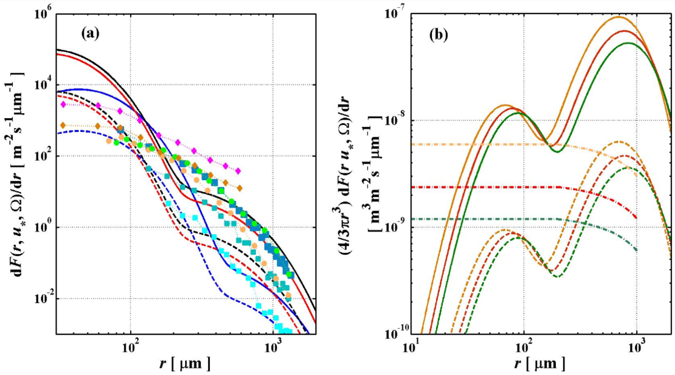
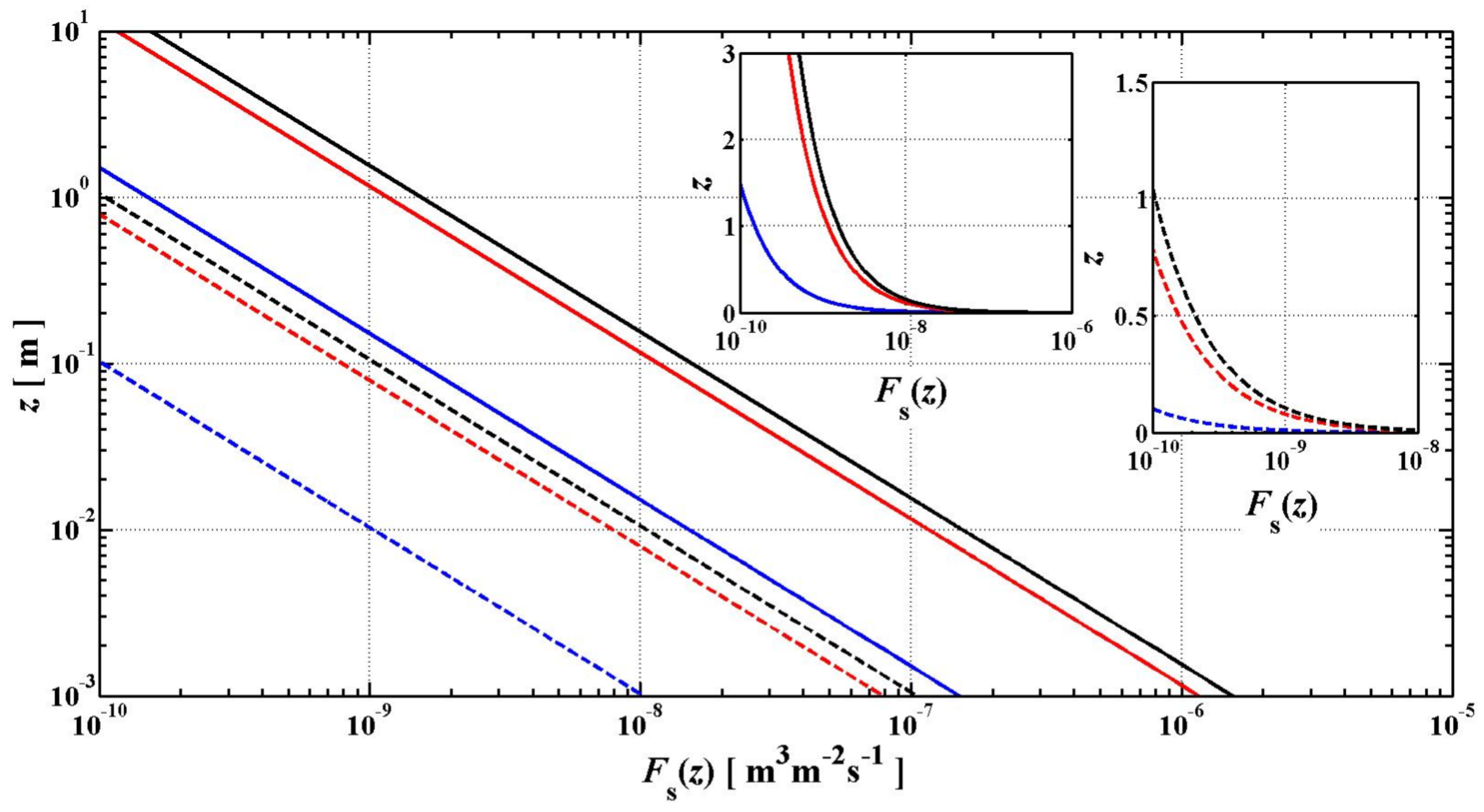
2.4.2. Spray-Induced Momentum Flux ${\tau }_{\mathrm{SP}}$

Equation (15) indicates that the evolution of spray-induced momentum flux depends on the spray volume flux $F_{\mathrm{S}}$; generally, it results from the SSGF integrated through the droplet radius, i.e.,

$$F_{\mathrm{S}}\left(z\right)=f\left(z\right){{\displaystyle \int }}_{r_{\mathrm{L}}}^{r_{\mathrm{H}}}\left(\frac{4}{3}\pi r^3\right)\left[\mathrm{d}F\left(r\right)/\mathrm{d}r\right],$$

(28)

where $F\left(r\right)$ is the SSGF and $f\left(z\right)$ is the decay function [29]. The state-of-the-art SSGF in the paper [34] is adopted here since the experiments found that giant droplets (r ~ 1000 μm) were produced at high winds. Here, the lower and upper limits of the spray radius in Equation (28) are $r_{\mathrm{L}}$ = 30 μm and $r_{\mathrm{H}}$ = 1500 μm, respectively. Under different wind speeds and wave states, the comparisons of SSGF in Equation (28), which were computed under different conditions, and others are shown in Figure 2a. Note that the wave state is characterized through the wave age $\mathsf{\Omega }$, which is less than the 1.0 generally used to parameterize wind waves. Figure 2b shows the comparison between computed spray volumes and previous theoretical results. The vertical profiles of spray volume flux $F_{\mathrm{S}}\left(z\right)$ in Equation (28) are shown in Figure 3, revealing that $F_S\left(z\right)$ decays with height more slowly when $U_{10}$ and $\mathsf{\Omega }$ are larger. The two subplots on the top-right corner indicate that the spray fluxes at 10 m are too small to be considered. It is reasonable to regard the top of the MASL to be 10 m above the sea surface.

3. Numerical Experiments and Results

This section is dedicated to comparing the simulated results in Section 2.1 and 2.3. Generally, the mean wind speed at 10 m above the sea surface was used to compute air–sea fluxes [34,39]. Some theoretical results revealed that surface waves and sea spray mainly influenced the airflow turbulent structure up to 10 m above the sea surface [6,7,33]. Thus, the top and bottom of the MASL were set at 10 m and $z_0$ m, respectively. Other control parameters to input into the models included 10 m wind speed $U_{10}$, wave-related ratio parameter $x$, and wave age $\mathsf{\Omega }$. The experimental designs are shown in

Table 1. Input values of 10 m wind speed, ratio parameter, and wave age to run the MASL model.

$10 \mathbf{m} \mathbf{Wind} \mathbf{Speed} {\mathit{U}}_{10}$ (m s−1)	$\mathbf{Ratio} \mathbf{Parameter} \mathit{x}$	$\mathbf{Wave} \mathbf{Age} \Omega$
30	0.95	0.2
30	0.95	0.6
30	0.95	1.0
30	0.05	0.2
30	0.05	0.6
30	0.05	1.0
50	0.95	0.2
50	0.95	0.6
50	0.95	1.0
50	0.05	0.2
50	0.05	0.6
50	0.05	1.0

and

Table 2. Input values of 10 m wind speed range, ratio parameter range, and wave age to run the MASL model.

$\mathbf{Wave} \mathbf{Age} \Omega$	$10 \mathbf{m} \mathbf{Wind} \mathbf{Speed} {\mathit{U}}_{10}$ (m s−1)	$\mathbf{Ratio} \mathbf{Parameter} \mathit{x}$
0.2	$2\le U_{10}\le 60$	$0.05\le x\le 0.45$
0.2	$2\le U_{10}\le 60$	$0.45\le x\le 0.75$
0.2	$2\le U_{10}\le 60$	$0.75\le x\le 0.95$
0.6	$2\le U_{10}\le 60$	$0.05\le x\le 0.45$
0.6	$2\le U_{10}\le 60$	$0.45\le x\le 0.75$
0.6	$2\le U_{10}\le 60$	$0.75\le x\le 0.95$
1.0	$2\le U_{10}\le 60$	$0.05\le x\le 0.45$
1.0	$2\le U_{10}\le 60$	$0.45\le x\le 0.75$
1.0	$2\le U_{10}\le 60$	$0.75\le x\le 0.95$

. $U_{10}$ is adopted as 30 m s⁻¹ and 50 m s⁻¹ to represent surface winds under typhoon and super typhoon conditions, respectively;$\mathsf{\Omega }$ is adopted as 0.2, 0.6, and 1.0 to represent the young, developing, and mature wind waves, respectively; and $x$ is adopted as $0.05$ and $0.95$ to characterize the low and high ocean energy contained in non-breaking waves, respectively. Similar physical meanings can be given to the three parameters in Table 2. To investigate the injection velocity of spray droplets on the model results, two cases are considered here. One case assumed that the injection velocity is equal to the wind speed at the same altitude, i.e., $U_{\mathrm{inj}}\left(z\right)=U\left(z\right)$. This indicates that once spray droplets are injected, they are simultaneously accelerated to the velocity of their surrounding airflow. The other case assumed that the injection velocity of spray droplets is the same as that of the edges of breaking water bags, i.e., $U_{\mathrm{inj}}\left(z\right)=\langle U_{\mathrm{b}}\rangle$.

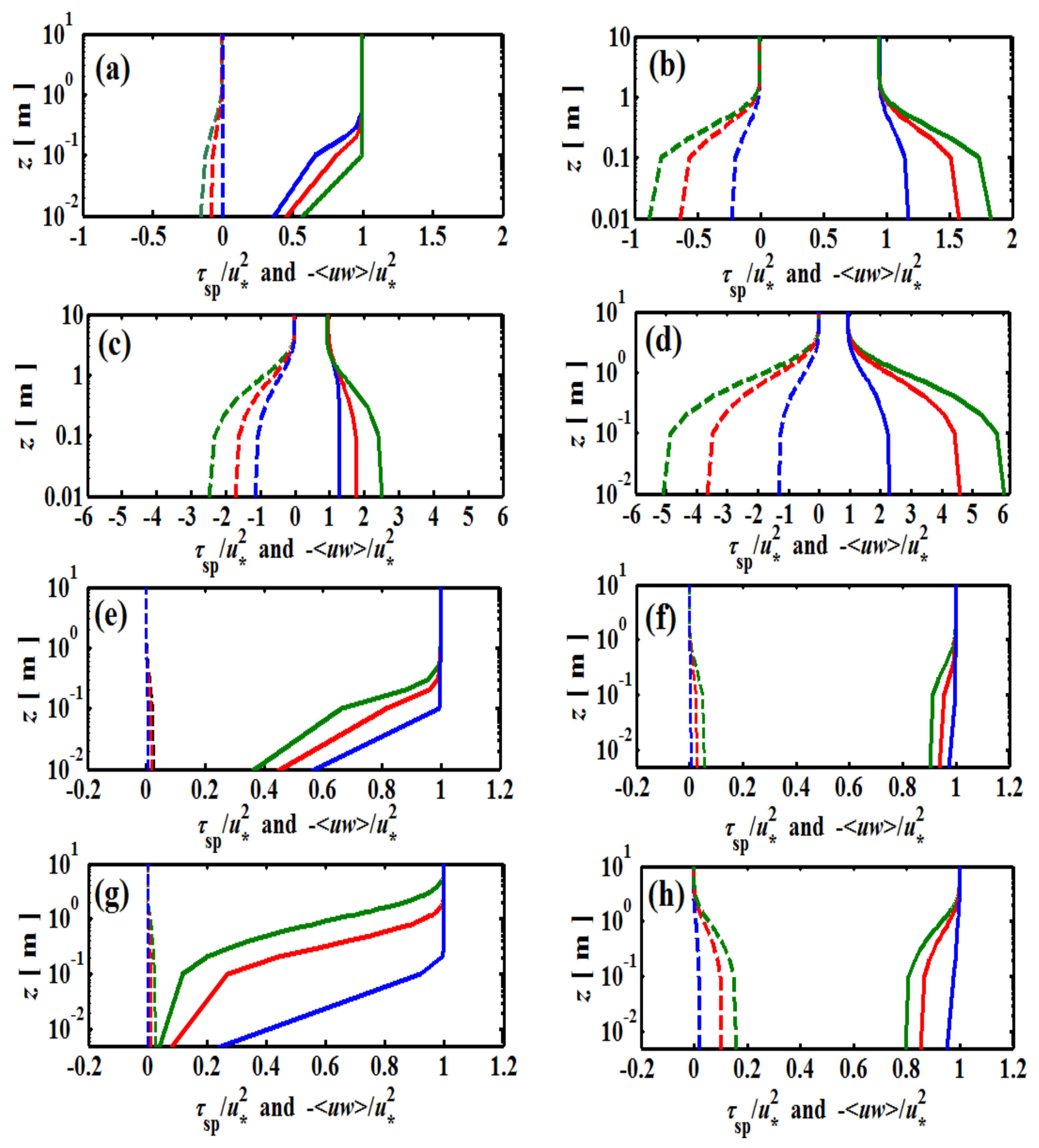
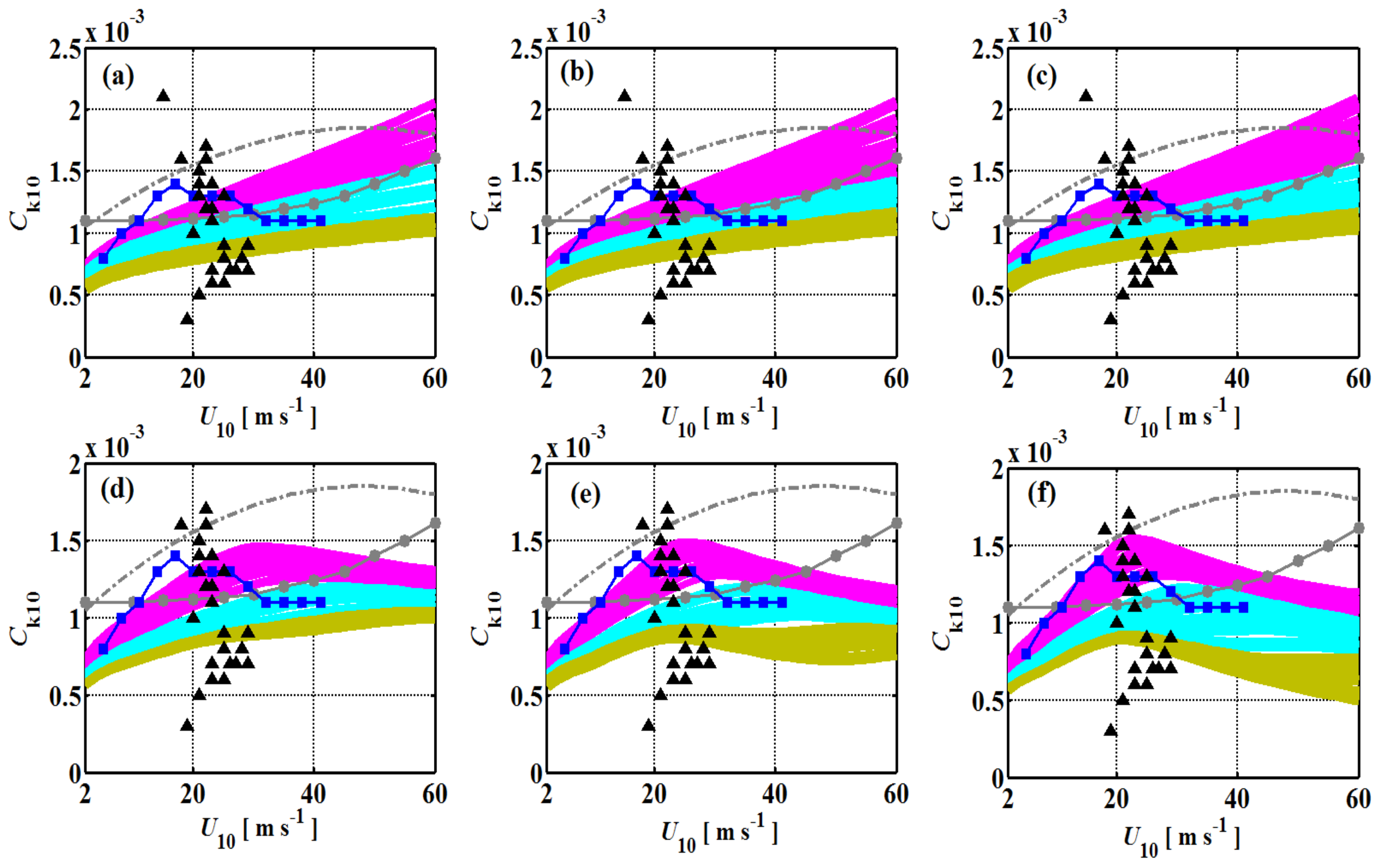
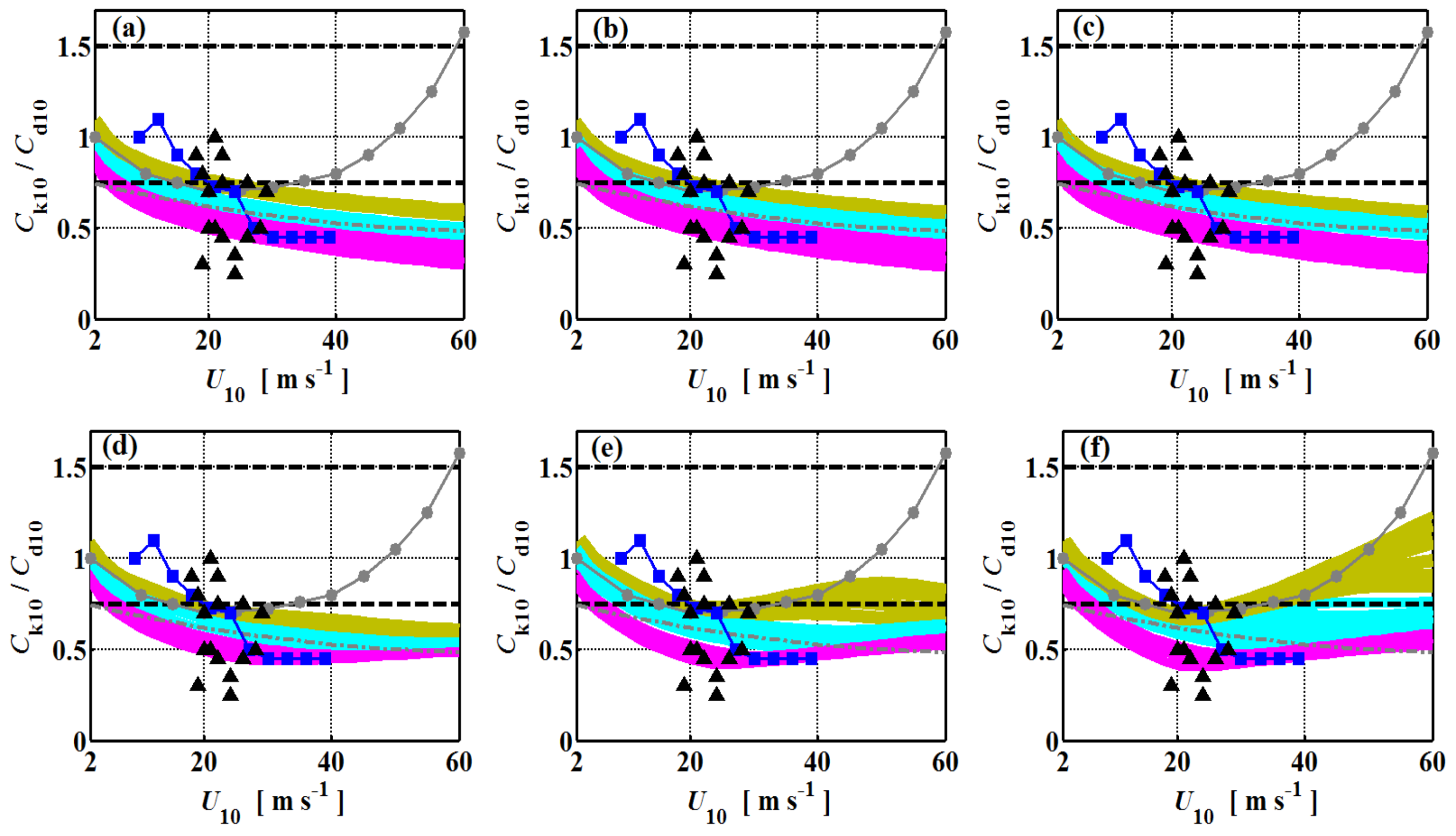
3.1. Momentum Fluxes in the MASL

According to the 12 experiments in Table 1, the model in Section 2.3 is computed, and the non-dimensional turbulent and spray-induced fluxes are shown in Figure 4. The subplots in Figure 4a–d were calculated for $U_{\mathrm{inj}}\left(z\right)=U\left(z\right)$ and those in Figure 4e–h for $U_{\mathrm{inj}}\left(z\right)=\langle U_{\mathrm{b}}\rangle$.

The comparison of Figure 4a and Figure 4c (or Figure 4b and Figure 4d) indicates the turbulent momentum near the sea surface increases with 10 m wind speed. The turbulent momentum fluxes also increase with wave ages (see Figure 4a–d). The magnitude of spray-induced momentum fluxes near the sea surface in Figure 4a–d also increased in absolute value with $U_{10}$ and $\mathsf{\Omega }$, and the negative sign of ${\tau }_{\mathrm{SP}}$ signifies that the accumulation of the three terms on the right side of Equation (15) leads to a negative value. The negative spray-induced momentum fluxes indicate that the momentum transfers from spray droplets into the near-surface airflow in the condition of $U_{\mathrm{inj}}\left(z\right)=U\left(z\right)$. It is interesting to see that the non-dimensional turbulent momentum fluxes in Figure 4b–d decrease with height, whereas those in Figure 4a increase with height. Obviously, in the second case, this result signifies that the turbulent momentum fluxes near the sea surface are lower than those at 10 m when the ratio parameter is set to 0.95 (see Figure 4a). It also reveals that more momentum fluxes are supported by surface waves rather than the airflow when $U_{10}$ is 30 m s⁻¹. When the 10 m wind speed strengthens to 50 m s⁻¹ (see Figure 4c), more momentum is transferred from spray to airflow to enhance the turbulence, although the ratio parameter is as great as 0.95. The comparison of Figure 4b and 4d signifies that the magnitude of the non-dimensional spray-induced momentum fluxes proportionally depends on $U_{10}$ and $\mathsf{\Omega }$. This is attributed to the generation of more spray under high winds and mature wave fields (seen in Figure 2). In addition, the comparison of Figure 2a and Figure 2b (or Figure 2c and Figure 2d) reveals that non-dimensional turbulent momentum fluxes are inversely proportional to ratio parameter $x$. This could be explained by Equation (14), i.e., $-\langle uw\rangle /u_{*}^2+{\tau }_{\mathrm{SP}}/u_{*}^2+x=1$. Then, the increase in $x$ means that the other two terms decline ($-\langle uw\rangle /u_{*}^2$ and ${\tau }_{\mathrm{SP}}/u_{*}^2$) to balance the momentum in the MASL.

When the injection velocity is adopted as $U_{\mathrm{inj}}=\langle U_{\mathrm{b}}\rangle$, Figure 4e–h shows that turbulent momentum near the sea surface decreases with 10 m wind speed and wave ages. The magnitude of spray-induced momentum fluxes near the sea surface in Figure 4a–d also increased with $U_{10}$ and $\mathsf{\Omega }$, and the positive sign of ${\tau }_{\mathrm{SP}}$ signifies that the accumulation of three terms on the right side of Equation (15) leads to a positive value. The positive spray-induced momentum fluxes indicate the momentum transfer from near-surface airflow into spray droplets in the condition of $U_{\mathrm{inj}}\left(z\right)=U\left(z\right)$. It is noticeable in Figure 4e–h that the non-dimensional turbulent momentum fluxes are lower than one near the sea surface and tend to be one with height. This explicitly indicates that the turbulent momentum fluxes at the lower height are smaller than those at 10 m. In addition, the comparison of Figure 4b and Figure 4d signifies that the magnitude of the non-dimensional spray-induced momentum fluxes disproportionately depends on $U_{10}$ and $\mathsf{\Omega }$. This is attributed to the generation of more spray droplets under high winds and mature wave fields so that spray supports more momentum fluxes near the sea surface. The explanation of the impact of the ratio parameter $x$ on the turbulent momentum fluxes in Figure 4e–h also refers to the balance equation, Equation (14). A greater $x$ indicates that more momentum is supported by surface waves so that less momentum is distributed in airflow and spray droplets. Note that the simulation results in this case (see Figure 4e–h) are opposite to those in Figure 4a–d. Therefore, it can be concluded that the injection velocity of spray droplets significantly affects the vertical momentum distribution in the MASL.

To further explore the variations in the drag coefficients $C_{\mathrm{d}10}$ in different conditions, the numerical experiments outlined in Table 2 were conducted based on the MASL models in Section 2.1 and 2.3. Figure 5 shows the simulation results and the available measurements for validation [10,11,12,13]. The dash–dotted line calculated based on the traditional MOST (i.e., COARE 3.5) rapidly increases with wind speeds and deviates from the measurements for $U_{10}$ exceeding 30 m s⁻¹. This signifies that the traditional method fails to evaluate the drag coefficients in high winds. The solid lines in Figure 5a–c were computed based on the MASL in Section 2.1, which considers the spray impact on the TKE balance. The trends of the simulation results agree well with the measurements that $C_{\mathrm{d}10}$ begins to decrease for $U_{10}$ > 30 m s⁻¹. However, the simulated drag coefficients are obviously lower, especially for larger wave ages.

The solid lines in the second and third rows of Figure 5 are calculated based on the MASL model in Section 2.3. Figure 5d–f shows the simulated results for the injection velocity that satisfies $U_{\mathrm{inj}}\left(z\right)=\langle {\mathrm{U}}_{\mathrm{b}}\rangle$. The drag coefficients continuously increase with 10 m wind speeds, which surpass all measurements. Figure 5g–i shows the simulated results for $U_{\mathrm{inj}}\left(z\right)=U\left(z\right)$. It was found that there is a flattening of and then a reduction in $C_{\mathrm{d}10}$ when wind speeds increase to 10 m, which is in accordance with the majority of measurements. These phenomena apparently demonstrate that the injection velocity of spray droplets affects air–sea drag coefficients in high winds. The results in Figure 4 could interpret the difference that exists in Figure 5d–f and Figure 5g–i. In Figure 4b–d, a near-surface $-\langle uw\rangle /u_{*}^2$ greater than 1.0 indicates that the turbulent momentum fluxes near the sea surface are greater than those at 10 m. The larger near-surface turbulent momentum fluxes inhibit the momentum at 10 m to transfer downward so that the 10 m drag coefficients $C_{\mathrm{d}10}$ decrease or level off at high winds (see Figure 5g–i). A similar phenomenon and explanation were also proposed in a previous study [33]. In Figure 4e–h, a near-surface $-\langle uw\rangle /u_{*}^2$ lower than 1.0 implies that the turbulent momentum fluxes near the sea surface are lower than those at 10 m. The lower near-surface turbulent momentum fluxes promote the momentum at 10 m to transfer downward so that the 10 m drag coefficients $C_{\mathrm{d}10}$ constantly increase at strong winds (see Figure 5d–f).

As the ratio parameter $x$ is set as $0.75\le x\le 0.95$, the values of $C_{\mathrm{d}10}$ in Figure 5e–h arrive at the maximum when $U_{10}$ is in the range of 20–50 m s⁻¹. In this situation, the maximum value of $C_{\mathrm{d}10}$ was about 0.0026 for all wave ages. That is to say that the impact of wave ages on the drag coefficients is slight in this range of ratio. This could be explained in terms of Figure 4 as well. The small differences among the solid lines in Figure 4a and Figure 4c signify that wave ages have little influence on the turbulent momentum fluxes when surface waves support the majority of the momentum.

3.2. Enthalpy Fluxes in the MASL

According to the experiment design in Table 2, the simulation results of enthalpy exchange coefficients $C_{\mathrm{k}10}$ are computed based on the MASL model in Section 2.3. The sea surface temperature $T_{\mathrm{s}}$ is set at 298 K, and the air temperature at 10 m above the mean sea surface is set at 296 K. The difference between the moisture at the sea surface and 10 m is set to zero.

The solid lines in Figure 6 illustrate the simulated $C_{\mathrm{k}10}$ in various conditions. For $U_{\mathrm{inj}}=\langle U_{\mathrm{b}}\rangle$, the values of simulated $C_{\mathrm{k}10}$ increase with wind speeds for all wave ages (see Figure 6a–c). Figure 6d–f shows that simulated $C_{\mathrm{k}10}$ stops increasing at high wind speeds for $U_{\mathrm{inj}}\left(z\right)=U\left(z\right)$, which is in accordance with the laboratory and field measurements [40]. Similar behavior between the simulated results in Figure 6a–f and Figure 5d–i indicates that there is a positive correlation between the momentum and heat fluxes. Owing to the rate of drag and enthalpy coefficients providing a maximum estimation of the potential intensity of a tropical cyclone, the ratio $C_{\mathrm{k}10}/C_{\mathrm{d}10}$, varying with $U_{10}$, is shown in Figure 7. The dashed lines in the figure are the theoretical supposition [41], which provides a standard to model tropical cyclones. The rate within 0.75–1.2 is generally used to validate the practicability of their theoretical model [29,42]. When $U_{\mathrm{inj}}=\langle U_{\mathrm{b}}\rangle$ is adopted, the simulated rates for all wave ages and ratio parameters decrease with wind speeds and are lower than 0.75 for 10 m wind speeds stronger than 30 ms⁻¹ (see Figure 7a–c). When the other assumption $U_{\mathrm{inj}}\left(z\right)=U\left(z\right)$ is used, the simulated rates $C_{\mathrm{k}10}/C_{\mathrm{d}10}$ in Figure 7d–f are almost lower than 0.75, except in the condition where the wave age is greater than 0.6 and the ratio parameter $x$ is within 0.05–0.45. In addition, based on the laboratory and field measurements [43], it is proposed that the range of the rate $C_{\mathrm{k}10}/C_{\mathrm{d}10}$ in high winds could be lower than previously thought [29,42]. As shown in Figure 7a–f, this range was covered by the simulated results when the ratio parameter $x$ was within 0.75–0.95. This indicates that the non-breaking surface waves containing a lot of kinetic energy favor the intensification of tropical cyclones. Conclusively, Figure 7 reveals that the spray injection velocity, wave ages, and air–sea fluxes play a crucial role in tropical cyclones.

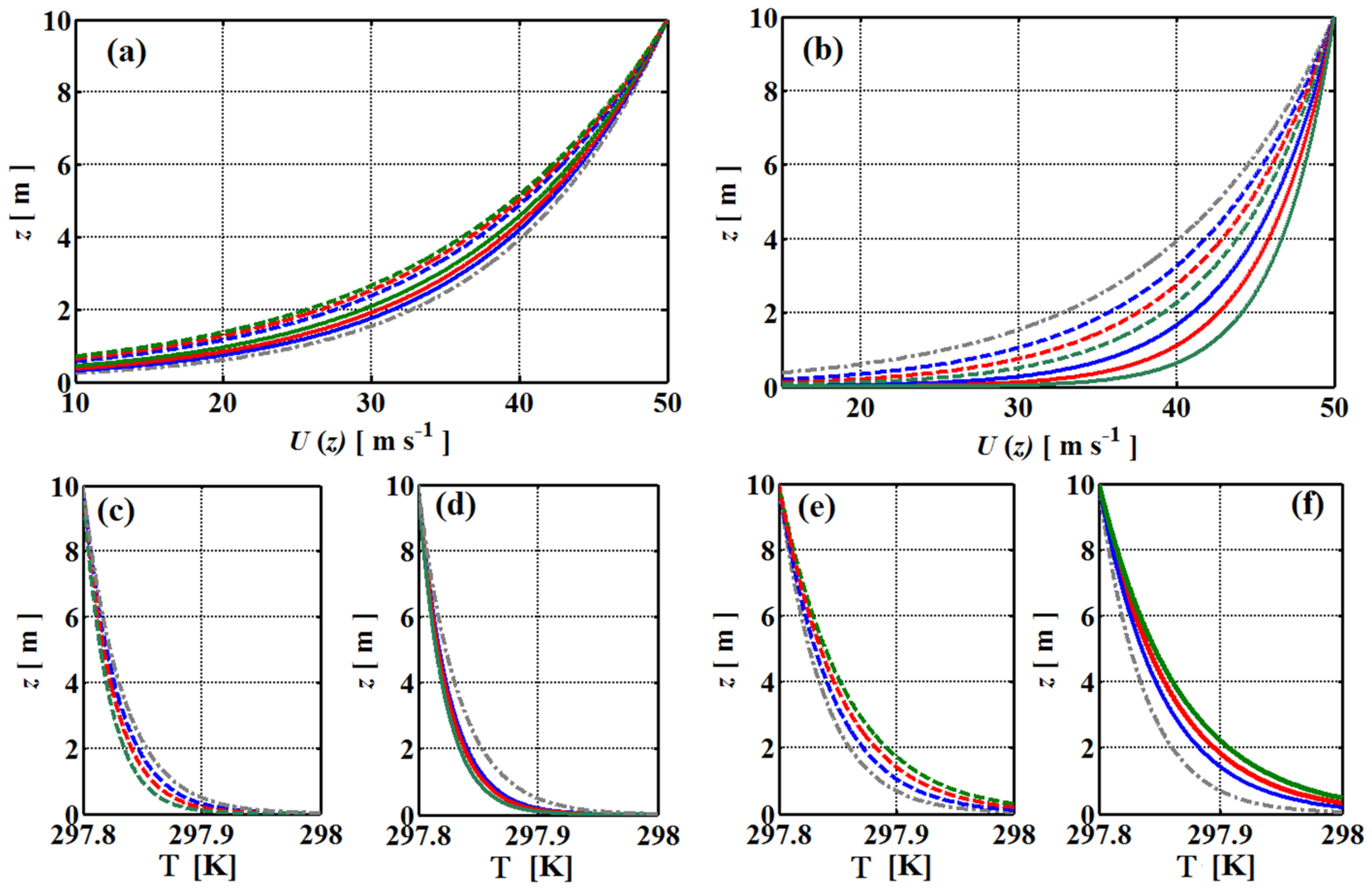
3.3. Vertical Profiles of Mean Wind Speeds and Temperature

According to the MASL model in Section 2.3, the vertical profiles of mean wind speeds are computed for $U_{10}=$ 50 m s⁻¹. The simulated profiles for $U_{\mathrm{inj}}\left(z\right)=\langle U_{\mathrm{b}}\rangle$ and $U_{\mathrm{inj}}\left(z\right)=U\left(z\right)$ are shown in Figure 8. As a comparison, the profiles calculated based on the COARE 3.5 are also illustrated in the figure to present the spray-wave-free case.

For $U_{\mathrm{inj}}\left(z\right)=\langle U_{\mathrm{b}}\rangle$, simulated wind speeds are lower than those in the spray-wave-free condition (see Figure 8a). As discussed in Section 3.1, momentum is transferred from the airflow to waves and spray in this situation. This direction of momentum transfer correspondingly decelerates winds near the sea surface. Because more momentum is transferred from airflow for greater wave ages $\mathsf{\Omega }$ or ratio parameters $x$, the near-surface wind speeds decrease with $\mathsf{\Omega }$ or $x$ at a given height (see Figure 8a).

When $U_{\mathrm{inj}}\left(z\right)=U\left(z\right)$ is assumed, simulated wind profiles are shown in Figure 8b. Opposite to the results in Figure 8a, the impact of waves and spray accelerates the near-surface winds compared to the spray-wave-free case. This phenomenon could also be interpreted based on the momentum distribution in Section 3.1. In this case, about $U_{\mathrm{inj}}\left(z\right)$ momentum is transferred from falling spray droplets to the near-surface airflow. This direction of momentum transfer makes the near-surface winds accelerate correspondingly. At a given height, it is also seen in Figure 8b that wind speeds increase with $x$. This could be interpreted through a comparison of Figure 4c and Figure 4d. When surface waves support a majority of momentum fluxes (i.e., $x=0.95$), the turbulent momentum is relatively low and results in low wind speed.

The simulated profiles of mean temperature are shown in Figure 8c–f. Compared to the spray-wave-free profile, the simulated temperature is lower for $U_{\mathrm{inj}}\left(z\right)=\langle U_{\mathrm{b}}\rangle$, whereas it is greater for $U_{\mathrm{inj}}\left(z\right)=U\left(z\right)$. According to the wind profiles in Figure 8a–b, the behavior of temperature in Figure 8c–f could also be explained. The gradients of wind speeds in Figure 8a decrease compared to the spray-wave-free gradient. This inhibits the sea surface heat from transferring upward so that the air temperature is lower in the MASL (see Figure 8c,d). On the other hand, the gradients of wind speeds in Figure 8b increase compared to the spray-wave-free gradient. This promotes the sea surface heat to transfer upward, which leads to a rise in air temperature in the MASL (see Figure 8e–f). In addition, the temperature decreases with wave ages for $x=0.95$ and is not sensitive to wave ages for $x=0.05$. For $U_{\mathrm{inj}}\left(z\right)=U\left(z\right)$, the simulated temperature is greater than that in the spray-wave-free case (see Figure 6e–f). The temperature increases with wave ages for both values of the ratio parameter $x$.

4. Discussion

Based on the previous spray-laden MOST, this study introduces the effects of spray and waves through coupling spray-laden momentum and enthalpy conservation equations. In the two cases of spray injection velocities, numerical experiments were conducted based on the MASL models to investigate the variation in air–sea fluxes and near-surface wind/temperature profiles. One case assumes that spray droplets are simultaneously accelerated to the velocity of their ambient airflow once injected. Case two treats the spray injection velocity as the same as that of the edges of water bags. The major findings of this study are presented below.

The spray injection velocity plays a significant role in air–sea fluxes and wind/temperature profiles in high winds. On the assumption that the injection velocity equals the ambient wind speed, the simulated results show that the sign of the spray-induced momentum is negative, which indicates that the momentum is transferred from the spray to near-surface airflow. This gain in the momentum to the airflow makes the near-surface momentum fluxes increase so that the momentum at 10 m of the MASL is inhibited. Therefore, 10 m drag end enthalpy exchange coefficients decrease at strong winds. The near-surface wind speed and temperature also increase due to the enhancement of the turbulence. Based on the other assumption that the injection velocity is approximated by the velocity of the edges of water bags, the simulated results indicate that the sign of the spray-induced momentum is positive. This signifies that the momentum transfers from near-surface airflow to spray droplets, which makes the near-surface momentum fluxes decrease and promotes the momentum at 10 m to transfer downward. Therefore, the 10 m drag and enthalpy exchange coefficients increase at high winds. Near-surface wind speed and temperature also decrease due to the reduction in the near-surface turbulent momentum.

The simulated results also show that surface waves affect air–sea fluxes and wind/temperature profiles in two ways, i.e., wave ages and wave-induced momentum fluxes. Since the spray concentration has a positive correlation to wave ages, the impact of spray on the near-surface turbulent momentum fluxes increases with wave ages. When non-breaking waves support the majority of the momentum, spray-induced momentum fluxes tend to be small to balance the momentum. In this situation, the impact of spray on the turbulent momentum flux is small.

In order to consider a few observations to provide a physical analysis of air–sea fluxes, this study used the model in Section 2 and some control experiments in Section 3 to provide a theoretical explanation of how spray and waves affect the MASL. This will hopefully inspire people to further explore small-scale air–sea processes within extreme ocean conditions. The factors that affect the MASL are not limited to ocean waves and spray. Other phenomena, such as foam, breaking waves, and white caps, also play an important role in air–sea interactions in high winds. Observations showed that white caps that were the patches of active foam created by breaking waves made the sea surface smoother for surface wind speeds larger than 40 m s⁻¹ [12]. To a certain extent, this indicates that the white cap could suppress the exchange of the air–sea momentum. Laboratory and satellite measurements also revealed that the fraction of foam coverage effectively influenced wind–wave interaction [44,45]. Nevertheless, this mechanism is not considered in this study. Obtaining observational data to parameterize the fraction foam coverage is another challenging task [46,47]. In future research, the relationship between the energy dissipation rate of breaking waves and white cap coverage should be included in the MASL model [48,49].

References

1. Song, J.B.; Huang, Y.S. An approximate solution of wave-modified Ekman current for gradually varying eddy viscosity. Deep Sea Res. Part I Oceanogr. Res. Pap. 2011, 58, 668–676. [Google Scholar] [CrossRef]
2. Hell, M.C.; Ayet, A.; Chapron, B. Swell generation under extra-tropical storms. J. Geophy. Res. Oceans 2021, 126, e2021JC017637. [Google Scholar] [CrossRef]
3. Voermans, J.J.; Rapizo, H.; Ma, H.Y.; Qiao, F.L.; Babanin, A.V. Air-sea momentum fluxes during cyclone olwyn. J. Phys. Oceanogr. 2019, 49, 1369–1379. [Google Scholar] [CrossRef]
4. Wu, L.C.; Rutgersson, A.; Sahle, E.; Larsen, X.G. The impact of waves and sea spray on modelling storm track and development. Tellus A Dyn. Meteorol. Oceanogr. 2015, 67, 27967. [Google Scholar] [CrossRef]
5. Chen, Y.J.; Yu, X. Enhancement of wind stress evaluation method under storm conditions. Clim. Dyn. 2016, 47, 3833–3843. [Google Scholar] [CrossRef]
6. Zhang, T.; Song, J.B.; Li, S.; Yang, L.G. The effects of wind-driven waves and ocean spray on the drag coefficient and near-surface wind profiles over the ocean. Acta Ocean. Sin. 2016, 35, 79–85. [Google Scholar] [CrossRef]
7. Zhang, T.; Song, J.B. Effects of sea-surface waves and ocean spray on air-sea momentum fluxes. Adv. Atmos. Sci. 2018, 35, 469–478. [Google Scholar] [CrossRef]
8. Veron, F. Ocean spray. Ann. Rev. Flu. Mech. 2015, 47, 507–538. [Google Scholar] [CrossRef]
9. Alamaro, M.; Emanuel, K.; Colton, J.; McGillis, W.; Edson, J. Experimental investigation of air-sea transfer of momentum and enthalpy at high wind speed. In Preprints, Proceedings of the 25th Conference on Hurricanes and Tropical Meteorology, San Diego, CA, USA, 29 April 2002; American Meteorological Society: Boston, MA, USA, 2002; pp. 667–668. [Google Scholar]
10. Powell, M.D.; Vickery, P.J.; Reinhold, T.A. Reduced drag coefficient for high wind speeds in tropical cyclones. Nature 2003, 422, 279. [Google Scholar] [CrossRef]
11. Jarosz, E.; Mitchell, D.A.; Wang, D.W.; Teague, W.J. Bottom-up determination of air-sea momentum exchange under a major tropical cyclone. Science 2007, 315, 1707–1709. [Google Scholar] [CrossRef]
12. Holthuijsen, L.H.; Powell, M.D.; Pietrzak, J.D. Wind and waves in extreme hurricanes. J. Geophys. Res. Oceans 2012, 117. [Google Scholar] [CrossRef]
13. Donelan, M.; Haus, B.; Reul, N.; Plant, W.; Stiassnie, M.; Graber, H.; Brown, O.; Saltzman, E. On the limiting aerodynamic roughness of the ocean in very strong winds. Geophys. Res. Lett. 2004, 31. [Google Scholar] [CrossRef]
14. Black, P.G.; D’Asaro, E.A.; Drennan, W.M.; French, J.R.; Niiler, P.P.; Sanford, T.B.; Terrill, E.J.; Walsh, E.J.; Zhang, J.A. Air–Sea Exchange in Hurricanes: Synthesis of Observations from the Coupled Boundary Layer Air–Sea Transfer Experiment. Bull. Am. Meteorol. Soc. 2007, 88, 357–374. [Google Scholar] [CrossRef]
15. Curcic, M.; Haus, B.K. Revised estimates of ocean surface drag in strong winds. Geophys. Res. Lett. 2020, 47, e2020GL087647. [Google Scholar] [CrossRef]
16. Liu, B.; Guan, C.; Xie, L. The wave state and sea spray related parameterization of wind stress applicable from low to extreme winds. J. Geophys. Res. Oceans 2012, 117. [Google Scholar] [CrossRef]
17. Shi, J.; Zhong, Z.; Li, X.; Jiang, G.; Zeng, W.; Li, Y. The influence of wave state and sea spray on drag coefficient from low to high wind speeds. J. Ocean Univ. China 2016, 15, 41–49. [Google Scholar] [CrossRef]
18. Sroka, S.; Emanuel, K. A review of parameterizations for enthalpy and momentum fluxes from sea spray in tropical cyclones. J. Phys. Oceanogr. 2021, 51, 3053–3069. [Google Scholar] [CrossRef]
19. Shpund, J.; Pinksy, M.; Khain, A. Microphysical structure of the marine boundary layer under strong wind and spray formation as seen from simulations using a 2D explicit microphysical model. Part I: The impact of large eddies. J. Atmos. Sci. 2011, 68, 2366–2384. [Google Scholar] [CrossRef]
20. Shpund, J.; Zhang, J.; Pinsky, M.; Khain, A. Microphysical structure of the marine boundary layer under strong wind and spray formation as seen from simulations using a 2D explicit microphysical model. Part II: The role of sea spray. J. Atmos. Sci. 2012, 69, 3501–3514. [Google Scholar] [CrossRef]
21. Shpund, J.; Zhang, J.; Pinsky, M.; Khain, A. Microphysical structure of the marine boundary layer under strong wind and sea spray formation as seen from a 2D explicit microphysical mode. Part III: Parameterization of height-dependent droplet size distribution. J. Atmos. Sci. 2014, 71, 1914–1934. [Google Scholar] [CrossRef]
22. Bianco, L.; Bao, J.W.; Fairall, C.; Michelson, S. Impact of sea-spray on the atmospheric surface layer. Bound. Layer Meteorol. 2011, 140, 361. [Google Scholar] [CrossRef]
23. Rastigejev, Y.; Suslov, S.A. Effect of evaporating sea spray on heat fluxes in a marine atmospheric boundary layer. J. Phys. Oceanogr. 2019, 49, 1927–1948. [Google Scholar] [CrossRef]
24. Chen, X. How do planetary boundary layer schemes perform in hurricane conditions: A comparison with large-eddy simulations. J. Adv. Model. Earth Sys. 2022, 14, e2022MS003088. [Google Scholar] [CrossRef]
25. Li, M.; Zhang, J.A.; Matak, L.; Momen, M. The impact of adjusting momentum roughness length on strong and weak Hurricane Forecasts: A comprehensive analysis of weather simulations and observations. Mon. Wea. Rev. 2023, 151, 1287–1302. [Google Scholar] [CrossRef]
26. Troitskaya, Y.; Ezhova, E.; Soustova, I.; Zilitinkevich, S.S. On the effect of sea spray on the aerodynamic surface drag under sever winds. Ocean Dyn. 2016, 66, 659–669. [Google Scholar] [CrossRef]
27. Druzhinin, O.A.; Troitskaya, Y.I.; Zilitinkevich, S.S. The study of droplet-laden turbulent airflow over waved water surface by direct numerical simulation. J. Geophys. Res. Oceans 2017, 122, 1789–1807. [Google Scholar] [CrossRef]
28. Druzhini, O.A.; Troitskaya, Y.I.; Zilitinkevich, S.S. The study of momentum, mass and heat transfer in a droplet-laden turbulent airflow over a waved-water surface by direct numerical simulation. J. Geophys. Res. Oceans 2018, 123, 8346–8365. [Google Scholar] [CrossRef]
29. Bao, J.W.; Fairall, C.W.; Michelson, S.; Bianco, L. Parameterizations of sea-spray impact on the air-sea momentum and heat fluxes. Mon. Wea. Rev. 2011, 139, 3781–3797. [Google Scholar] [CrossRef]
30. Troitskaya, Y.; Kandaurov, A.; Ermakova, O.; Kozlov, D.; Sergee, D.; Zilitinkevich, S. The “bag breakup” spume droplet generation mechanism at high winds. Part I: Spray generation function. J. Phys. Oceanogr. 2018, 48, 2167–2188. [Google Scholar] [CrossRef]
31. Högström, U.L.F. Non-dimensional wind and temperature profiles in the atmospheric surface layer: A re-evaluation. Top. Micrometeorol. A Festschr. Arch Dye. 1988, 42, 55–78. [Google Scholar]
32. Foken, T. 50 years of the Monin–Obukhov similarity theory. Bound. Layer Meteorol. 2006, 119, 431–447. [Google Scholar] [CrossRef]
33. Kudryavtsev, V.N.; Makin, V.K. Impact of ocean spray on the dynamics of the marine atmospheric boundary layer. Bound. Layer Meteorol. 2011, 140, 383–410. [Google Scholar] [CrossRef]
34. Troitskaya, T.; Druzhinin, O.; Kozlov, D.; Zilitinkevich, S. The “bag breakup” spume droplet generation mechanism at high winds. Part II: Contribution to momentum and enthalpy transfper. J. Phys. Oceanogr. 2018, 48, 2189–2207. [Google Scholar] [CrossRef]
35. Janssen, P.A. Quasi-linear theory of wind-wave generation applied to wave forecasting. J. Phys. Oceanogr. 1991, 21, 1631–1642. [Google Scholar] [CrossRef]
36. Ortiz-Suslow, D.G.; Haus, B.K.; Mehta, S.; Laxague, N.J. Sea spray generation in very high winds. J. Atmos. Sci. 2016, 73, 3975–3995. [Google Scholar] [CrossRef]
37. Veron, F.; Hopkins, C.; Harrison, E.; Mueller, J. Sea spray spume droplet production in high wind speeds. Geophys. Res. Lett. 2012, 39. [Google Scholar] [CrossRef]
38. Fairall, C.; Banner, M.; Peirson, W.; Asher, W.; Morison, R. Investigation of the physical scaling of sea spray spume droplet production. J. Geophys. Res. Oceans 2009, 114. [Google Scholar] [CrossRef]
39. Edson, J.B.; Jampana, V.; Weller, R.A.; Bigorre, S.P.; Plueddemann, A.J.; Fairall, C.W.; Miller, S.D.; Mahrt, L.; Vickers, D.; Hersbach, H. On the exchange of momentum over the open ocean. J. Phys. Oceanogr. 2013, 43, 1589–1610. [Google Scholar] [CrossRef]
40. Hara, T.; Sullivan, P.P. Wave boundary layer turbulence over surface waves in a strongly forced condition. J. Phys. Oceanogr. 2015, 45, 868–883. [Google Scholar] [CrossRef]
41. Emanuel, K.A. Sensitivity of tropical cyclones to surface exchange coefficients and a revised steady-state model incorporating eye dynamics. J. Atmos. Sci. 1995, 52, 3969–3976. [Google Scholar] [CrossRef]
42. Zweers, N.; Makin, V.; Vries, J.; Kudryavtsev, V. The impact of spray-mediated enhanced enthalpy and reduced drag coefficients in the modelling of tropical cyclones. Bound. Layer Meteorol. 2015, 155, 501–514. [Google Scholar] [CrossRef]
43. Haus, B.K.; Jeong, D.; Donelan, M.A.; Zhang, J.A.; Savelyev, I. Relative rates of sea-air heat transfer and frictional drag in very high winds. Geophys. Res. Lett. 2010, 37. [Google Scholar] [CrossRef]
44. Troitskaya, Y.; Sergeev, D.; Kandaurov, A.; Vdovin, M.; Zilitinkevich, S. The effect of foam on waves and the aerodynamic roughness of the water surface at high winds. J. Phys. Oceanogr. 2019, 49, 959–981. [Google Scholar] [CrossRef]
45. Reul, N.; Chapron, B. A model of sea-foam thickness distribution for passive microwave remote sensing applications. J. Geophy. Res. Oceans 2003, 108. [Google Scholar] [CrossRef]
46. Golbraikh, E.; Shtemler, Y.M. Foam input into the drag coefficient in hurricane conditions. Dyn. Atmos. Oceans 2016, 73, 1–9. [Google Scholar] [CrossRef]
47. Hwang, P.A.; Reul, N.; Meissner, T.; Yueh, S. Whitecap and wind stress observations by microwave radiometers: Global coverage and extreme conditions. J. Phys. Oceanogr. 2019, 49, 2291–2307. [Google Scholar] [CrossRef]
48. Callaghan, A.H. On the relationship between the energy dissipation rate of surface-breaking waves and oceanic whitecap coverage. J. Phys. Oceanogr. 2018, 48, 2609–2626. [Google Scholar] [CrossRef]
49. Xie, Z. Numerical modelling of wind effects on breaking waves in the surf zone. Ocean Dyn. 2017, 67, 1251–1261. [Google Scholar] [CrossRef]
Figure 1. Sketch of the spray-laden MASL at high winds. Solid wavy lines denote the non-breaking waves propagating in the x direction. The circles denote the suspended spray droplets.
Atmosphere 14 01500 g001
Figure 2. (a) Comparison of d F r / d r in Equation (28) with others. The solid lines correspond to U 10 = 30 m s−1 (blue), 40 m s−1 (red), and 50 m s−1 (black) for Ω = 1.0; the dashed lines correspond to U 10 = 30 m s−1 (blue), 40 m s−1 (red), and 50 m s−1 (black) for Ω = 0.1. Symbols linked by dotted lines are measurements and described as follows: squares for U 10 = 36 m s−1, 45 m s−1, and 49.5 m s−1 [36]; circles for U 10 = 41.5 m s−1 and 47.1 m s−1 [37]; and diamonds for u * = 1.44 m s−1 and 1.64 m s−1 [38]. (b) Comparison of SSGF in Equation (28) as the volume flux with previous theoretical results [33]. The solid lines correspond to U 10 = 30 m s−1 (green), 40 m s−1 (red), and 50 m s−1 (orange) for Ω = 1.0; the dashed lines correspond to U 10 = 30 m s−1 (green), 40 m s−1 (red), and 50 m s−1 (orange) for Ω = 0.1. The dash–dotted lines were previously theoretical for u * = 1.35 m s−1, 1.44 m s−1 (red), and 1.64 m s−1 (yellow) [33].
Atmosphere 14 01500 g002
Figure 3. Vertical profiles of the spray volume flux F S z . The solid lines correspond to U 10 = 30 m s−1 (blue), 40 m s−1 (red), and 50 m s−1 (black) for Ω = 1.0; the dashed lines correspond to U 10 = 30 m s−1 (blue), 40 m s−1 (red), and 50 m s−1 (black) for Ω = 0.1.
Atmosphere 14 01500 g003
Figure 4. Vertical profiles of non-dimensional spray-induced and turbulent momentum fluxes, i.e., τ SP / u * 2 (dashed lines) and u w / u * 2 (solid lines). Subplots (ad) for U inj z = U z , and subplots (eh) for U inj z = U b . The 10 m wind speeds are set at U 10 = 30 m s−1 in subplots (a,b,e,f) and U 10 = 50 m s−1 in subplots (c,d,g,h). The ratio parameter x is set at 0.95 in subplots (a,c,e,g) and 0.05 in subplots (b,d,f,h). The colors denote wave ages, i.e., Ω = 0.2 (blue), 0.6 (red), and 1.0 (green).
Atmosphere 14 01500 g004
Figure 5. For three wave-age parameters, i.e., Ω = 0.2 (a,d,g), 0.6 (b,e,h), and 1.0 (c,f,i). Solid lines in subplots (ac) denote C d 10 versus U 10 calculated based on Section 2.1. Solid lines in subplots (di) denote C d 10 versus U 10 calculated based on Section 2.3. Subplots (df) are for U inj z = U b , and subplots (gi) are for U inj z = U z . The colors of the solid lines denote 0.05 x 0.45 (blue), 0.45 x 0.75 (green), and 0.75 x 0.95 (pink). The grey dash–dotted lines resulted from the traditional MOST (i.e., COARE 3.5 [39]). Grey squares and magenta circles are field and laboratory measurements [12,13]. Red and black dashed lines represent the field observations [10,11].
Atmosphere 14 01500 g005
Figure 6. For three wave ages, i.e., Ω = 0.2 (a,d), 0.6 (b,e), and 1.0 (c,f). The solid lines denote 10 m enthalpy exchange coefficients C k 10 . Subplots (ac) are for U inj z = U b , and subplots (df) are for U inj z = U z . The colors of the solid lines denote 0.05 x 0.45 (green), 0.45 x 0.75 (blue), and 0.75 x 0.95 (purple), respectively. The grey dash–dotted lines are calculated based on the traditional MOST (i.e., COARE 3.5) [39]. The circles denote the simulation results based on the MASL model in Section 2.1. The blue squares and black triangles denote laboratory and field measurements, respectively [42].
Atmosphere 14 01500 g006
Figure 7. For three wave ages, i.e., Ω = 0.2 (a,d), 0.6 (b,e), and 1.0 (c,f). The solid lines denote the simulated C k 10 / C d 10 . Subplots (ac) are for U inj z = U b , and subplots (df) are for U inj z = U z . The colors of the solid lines denote 0.05 x 0.45 (green), 0.45 x 0.75 (blue), and 0.75 x 0.95 (purple), respectively. The grey dash–dotted lines are calculated based on the traditional MOST (i.e., COARE 3.5) [39]. The black dashed lines are the theoretical range [41]. The gray circles are the simulated results from Section 2.1. The blue squares and black triangles are laboratory and field measurements [42].
Atmosphere 14 01500 g007
Figure 8. Subplots (a–b) are vertical profiles of mean wind speed for (a) U inj z = U b and (b) U inj z = U z ; dash and solid lines denote wind profiles for x = 0.95 and 0.05 , respectively; colors Ω = 0.2 (blue), 0.6 (red), and 1.0 (green) denote wave ages. Subplots (cf) are vertical profiles of temperature for (c,d) U inj z = U b and (e,f) U inj z = U z . The description of line styles and colors are as same as those in subplots (a,b). The grey dash–dotted line is calculated based on COARE 3.5 [39].
Atmosphere 14 01500 g008