Inversion Method for Multiple Nuclide Source Terms in Nuclear Accidents Based on Deep Learning Fusion Model

Abstract

During severe nuclear accidents, radioactive materials are expected to be released into the atmosphere. Estimating the source term plays a significant role in assessing the consequences of an accident to assist in actioning a proper emergency response. However, it is difficult to obtain information on the source term directly through the instruments in the reactor because of the unpredictable conditions induced by the accident. In this study, a deep learning-based method to estimate the source term with field environmental monitoring data, which utilizes the bagging method to fuse models based on the temporal convolutional network (TCN) and two-dimensional convolutional neural network (2D-CNN), was developed. To reduce the complexity of the model, the particle swarm optimization algorithm was used to optimize the parameters in the fusion model. Seven typical radionuclides (Kr-88, I-131, Te-132, Xe-133, Cs-137, Ba-140, and Ce-144) were set as mixed source terms, and the International Radiological Assessment System was used to generate model training data. The results indicated that the average prediction error of the fusion model for the seven nuclides in the test set was less than 10%, which significantly improved the estimation accuracy compared with the results obtained by TCN or 2D-CNN. Noise analysis revealed the fusion model to be robust, having potential applicability toward more complex nuclear accident scenarios.

1. Introduction

Although the design of nuclear power plants is based on the principle of multi-barriers with relatively good safety preparation, the Fukushima nuclear accident [1] warned that nuclear accidents due to reactor design defects, personnel operation errors, and natural disasters are still possible. After a nuclear accident, it is necessary to quickly estimate the total amount and composition of radionuclides released. Subsequently, the dose distribution in the area around the nuclear accident was simulated based on the estimated source term to support decision makers in taking the most reasonable accident disposal measures [2]. Therefore, estimating the source term is crucial.

There are two methods for source term estimation [3], of which one is to estimate the release source term of a nuclear accident based on the operating conditions of a nuclear plant. The other is to estimate the release source term of a nuclear accident using radioactive environmental monitoring data, which is also known as source term inversion. After severe nuclear accidents, monitoring instruments in nuclear power plants are often damaged [4], which makes it difficult to obtain the operating conditions of nuclear power plants. Therefore, source term inversions have received extensive attention. Because the gamma dose rate in air can be measured rapidly and in real-time, there have been many research methods to estimate source terms based on gamma dose rate monitoring data, including optimal interpolation [5], data assimilation [6,7,8], Kalman filtering [9,10], Bayesian methods [11,12], and least squares [13,14,15,16,17,18]. Since the Fukushima accident, more attentions have been paid to source term inversion and more methods have been used to perform the study [19,20,21]. However, these methods require long-term monitoring of data to ensure that the algorithms converge. A poor initial value can lead to computational failure or slow convergence, thereby requiring reliable a priori information as a basis. The neural network approach eliminates this dilemma. It does not require prior information, and with its powerful self-learning capability, it can identify the corresponding relationship from the gamma dose rate monitoring data and predict the source term based on the corresponding relationship.

In our previous study, we demonstrated that a backpropagation neural network model can effectively predict a single nuclide [22] and classify complex multi-nuclide source terms [23]. Thereafter, a recurrent neural network model was built to obtain the release rates of the six nuclides by sequential processing of the gamma dose rates [24]. The MAPE of the test dataset reached 15.92%, 6.57%, 18.45%, and 36.80% for the nuclides Sr-91, Te-132, Xe-133, and I-131 at the 10th hour, respectively. However, the MAPE remained stable at 67% for La-140 and Cs-137 [24]. To further reduce the prediction error, a temporal convolutional neural network (TCN) model with a strong analysis capability for time series was established [25]. Currently, it is noted that a two-dimensional convolutional neural network (2D-CNN) is capable of extracting deeper features from the original data by transforming the one-dimensional time-series signals into two-dimensional image data using polar coordinates, which greatly improves the prediction accuracy of multiple experiments [26]. In addition, a fusion algorithm that combines several deep-learning models is highly conducive to enhancing the generalization ability, which can assist in method adaptation to a wide variety of data.

In this study, a method for multiple nuclide source term inversion in nuclear accidents based on a deep learning fusion model is proposed. The bagging algorithm was utilized to fuse the TCN and 2D-CNN models to maximize their respective strengths. The weights between them were optimized using the particle swarm algorithm. The gamma dose rate and meteorological conditions were used as combined inputs of the model, and the release rate of the multi-nuclide source term was used as the output of the model. Deep learning-based inversion models for nuclear accident source terms require a large amount of data to train the complex nonlinear relationship between off-site monitoring data and the source term; therefore, it is necessary to obtain a large training dataset. In this study, the International Radiological Assessment System (InterRAS) [27] was used to simulate the atmospheric dispersion of radionuclides and generate the datasets required for the model. The gamma dose rate and meteorological conditions were used as combined inputs of the model, and the release rates of the multi-nuclide (seven typical radionuclides (Kr-88, I-131, Te-132, Xe-133, Cs-137, Ba-140, and Ce-144) were the outputs of the model. Additionally, Bayesian optimization and hyperband (BOHB) can be used to determine the optimal hyperparameters in high-dimensional data space to obtain better performance.

2. Materials and Methods

2.1. Severe Nuclear Accident Model and Dataset Generation

2.1.1. Definition of the Multi-Nuclide Source Term

In this model, it is assumed that seven typical radionuclides—Kr-88, Te-132, I-131, Xe-133, Cs-137, Ba-140, and Ce-144—are released into the environment at constant rates. The duration of the release was set to 30 min. The approximate order-of-magnitude ranges for the release rates of the seven radionuclides were calculated, as shown in

Table 1. Information on the seven radionuclides set as source item.

Nuclide	Half-Life	Activity per MW (1012 Bq/MW)	Atmospheric Immersion Dose Conversion Factor (Sv s−1 per Bq m−3)	Ground Deposition Dose Conversion Factor (Sv s−1 per Bq m−2)	Approximate Order of Magnitude of Release Rate (Bq/h)
Kr-88	2.8 h	830	1.02 × 10−13		1018
Te-132	3.3 d	1400	1.03 × 10−14	2.28 × 10−16	1018
I-131	8.1 d	940	1.82 × 10−14	3.76 × 10−16	1018
Xe-133	5.3 d	1940	1.56 × 10−15		1019
Cs-137	30.1 y	70	7.74 × 10−18	2.85 × 10−19	1017
Ba-140	12.8 d	1800	8.58 × 10−15	1.80 × 10−16	1018
Ce-144	284 d	990	8.53 × 10−16	2.03 × 10−17	1018

. They refer to the calculation results according to a severe nuclear accident with release category PWR1 by referring to the core inventory of a 2905 MW-pressurized water reactor at the end of its lifetime described in the reactor safety study [28]. The detailed calculation process is shown in the Table S1 from Supplementary Materials.

2.1.2. Locations of Monitoring Sites

The two downwind monitoring points were 1 km and 5 km away from the release point, respectively. Gamma dose rates were calculated.

2.1.3. Other Input Data

Other input data include release height, atmospheric stability, wind speed, mixed layer height, and precipitation type. The range of values for these input parameters was set based on historical meteorological data around the coastal nuclear power plant, as shown in

Table 2. Release height and meteorological parameter setting range.

Auxiliary Data	Value Range	Description
Release Height	0–60 m	Release height affects the maximum extent of nuclide dispersion, and wind speed will vary at different heights.
Atmospheric Stability	A–G	Pasquill’s atmospheric stability category, indicating the tendency and degree of the air mass to return to or move away from the original equilibrium position after the air is disturbed in a vertical direction. A–G indicate conditions from an extremely unstable to an extremely stable state.
Wind Speed	0–12 m/s	Wind speed directly affects the diffusion rate of radionuclides.
Mixed Layer Height	100–800 m	Mixed layer height affects the diffusion of nuclides in the vertical direction.
Precipitation Type	None Light Rain (rainfall rate < 25 mm/h) Medium Rain (rainfall rate between 25 and 75 mm/h) Heavy Rain (rainfall rate > 75 mm/h) Light Snow (visibility > 1 km) Middle Snow (visibility between 0.5 and 1 km) Heavy Snow (visibility < 0.5 km)	Precipitation will accelerate deposition of the nuclide.

.

2.1.4. Dataset Generation

Source term data and other input data were randomly generated within the range of values in Table 1 and Table 2. The source term data and other input data were input into InterRAS to calculate the gamma dose rates per hour in 10 h following the release at the two monitoring sites. The meteorological parameters remained unchanged during the 10 h of the simulation. A total of 10,000 sets of data were computed, of which 9000 were used as the training set of the neural network and the remaining 1000 were used as the test set. An example of a dataset is presented in

Table 3. A sample data set.

Source Term		Auxiliary Data		Time (h)	Gamma Dose Rate (mSv/h)
Radionuclide	Release Rate (Bq/h)				1 Km Downwind	5 Km Downwind
88Kr	2.67 × 1018	Release Height (m)	37	1	3240	538
132Te	4.7 × 1018	Wind Speed (m/s)	8	2	3700	620
131I	9.8 × 1018	Mixed Layer Height (m)	457	3	4500	800
133Xe	2.7 × 1019	Atmospheric Stability	C	4	4000	800
137Cs	6.98 × 1017	Precipitation Type	Heavy Snow	5	5000	800
140Ba	7.45 × 1018			6	6000	900
144Ce	3.63 × 1018			7	5000	900
				8	5000	1000
				9	6000	900
				10	6000	1000

.

An in-house script was compiled using Python 3.7.7 and was used to implement the numerous calculations, running on a personal computer with a 32-bit Win7 system.

2.2. Inversion Model Based on TCN

2.2.1. TCN Algorithm

An artificial neural network (ANN) is an algorithmic mathematical model that simulates the structure and behavior of the biological nervous system for distributed parallel information processing with strong robustness, memory capability, and self-learning ability. A convolutional neural network (CNN) is a type of ANN that can analyze small pieces of raw data to obtain deeper data features. A temporal convolutional neural network (TCN) [29] based on a one-dimensional CNN can efficiently process time-sequential data by introducing a causal dilated convolution structure.

To ensure no information “leakage” from the future to the past, the causal convolution structure is used in the TCN model. In this causal convolution structure, the output at time t is convolved only with the input at time t and prior to it. Suppose that we are given input time-sequential data $x_0, x_1, \dots , x_t$ and the corresponding outputs $y_0, y_1, \dots , y_t$, at each time. The causal convolution structure is that to predict the output $y_t$ for some time t, we are constrained to only use those inputs that have been previously observed: $x_0, x_1, \dots , x_t$. Formally, the causal convolution structure is a function $f:X^{t+1}\to Y^{t+1}$ which produces a mapping

$${\widehat{y}}_0,{\widehat{y}}_1, \dots ,{\widehat{y}}_t=f\left(x_0, x_1, \dots , x_t\right)$$

(1)

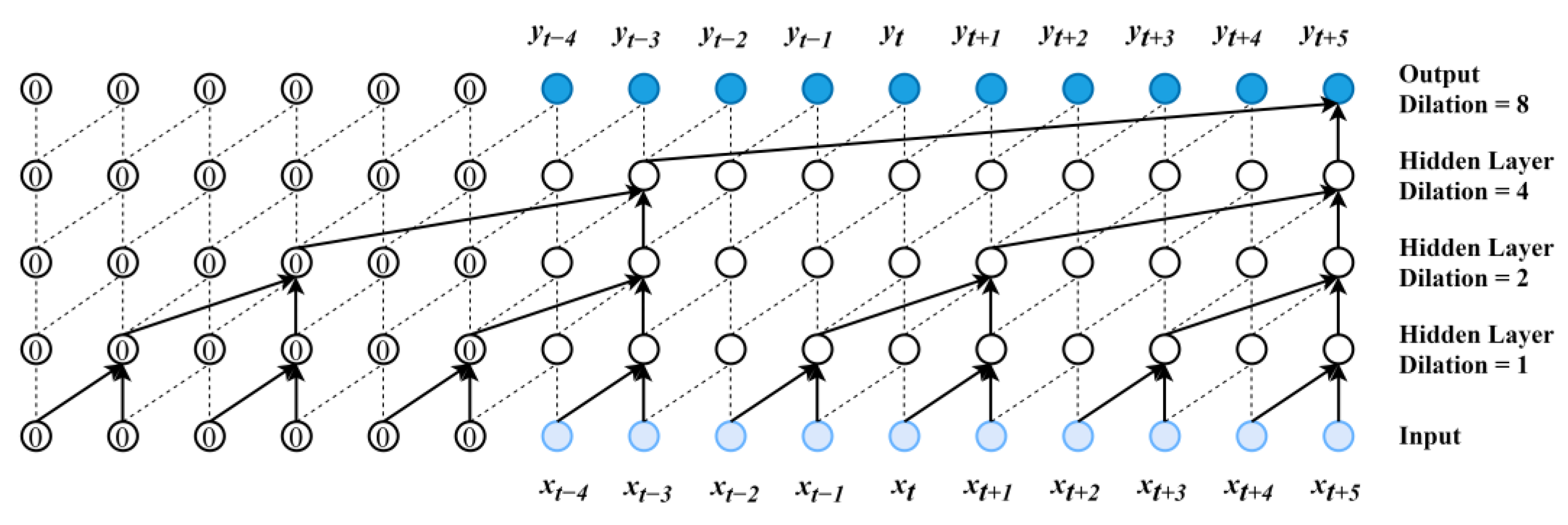
Figure 1 shows a causal convolution structure in which the output at time t + 5 is related only to $x_{\mathrm{t}-4}, \dots ,x_{\mathrm{t}}, x_{t+5}$. In addition, to allow the TCN to have a wider receptive field, a dilation convolution structure was applied to the TCN model. Figure 2 shows the dilated causal convolution structure with expansion numbers of 1, 2, 4, and 8, which has a receptive field of 10 time steps using four convolution operations. Additionally, to maintain the same spatial dimension of the input and output, 0 was added before the beginning of the time series.

2.2.2. Multi-Nuclide Source Term Inversion Model Based on TCN

The inversion model of multi-nuclide source terms for nuclear accidents constructed based on TCN units is shown in Figure 3.

(a) 

First, the gamma dose rate data from the two monitoring points are pre-processed by converting the gamma dose rate for 10 h into a 10 × 10 matrix, i.e., the first row is the gamma dose rate at time step 1, the tenth row is the gamma dose rate at time steps 1 to 10, and all missing data are filled with the default value “0”.

(b) 

To avoid the distortion effects of using default values, a masking unit [30] was used to mask the fixed values in the input sequence signal, locating the time steps to be skipped. If the input data are equal to the given value, the time step is omitted in all the subsequent layers of the model. As shown in Figure 3c, only one valid data point remains in the first row after processing through the mask unit.

(c) 

The gamma dose rate at the tenth time step was used as an example. Sequence information of the gamma dose rate was extracted using the TCN. Feature extraction of gamma dose rate data from two monitoring points was done using n convolution kernels. The nonlinear activation function of the data features was computed by the ReLU activation function, which introduced nonlinear elements to the neurons and allowed the neural network to approximate any other nonlinear function. The deep network was dispersed to avoid overfitting by the weight regularization layer [31] and the dropout layer [32].

(d) 

Gamma dose rate data, release height, atmospheric stability, wind speed, mixed layer height, and precipitation type were combined as input data.

(e) 

Input data were fed to the full connection layer, and the release rates of the seven nuclides were output.

2.3. Inversion Model Based on 2D-CNN

The extraction of one-dimensional time series features can be directly analyzed using recurrent neural networks and time series CNNs. Recent studies have shown that a one-dimensional time series signal can be transformed into two-dimensional image data via polar coordinate conversion. Feature extraction was then performed using a 2D-CNN. There was a significant improvement in prediction accuracy for several experiments [26].

2.3.1. Gramian Angular Field

The Gramian angular field [26] is used to encode the time series into images. The one-dimensional time series was converted from Cartesian to polar coordinates. It was then converted into a two-dimensional image by the operation of the Gramian matrix. In addition, it could also be converted to the original time series by an inverse operation with good interpretability. The Gramian angular field was processed as follows:

(1)

First, the one-dimensional time series was normalized, and the normalized time series was denoted by $X$.

(2)

The timestamp of $X$ was then used as the radius. The value corresponding to the time stamp was used as the cosine angle. The $X$ was re-projected to polar coordinates based on the radius and cosine angle.

(3)

Finally, $X$ was converted into a Gramian angular summation field (GASF) in image format based on the sum of the trigonometric functions between each point. The $X$ was converted into a Gramian angular difference field (GADF) based on the difference in trigonometric functions. GASF and GADF are defined in Equations (2) and (3).

$$GASF=\left[\cos \left({\varphi }_i+{\varphi }_j\right)\right]=X_i\cdot X_j-\sqrt{I-X_i{}^2\cdot }\sqrt{I-X_j{}^2}$$

(2)

$$GADF=\left[\sin \left({\varphi }_i+{\varphi }_j\right)\right]=X_i·\sqrt{I-X_j{}^2}-\sqrt{I-X_i{}^2}·X_j$$

(3)

where $I$ represents the unit vector in polar coordinates and $\varphi$ is the angle between the two time vectors.

2.3.2. 2D-CNN Algorithm

A CNN is a deep feedforward network that has been successfully used in image fields, such as image classification and retrieval, and target detection and segmentation [33]. A 2D-CNN generally consists of three structures: a convolutional layer, a pooling layer, and a fully connected layer.

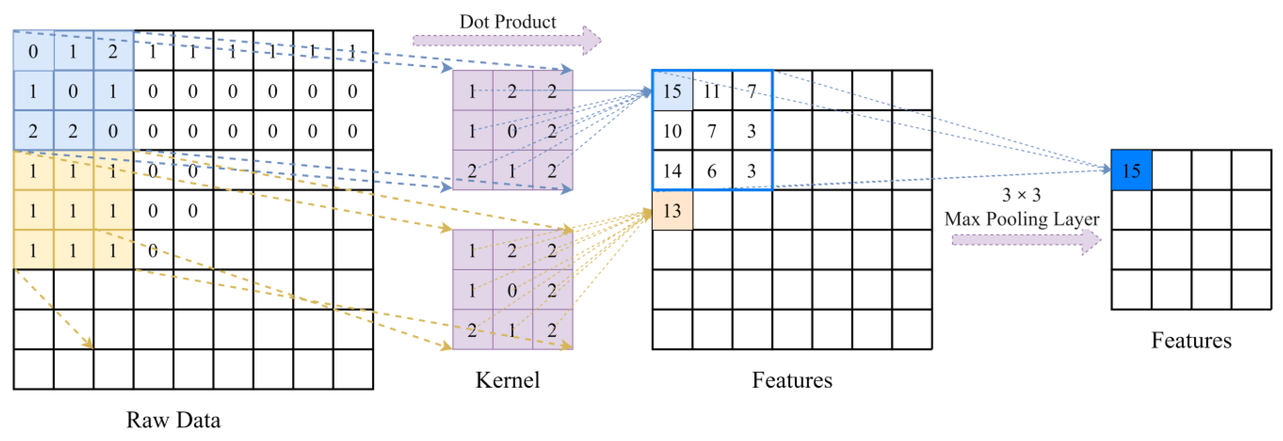
The convolutional layer, as the core of the CNN, consists of several feature planes that extract different features from the input through convolutional operations. The first convolutional layer extracts low-level features, such as edges, lines, and corners. Higher-level convolutional layers extract higher-level features [34]. As shown in Figure 4, the convolutional kernel slides on the input image sequentially, and the sliding direction is from left to right and from top to bottom. For each slide, convolution performs a dot product calculation with the input image corresponding to its sliding window position, which preserves the spatial features of the input image. The max pooling layer compresses images, mainly to speed up the convergence process of neural networks and improve the stability of the training process [35]. In the CNN structure, after multiple convolutional and sampling layers, one or more fully connected layers are connected, and each neuron in the fully connected layer is fully connected to all the neurons in the layer before it. Fully connected layers can integrate local information with category differentiation in the convolutional or sampling layers.

2.3.3. Multi-Nuclide Source Term Inversion Model Based on 2D-CNN

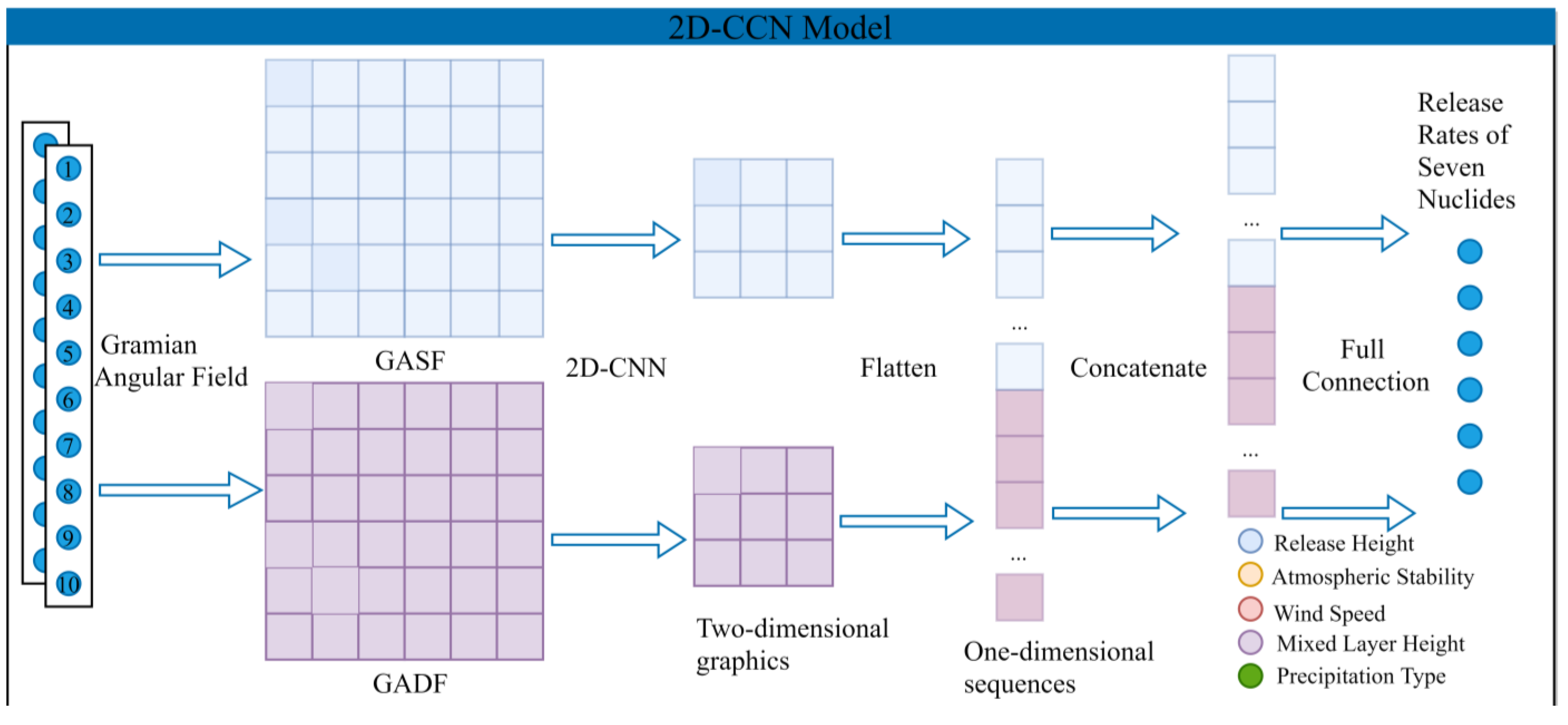
The inversion model of the multi-nuclide source term for nuclear accidents, constructed based on 2D-CNN units, is shown in Figure 5. First, the gamma dose rates of the two monitoring points were input and transformed by the Gramian angular field to form two two-dimensional images. Then, 2D-CNN layers were used for feature extraction, while weight regularization, pooling, and dropout were used to disperse the deep network to avoid overfitting. Next, after flattening the multi-dimensional data into one-dimensional data, they were connected to five auxiliary data points. Finally, the data were fed into the fully connected layer, and the release rates of the seven nuclides were output.

2.4. Model Fusion Method Based on Improved Bagging Method

Model fusion, also known as ensemble learning [36], is used to accomplish learning tasks by constructing and combining multiple base learners. The main premise is that by combining multiple models, the deviation of a single base learner may be compensated for by other base learners. As a result, the overall prediction performance of the ensemble learner will outperform that of the single base learner, allowing the model to have better generalization capabilities.

2.4.1. Bagging

The main idea of bagging, also known as bootstrap aggregation, is to generate a series of independent observed data of the same size and distribution as the original data. Subsequently, multiple base learners are constructed based on the observed data, and the output of the base learners is used as the input of the meta learner. The process of constructing a fusion model using the bagging method is as follows:

(1)

First, $n$ times with put-back sampling is performed from the training dataset $M$ of size $n$ to obtain dataset $M_1$, which is repeated $N$ times to obtain $N$ datasets $M_1,\dots ,M_N$ of size $n$.

(2)

Then, $N$ base algorithm models are selected, and $N$ base learners are constructed with the input data set $M_1,\dots ,M_N$.

(3)

Finally, the output of the fusion model is obtained by linearly averaging the output of each base learner.

2.4.2. Multi-Nuclide Source Term Inversion Model Based on Fusion Model

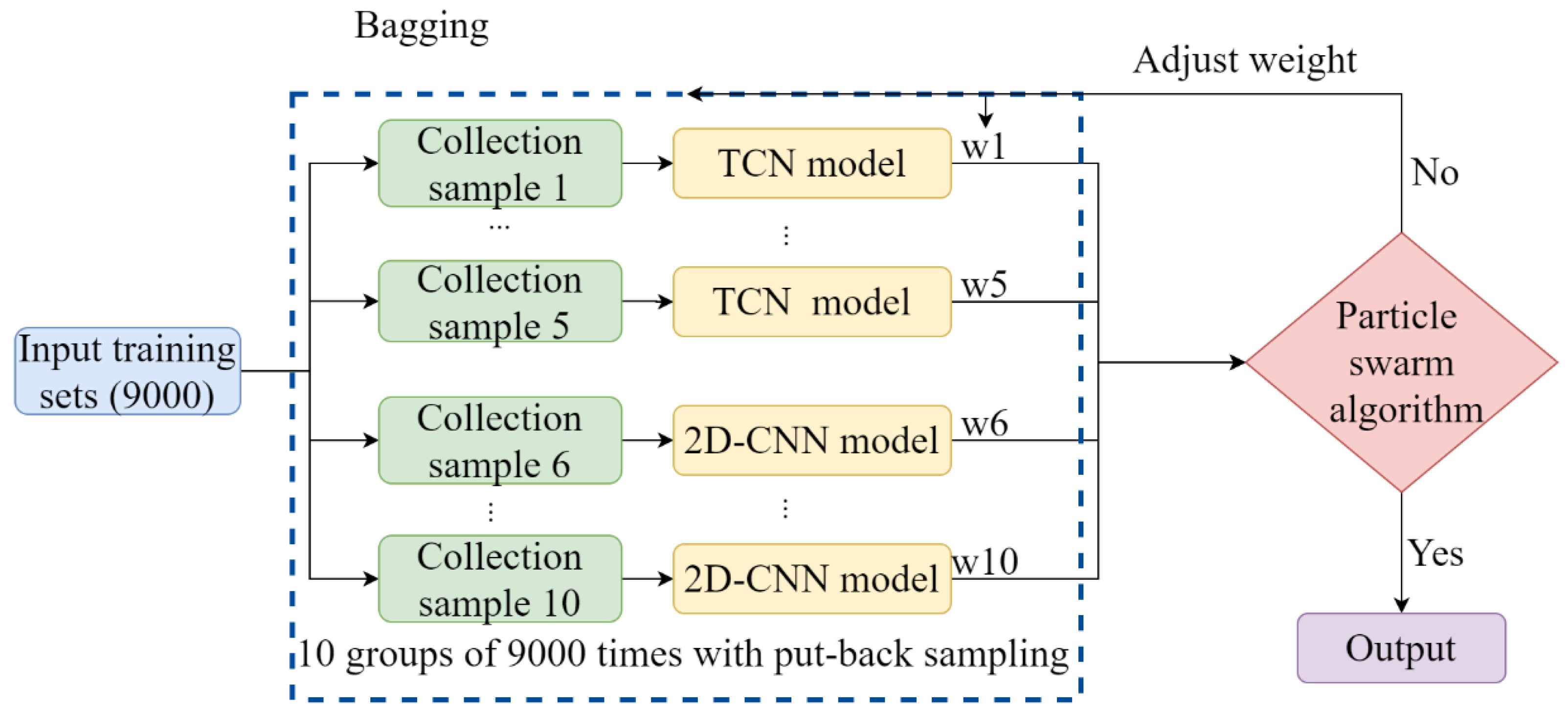
As shown in Figure 6, the original 9000 sets of training datasets were randomly drawn 9000 times in a putback form, meaning that a set of training datasets can be drawn repeatedly, which will form a new collection with 9000 training datasets. The above process was repeated 10 times to form 10 new collections. Five used the TCN model as the base learner, and the other five used the 2D-CNN model. The weights of the base learners in the model were adjusted using a particle swarm optimization (PSO) algorithm, and the output of each base learner was multiplied by its weight separately as the output of the fusion model to obtain the final prediction results.

2.5. BOHB Algorithm

The hyperparameters of deep learning typically interact with each other, and it is often difficult to obtain optimal results using the single-variable method. Black-box optimization models based on Bayesian optimization have excellent performance in several deep learning tuning tasks [37], and Bayesian optimization can theoretically approximate optimal results [38]; however, exponential explosions often occur when applied to high-latitude computations. The BOHB algorithm [39], combined with the probabilistic sampling of Bayesian optimization and the step-by-step halving process of hyperband optimization, plays an important role in determining the number of groups of hyperparameters to run and the budget allocated to each group. To avoid the effects caused by random parameter selection, the Bayesian optimization model helps the hyperband optimization algorithm to select parameters at the beginning of each cycle using previously available data. Once the hyperparameters generated by the Bayesian optimization reach the required number of configurations for the iteration, these configurations are used to start the successive halving operation. Successive halving operations can effectively reduce search time and cover a wider search space in less time.

In this study, BOHB was used to optimize the number of convolutional kernels, convolutional kernel width, number of fully connected layer neurons, and batch size for the TCN and 2D-CNN models.

2.6. PSO Algorithm

The PSO [40] is an optimization algorithm based on an iterative model that was initially used for optimization in continuous spaces. In the continuous space coordinate system, the mathematical description of the particle swarm algorithm is as follows: A population of m particles travels at a certain speed in a D-dimensional search space, and each particle varies its position based on its own search for the historical best point and the historical best points of other particles in the population when searching. The $i$th particle of the particle swarm is composed of three D-dimensional vectors: current position ($x_i=\left(x_{i1}, x_{i2}, \dots , x_{iD}\right)$), historical optimal position ($x_i=\left(x_{i1}, x_{i2}, \dots , x_{iD}\right)$), and speed ($v_i=\left(v_{i1}, v_{i2}, \dots , v_{iD}\right)$), where $i=1, 2,\dots , n$. The current position is considered a set of coordinates describing a spatial point, and at each iteration of the algorithm, the current position $x_i$ is evaluated as the problem solution. If the current position is better than the historical optimal position $p_i$, a second vector $p_i$ exists for the coordinates of the target position. In addition, the best position searched thus far in the whole particle swarm is denoted as $p_g=\left(p_{g1}, p_{g2}, \dots , p_{gD}\right)$.

In this study, the PSO algorithm was used to optimize the weights of the fusion model. The PSO was built using Sko [41], an advanced wrapper package in Python 3.7.

2.7. Estimation Metrics

To assess the overall performance of the model, estimation metrics are required to verify the effectiveness of the model; therefore, the following four evaluation metrics were selected in this study. (1) The loss values were set to the mean squared error (MSE). (2) The mean absolute error (MAE) was used to assess the overall performance of the model. (3) Two metrics, namely, absolute percentage error (APE). (4) Mean absolute percentage error (MAPE), were used to reflect the estimation performance more intuitively. These metrics are calculated as follows:

$$Loss=MSE=\frac{1}{m}{{\displaystyle \sum }}_{i=1}^m{\left(f_i-y_i\right)}^2$$

(4)

$$MAE=\frac{1}{m}{{\displaystyle \sum }}_{i=1}^m\left|f_i-y_i\right|$$

(5)

$$APE=\frac{\left|f_i-y_i\right|}{y_i}$$

(6)

$$MAPE=\frac{1}{m}{{\displaystyle \sum }}_{i=1}^m\frac{\left|f_i-y_i\right|}{y_i}$$

(7)

where $y_i$ is the true value, $f_i$ the predicted value of the model, and $m$ the number of samples in the dataset.

3. Results

3.1. Hyperparameter Optimization of TCN and 2D-CNN Models

Hyperparameters set for the models before starting the learning process play a significant role in improving the performance and effectiveness of neural network learning. Therefore, it is necessary to optimize these parameters to obtain a preferable set of hyperparameters.

3.1.1. Learning Rate

The learning rate is a hyperparameter that updates the weights during gradient descent; that is $\eta$ of the following equation:

$${\omega }^{n+1}={\omega }^n-\eta \times \frac{\partial L\left({\omega }^n\right)}{\partial {\omega }^n}$$

(8)

where ${\omega }^n$ is the neural network weight at moment $n$, ${\omega }^{n+1}$ is the weight at moment $n+1$, and L is the loss function (MSE). Thus, the learning rate $\eta$ directly determines the update rate of the neural network weights. At a low learning rate, the update rate of the loss function is slow, which easily leads to overfitting of the model. At a high learning rate, the loss function will vibrate substantially, and the model is prone to gradient explosion, leading to difficulty in convergence of the model. Therefore, it is important to select a suitable learning rate.

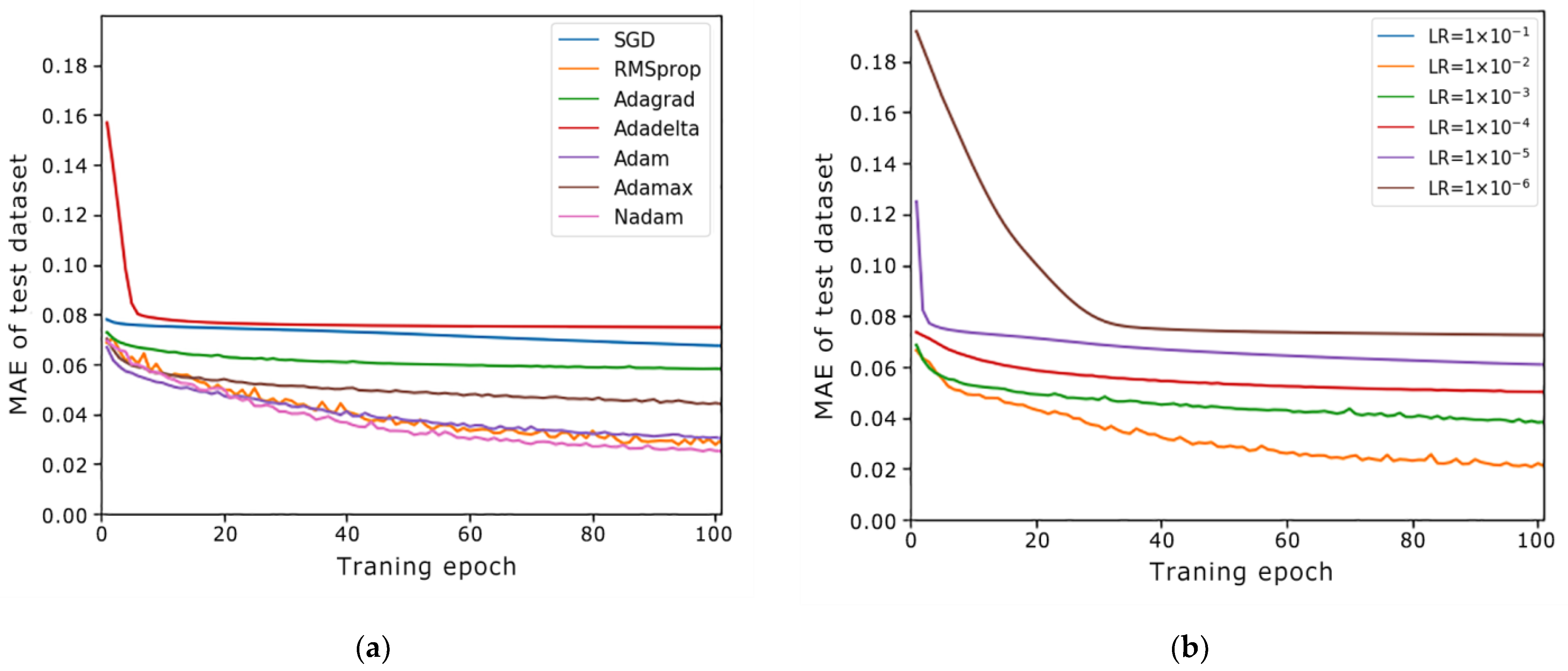
In Keras, which is a neural network kit [42], the learning rate is set within the optimizer; therefore, it is necessary to first select an optimal optimizer from among the seven optimizers (as shown in Figure 7a) and subsequently choose the best learning rate based on the best optimizer. When selecting the best optimizer, other hyperparameters were set to the default values of Keras.

From Figure 7a, the lowest MAE was obtained with the optimizer of Nadam for the 2D-CNN model when the number of training epochs reached 100. Therefore, the preferable learning rate of 10⁻² from the optimizer of Nadam can be determined from Figure 7b. Similarly, the best optimizer for the TCN model was Nadam and the best learning rate was 10⁻².

3.1.2. Other Hyperparameters

In addition to the learning rate, there are four important parameters that have a significant impact on the prediction accuracy of the models: number of convolutional kernels, width of convolutional kernels, number of fully connected layer neurons, and batch size. These were adjusted using the BOHB algorithm in the ranges listed in

Table 4. Parameter search range based on 2D-CNN and TCN models.

Parameter	Value Range
Number of convolutional kernels	0–64
Width of convolutional kernels	2, 4, 8
Number of fully connected layer neurons	8–256

.

From Figure 8, a parallel coordinate plot of the combinations of the four parameters and their corresponding MAE shows that the lowest MSE of the 2D-CNN model corresponding to these parameters can be below 0.02, which indicates that the BOHB algorithm can reduce the prediction deviation of the model compared to the model without tuning the parameters. The best configurations for the 2D-CNN model searched by BOHB are listed in

Table 5. Optimal parameter values of multi-nuclide source term inversion model based on 2D-CNN and TCN.

Model	Optimizer	Learning Rate	Number of Convolution Kernels	Convolution Kernel Width	Fully Connected Layers Number of Neurons	Batch Size	Loss
2D-CNN	Nadam	10−2	48	2	96	128	0.0138
TCN	Nadam	10−2	40	8	48	2048	0.0196

. Similarly, the best configurations for the TCN model were obtained, as listed in Table 5.

3.1.3. Multi-Nuclide Emission Rate Estimation Performance of TCN and 2D-CNN Models

As shown in Figure 9, the MAPE of the release rate from both the TCN and 2D-CNN models decreased rapidly in the first few steps. For the TCN model, the MAPEs for all nuclides falls below 30% when the time step reaches the fourth hour. Among them, the MAPEs for Kr-88 and Te-132 reached approximately 10%. For the 2D-CNN model, when the time step reached the sixth hour, the MAPEs for all nuclides fall below 30%, and only the MAPE for Kr-88 can reach below 10%; however, for the other nuclides, the MAPEs can reach below 20% in the final time step. In the initial period, the results from the TCN model were superior to those from the 2D-CNN model. This is because when the length of the sequence is short, the Gramian angular field expanding the one-dimensional sequence into two dimensions leads to distortion of the original information. This indicates that the TCN model has a strong prediction ability using less gamma dose rate data because of its strong feature extraction ability of convolutional operation, which is important for rapid estimation of the source term after a nuclear accident. In addition, the 2D-CNN model has a lower prediction deviation at the final time step because the feature extraction ability of two-dimensional convolution is stronger than that of one-dimensional convolution, which can provide more reliable prediction results.

Thus, it can be helpful to improve the prediction accuracy if the two models can be effectively fused.

3.2. Fusion of TCN and 2D-CNN Models Based on Bagging Method

3.2.1. Weight Optimization through PSO Algorithm

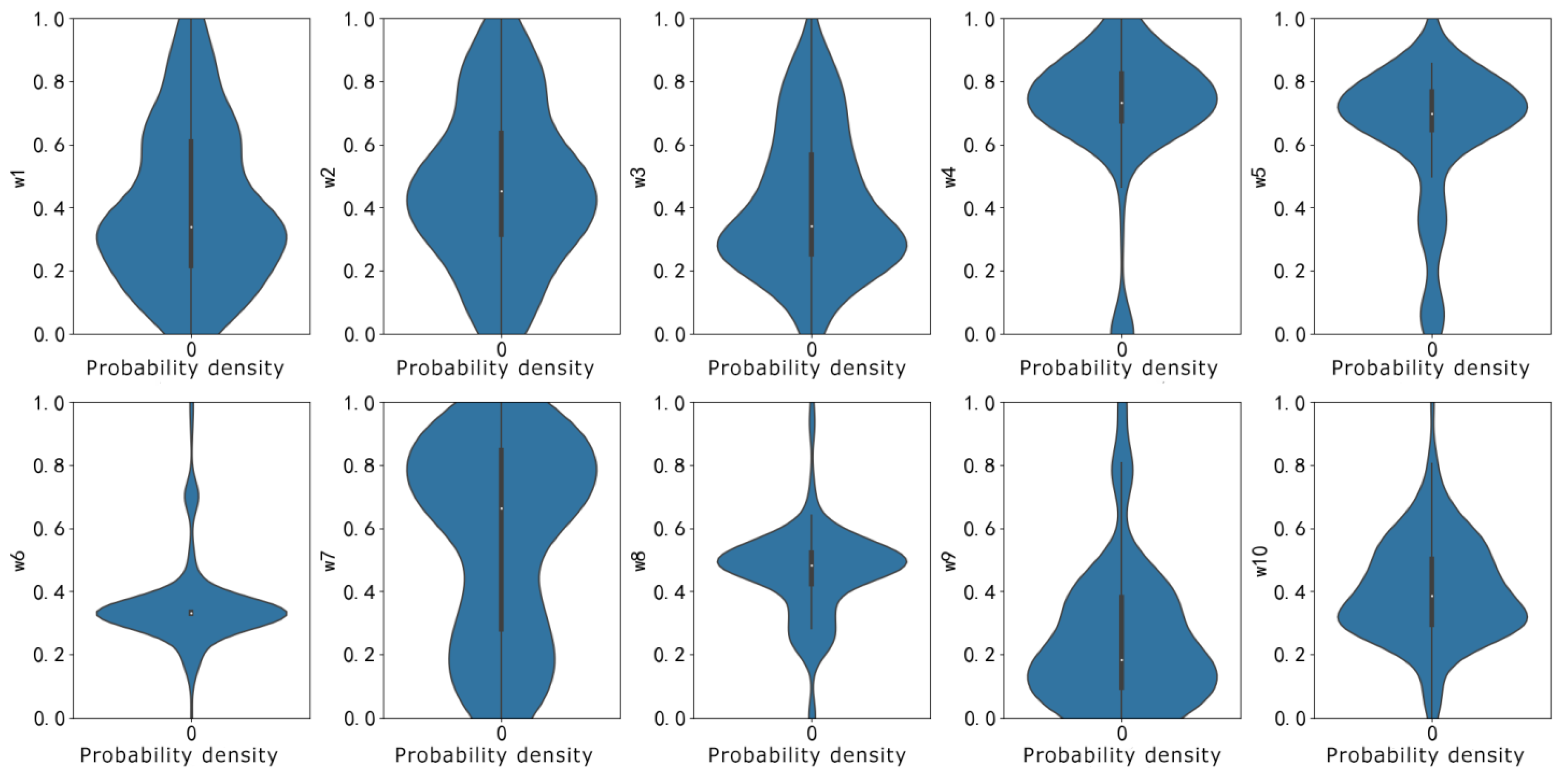
As shown in Figure 6, before 10 re-sampled datasets are fed into the fusion model, their respective weights should be determined because different combinations of the 10 weights will affect the fusion result. The determination process is performed using the PSO algorithm, which searches for weights between 0 and 1.

Figure 10 shows the probability distribution of each weight in the PSO search process, in which the ordinate values at the widest positions in the shapes are the best weights because when the weights take these values, the probability of obtaining a low prediction deviation is the highest. Thus, the optimal weights searched by the PSO algorithm and the corresponding loss values were determined, as listed in

Table 6. Optimal weighting values searched by particle swarm search algorithm.

Base Learner	Weight	Value	Base Learner	Weight	Value
TCN	w1	0.39	2D-CNN	w6	0.37
TCN	w2	0.48	2D-CNN	w7	0.21
TCN	w3	0.32	2D-CNN	w8	0.52
TCN	w4	0.76	2D-CNN	w9	0.14
TCN	w5	0.71	2D-CNN	w10	0.42
Fusion Model	Loss: 0.0082

.

3.2.2. Multi-Nuclide Emission Rate Estimation Performance

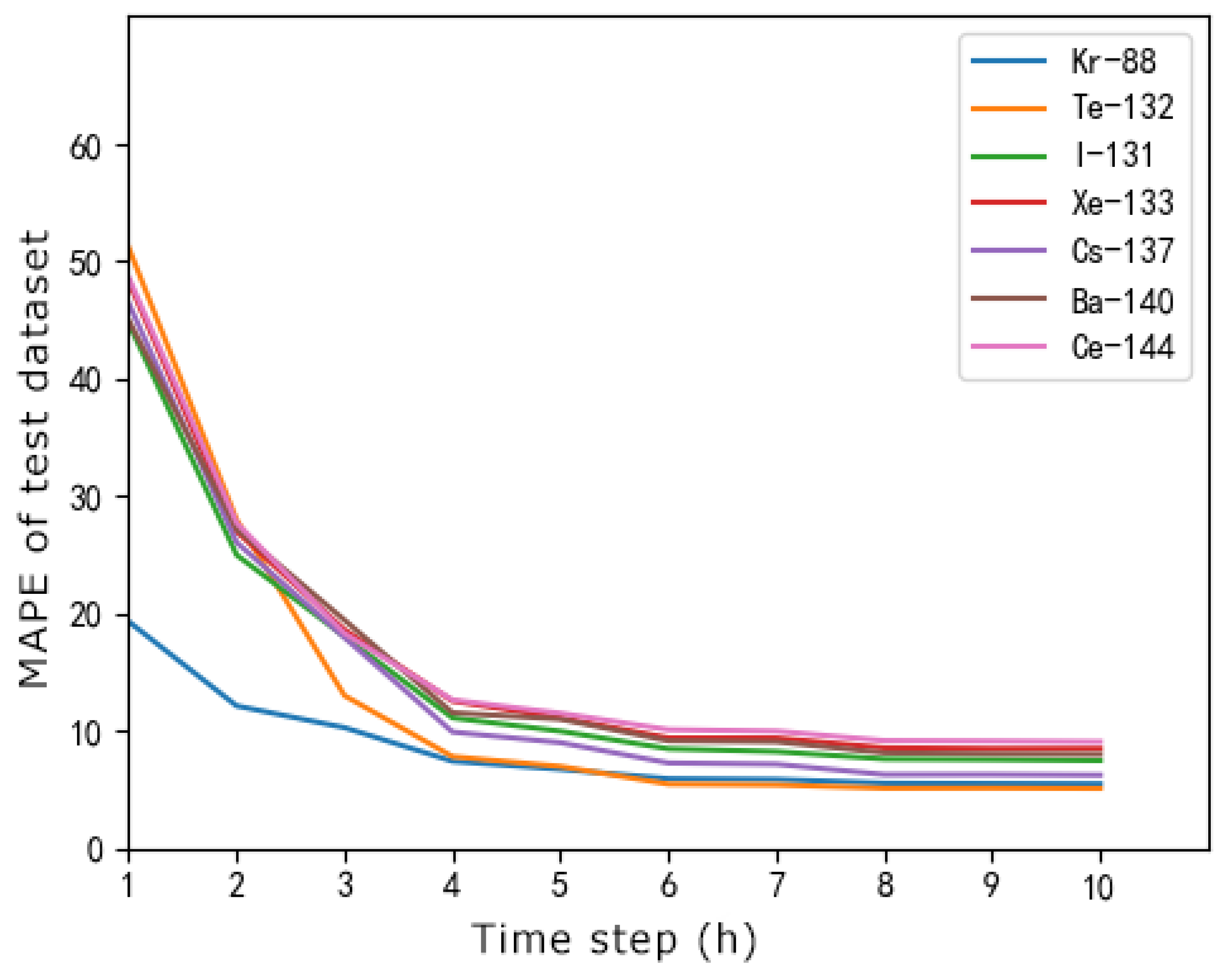
The MAPEs with time steps for the seven nuclides obtained by the fusion model in the test dataset are shown in Figure 11. It was observed that the MAPEs at the fourth hour all decreased below 20%, and all of them reached below 10% at the final time step. The MAPEs of the predicted values of Kr-188 and Te-132 were 7.1% and 5.2%, respectively.

Compared with the results of the TCN or 2D-CNN models, the MAPEs obtained with the fusion model showed a significant decrease in both the fifth and final time steps. This suggests that the fusion model, which inherits the advantages of the TCN and 2D-CNN models, effectively improves the prediction ability. The MAPE values of the seven nuclides at the final time step are listed in

Table 7. The MAPE of seven nuclides predicted by each model at the final time step.

Model	MAPE (%)
TCN	17.31
2D-CNN	14.53
Fusion Model	8.64

.

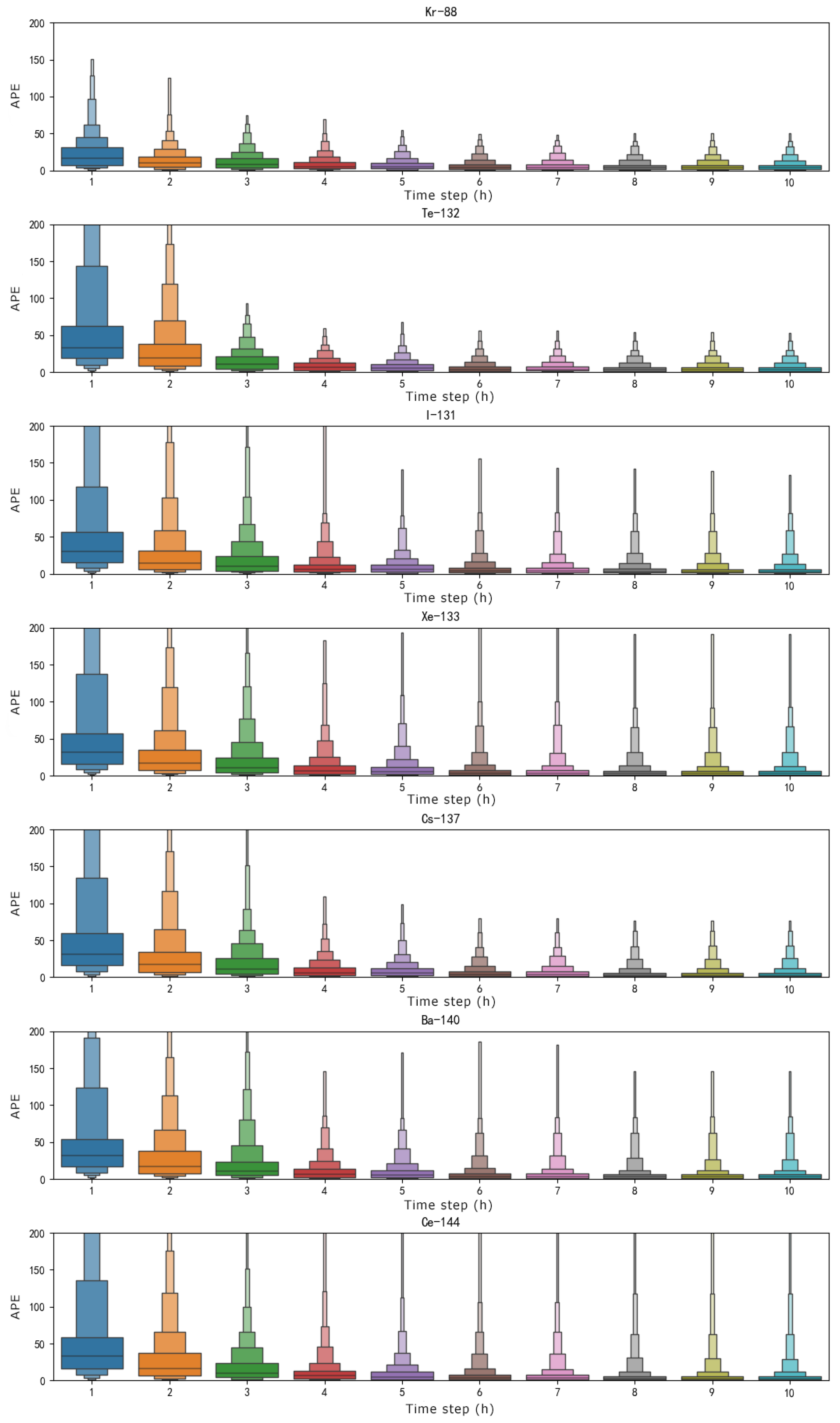
In Figure 12, an enhanced box plot, shows a detailed APE distribution over time for all data samples in the test dataset. There are several black horizontal lines, called quantiles, in each shape, which represent the quantiles of 1/2, 1/4, 1/8, 1/16, 1/32, 1/64, and 1/128. As shown in Figure 12, at the first time step, when inputting only one hour of gamma dose rate data, more than 1/8 of the samples for all nuclides (except Kr-88) have an APE over 100%. At the third time step, most samples of Kr-88 and Te-132 have an APE below 50%. At the final time step, although a small percentage of samples have high APEs, all medians are located at a very low level. Additionally, in the last three time steps, the shapes barely change, which suggests that 10 h of gamma dose rate data are sufficient for the source term inversion model.

3.3. Noise Analysis

In practical situations, all measurement data are inevitably biased, and the robustness of the model can be verified by adding noise to the input data. As shown in Figure 13, the performance of the fusion model in estimating the multi-nuclide release rate was examined by adding 1–50% noise to the input data for the final time step. Noise analysis was performed for the input parameters of gamma dose rate, wind speed, release height, and mixed layer height.

As shown in Figure 13, the MAPE increases significantly with an increase in the gamma dose rate, which indicates that the noise of the gamma dose rate significantly affects the estimation of multi-nuclide release rates. Among the four input parameters, the gamma dose rate is the most important input for estimating multi-nuclide release rates. The MAPE of most nuclides from the noise of the gamma dose rate can be maintained at approximately 30%, with good robustness of the fusion model at a relative noise level of 10%.

As shown in Figure 13b,c, the noise at release and mixed layer heights had little effect on the estimation of the multi-nuclide release rate, and the MAPE of most radionuclides increased slowly with noise, remaining below 15%, even at a 50% noise level.

Wind speed is a key parameter in the diffusion of all nuclides. As shown in Figure 13d, for all nuclides (except Kr-88), the MAPEs remained below 20%, even at a 50% noise level. The estimation of Kr-88 is more sensitive to the noise of wind speed than to that of the gamma dose rate because it is a radioactive gas and has a short half-life (2.84 h).

4. Conclusions

In this study, an inversion method is proposed for multiple nuclide source terms in nuclear accidents based on a deep learning fusion model. It can further improve prediction accuracy compared with TCN and 2D-CNN models when performing the inversion under an assumed situation with a homogeneous release of seven nuclides and constant meteorological conditions. The MAPE of the fusion model at the final time step using the weights optimized by the PSO algorithm can reach below 10%.

Additionally, the prediction performance of the fusion model was tested by adding noise to the input data. The results show that the fusion model is not sensitive to the noise of meteorological conditions; however, the noise of the gamma dose rate has a significant impact on the prediction of the fusion model. When there is 20% noise in the gamma dose rate, the prediction deviation of the fusion model for the nuclide release rate is approximately 30%; therefore, it suggests that it is important to obtain gamma dose rate data as accurately as possible to improve the estimation performance of the fusion model.

References

1. Chen, D. Nuclear energy and nuclear safety: Analysis and reflection on the Fukushima nuclear accident in Japan. J. Nanjing Univ. Aeronaut. Astronaut. 2012, 44, 597–602. [Google Scholar]
2. Kathirgamanathan, P.; McKibbin, R.; McLachlan, R.I. Source Release-Rate Estimation of Atmospheric Pollution from a NonSteady Point Source at a Known Location. Environ. Model. Assess. 2004, 9, 33–42. [Google Scholar] [CrossRef]
3. Liu, Y. Research on Inversion Model of Nuclear Accident Source Terms Based on Variational Data Assimilation. Ph.D. Thesis, Tsinghua University, Beijing, China, 2017. [Google Scholar]
4. Katata, G.; Ota, M.; Terada, H.; Chino, M.; Nagai, H. Atmospheric discharge and dispersion of radionuclides during the Fukushima Dai-ichi Nuclear Power Plant accident. Part I: Source term estimation and local-scale atmospheric dispersion in early phase of the accident. J. Environ. Radioact. 2012, 109, 103–113. [Google Scholar] [CrossRef] [PubMed] [Green Version]
5. Du Bois, P.B.; Laguionie, P.; Boust, D.; Korsakissok, I.; Didier, D.; Fiévet, B. Estimation of marine source-term following Fukushima Daiichi accident. J. Environ. Radioact. 2021, 114, 2–9. [Google Scholar] [CrossRef]
6. Liu, Y.; Liu, X.; Li, H.; Fang, S.; Mao, Y.; Qu, J. Research on Source Inversion for Nuclear Accidents Based on Variational Data Assimilation with the Dispersion Model Error. In Proceedings of the 2018 26th International Conference on Nuclear Engineering, London, UK, 22–26 July 2018. [Google Scholar] [CrossRef]
7. Tsiouri, V.; Andronopoulos, S.; Kovalets, I.; Dyer, L.L.; Bartzis, J.G. Radiation source rate estimation through data assimilation of gamma dose rate measurements for operational nuclear emergency response systems. Int. J. Environ. Pollut. 2012, 50, 386–395. [Google Scholar] [CrossRef]
8. Tsiouri, V.; Kovalets, I.; Andronopoulos, S.; Bartzis, J. Emission rate estimation through data assimilation of gamma dose measurements in a Lagrangian atmospheric dispersion model. Radiat. Prot. Dosim. 2011, 148, 34–44. [Google Scholar] [CrossRef]
9. Drews, M.; Lauritzen, B.; Madsen, H.; Smith, J.Q. Kalman filtration of radiation monitoring data from atmospheric dispersion of radioactive materials. Radiat. Prot. Dosim. 2004, 111, 257–269. [Google Scholar] [CrossRef]
10. Zhang, X.; Su, G.; Yuan, H.; Chen, J.; Huang, Q. Modified ensemble Kalman filter for nuclear accident atmospheric dispersion: Prediction improved and source estimated. J. Hazard. Mater. 2014, 280, 143–155. [Google Scholar] [CrossRef]
11. Zavisca, M.; Kahlert, H.; Khatib-Rahbar, M.; Grindon, E.; Ang, M. A Bayesian Network Approach to Accident Management and Estimation of Source Terms for Emergency Planning. In Probabilistic Safety Assessment and Management; Springer: London, UK, 2004. [Google Scholar] [CrossRef]
12. Zheng, X.; Itoh, H.; Kawaguchi, K.; Tamaki, H.; Maruyama, Y. Application of Bayesian nonparametric models to the uncertainty and sensitivity analysis of source term in a BWR severe accident. Reliab. Eng. Syst. Saf. 2015, 138, 253–262. [Google Scholar] [CrossRef]
13. Davoine, X.; Bocquet, M. Inverse modelling-based reconstruction of the Chernobyl source term available for long-range transport. Atmos. Chem. Phys. 2007, 7, 1549–1564. [Google Scholar] [CrossRef] [Green Version]
14. Jeong, H.-J.; Kim, E.-H.; Suh, K.-S.; Hwang, W.-T.; Han, M.-H.; Lee, H.-K. Determination of the source rate released into the environment from a nuclear power plant. Radiat. Prot. Dosim. 2005, 113, 308–313. [Google Scholar] [CrossRef] [PubMed]
15. Ruan, Z.; Zhang, S. Simultaneous inversion of time-dependent source term and fractional order for a time-fractional diffusion equation. J. Comput. Appl. Math. 2020, 368, 112566. [Google Scholar] [CrossRef]
16. Tichý, O.; Šmídl, V.; Hofman, R.; Evangeliou, N. Source term estimation of multi-specie atmospheric release of radiation from gamma dose rates. Q. J. R. Meteorol. Soc. 2018, 144, 2781–2797. [Google Scholar] [CrossRef]
17. Zhang, X.; Raskob, W.; Landman, C.; Trybushnyi, D.; Li, Y. Sequential multi-nuclide emission rate estimation method based on gamma dose rate measurement for nuclear emergency management. J. Hazard. Mater. 2017, 325, 288–300. [Google Scholar] [CrossRef] [PubMed]
18. Zhang, X.; Raskob, W.; Landman, C.; Trybushnyi, D.; Haller, C.; Yuan, H. Automatic plume episode identification and cloud shine reconstruction method for ambient gamma dose rates during nuclear accidents. J. Environ. Radioact. 2017, 178, 36–47. [Google Scholar] [CrossRef]
19. Fang, S.; Dong, X.; Zhuang, S.; Tian, Z.; Chai, T.; Xu, Y.; Zhao, Y.; Sheng, L.; Ye, X.; Xiong, W. Oscillation-free source term inversion of atmospheric radionuclide releases with joint model bias corrections and non-smooth competing priors. J. Hazard. Mater. 2022, 440, 129806. [Google Scholar] [CrossRef]
20. Li, X.; Sun, S.; Hu, X.; Huang, H.; Li, H.; Morino, Y.; Wang, S.; Yang, X.; Shi, J.; Fang, S. Source inversion of both long- and short-lived radionuclide releases from the Fukushima Daiichi nuclear accident using on-site gamma dose rates. J. Hazard. Mater. 2019, 379, 120770. [Google Scholar] [CrossRef]
21. Sun, S.; Li, X.; Li, H.; Shi, J.; Fang, S. Site-specific (Multi-scenario) validation of ensemble Kalman filter-based source inversion through multi-direction wind tunnel experiments. J. Environ. Radioact. 2019, 197, 90–100. [Google Scholar] [CrossRef] [PubMed]
22. Ling, Y.; Yue, Q.; Chai, C.; Shan, Q.; Hei, D.; Jia, W. Nuclear accident source term estimation using Kernel Principal Component Analysis, Particle Swarm Optimization, and Backpropagation Neural Networks. Ann. Nucl. Energy 2020, 136, 107031. [Google Scholar] [CrossRef]
23. Yue, Q.; Jia, W.; Huang, T.; Shan, Q.; Hei, D.; Zhang, X.; Ling, Y. Method to determine nuclear accident release category via environmental monitoring data based on a neural network. Nucl. Eng. Des. 2020, 367, 110789. [Google Scholar] [CrossRef]
24. Ling, Y.; Yue, Q.; Huang, T.; Shan, Q.; Hei, D.; Zhang, X.; Jia, W. Multi-nuclide source term estimation method for severe nuclear accidents optimized by Bayesian optimization and hyperband. J. Hazard. Mater. 2021, 414, 125546. [Google Scholar] [CrossRef] [PubMed]
25. Ling, Y.; Huang, T.; Yue, Q.; Shan, Q.; Hei, D.; Zhang, X.; Shi, C.; Jia, W. Improving the estimation accuracy of multi-nuclide source term estimation method for severe nuclear accidents using temporal convolutional network optimized by Bayesian optimization and hyperband. J. Environ. Radioact. 2022, 242, 106787. [Google Scholar] [CrossRef] [PubMed]
26. Hong, Y.Y.; Martinez, J.J.F.; Fajardo, A.C. Day-ahead solar irradiation forecasting utilizing gramian angular field and convolutional long short-term memory. IEEE Access 2020, 8, 18741–18753. [Google Scholar] [CrossRef]
27. Till, J.E.; Meyer, H.R. Radiological Assessment. A Textbook on Environmental Dose Analysis; Oak Ridge National Lab.: Oak Ridge, TN, USA, 1983. [Google Scholar] [CrossRef] [Green Version]
28. Malamud, H. Reactor Safety Study—An Assessment of Accident Risks. U.S.; Nuclear Regulatory Commission: Rockville, MD, USA, 1975. [Google Scholar] [CrossRef] [Green Version]
29. Bai, S.; Kolter, J.Z.; Koltun, V. An Empirical Evaluation of Generic Convolutional and Recurrent Networks for Sequence Modeling. arXiv 2018. [Google Scholar] [CrossRef]
30. Yang, H.; Yin, L. CNN based 3D facial expression recognition using masking and landmark features. In Proceedings of the 2017 Seventh International Conference on Affective Computing and Intelligent Interaction (ACII), San Antonio, TX, USA, 23–26 October 2017. [Google Scholar]
31. Yin, R.; Shu, S.; Li, S. An image moment regularization strategy for convolutional neural networks. CAAI Trans. Intell. Syst. 2016, 11, 43–48. [Google Scholar]
32. Baldi, P.; Sadowski, P.J. Understanding dropout. Adv. Neural Inf. Proc. Syst. 2013, 26, 2814–2822. [Google Scholar]
33. Chao, L.; Chen, W.; Yu, L.; Changfeng, X.; Xiufeng, Z. A review of structural optimization of convolutional neural networks. Acta Autom. Sin. 2020, 46, 24–37. [Google Scholar]
34. Peng, X.; Zhang, B.; Gao, D. Research on fault diagnosis method of rolling bearing based on 2DCNN. In Proceedings of the 2020 Chinese Control and Decision Conference (CCDC), Hefei, China, 22–24 August 2020; Volume 8, pp. 2–24. [Google Scholar] [CrossRef]
35. Jie, H.J.; Wanda, P. RunPool: A dynamic pooling layer for convolution neural network. Int. J. Comput. Intell. Syst. 2020, 13, 66–76. [Google Scholar] [CrossRef] [Green Version]
36. Sagi, O.; Rokach, L. Ensemble learning: A survey. Wiley Interdiscip. Rev. Data Min. Knowl. Discov. 2018, 8, e1249. [Google Scholar] [CrossRef]
37. Cui, J.; Yang, B. A review of Bayesian optimization methods and applications. J. Softw. 2018, 29, 3068–3090. [Google Scholar]
38. Jiang, M.; Chen, Y. A review of the development of Bayesian optimization algorithms. Comput. Eng. Des. 2010, 14, 3254–3259. [Google Scholar]
39. Falkner, S.; Klein, A.; Hutter, F. BOHB: Robust and efficient hyperparameter optimization at scale. In Proceedings of the International Conference on Machine Learning, Stockholm, Sweden, 10–15 July 2018. [Google Scholar] [CrossRef]
40. Liu, J. Basic Theory of Particle Swarm Algorithm and its Improvement Research. Ph.D. Thesis, Central South University, Changsha, China, 2009. [Google Scholar]
41. Sko. Available online: https://pypi.org/project/sko/ (accessed on 7 June 2020).
42. Keras. Available online: https://keras.io/zh/optimizers/ (accessed on 17 September 2019).
Figure 1. Visualization of a stack of causal convolutional layers.
Atmosphere 14 00148 g001
Figure 2. Visualization of a stack of dilated causal convolutional layers.
Atmosphere 14 00148 g002
Figure 3. A multi-nuclide source term inversion model for nuclear accident based on a temporal convolutional neural network (TCN). (a) Input unit; (b) Masking unit; (c) TCN model; (d) Concatenate layer; (e) Full Connection layer.
Atmosphere 14 00148 g003
Figure 4. The process of convolutional sampling.
Atmosphere 14 00148 g004
Figure 5. A multi-nuclide source term inversion model for nuclear accident based on a two-dimensional convolutional neural network (2D-CNN).
Atmosphere 14 00148 g005
Figure 6. Flow chart of bagging method fusion model with particle swarm optimization.
Atmosphere 14 00148 g006
Figure 7. Mean absolute error (MAE) of the test dataset on 100 training epochs for different optimizers and learning rates in 2D-CNN model. (a) MAE obtained with the seven optimizers; (b) MAE obtained with the learning rates of the optimizer of Nadam.
Atmosphere 14 00148 g007
Figure 8. Parallel coordinate plots corresponding to the four parameter configurations and target values for BOHB search in the 2D-CNN model.
Atmosphere 14 00148 g008
Figure 9. Prediction results of models with time step. (a) TCN model; (b) 2D-CNN model.
Atmosphere 14 00148 g009
Figure 10. Probability density distribution of each weight searched by particle swarm optimization (PSO) algorithm.
Atmosphere 14 00148 g010
Figure 11. Prediction results of fusion model with time step.
Atmosphere 14 00148 g011
Figure 12. Distribution of absolute percentage error (APE) of the fusion model for all predicted values of different nuclide release rates in the test dataset.
Atmosphere 14 00148 g012
Figure 13. Noise analysis of input data. (a) Gamma dose rate; (b) Release height; (c) Mixed layer height; (d) Wind speed.
Atmosphere 14 00148 g013