

An Air Pollutants Prediction Method Integrating Numerical Models and Artificial Intelligence Models Targeting the Area around Busan Port in Korea
 , , and
Abstract
:1. Introduction
2. Materials and Methods
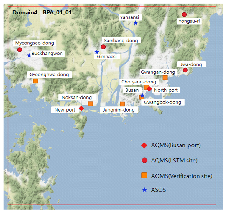
2.1. Study Design
2.2. Input Data
2.3. Method
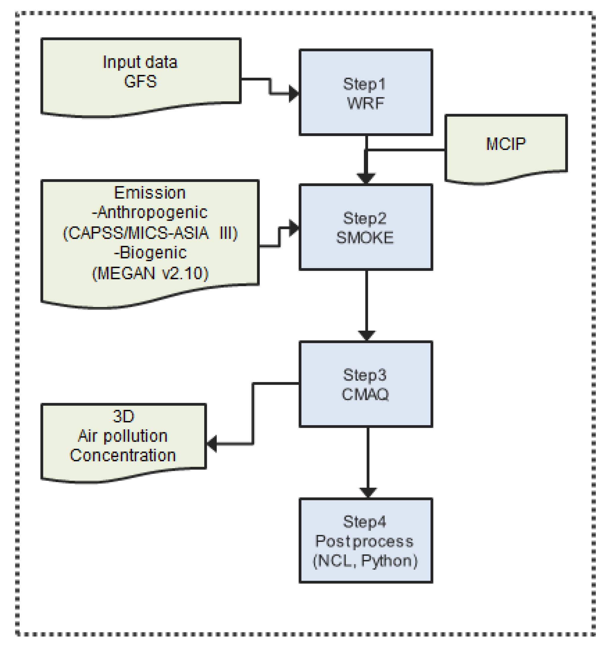
2.3.1. CMAQ
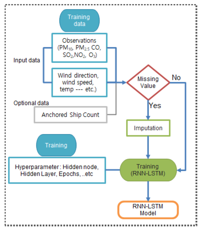
2.3.2. RNN-LSTM
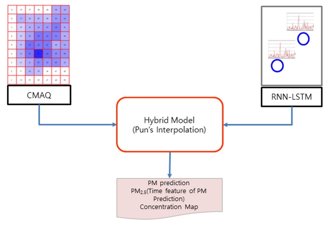
2.3.3. Hybrid (CMAQ and RNN-LSTM) Model
2.3.4. Evaluation Method of Model Performance
3. Results and Discussion
3.1. Result
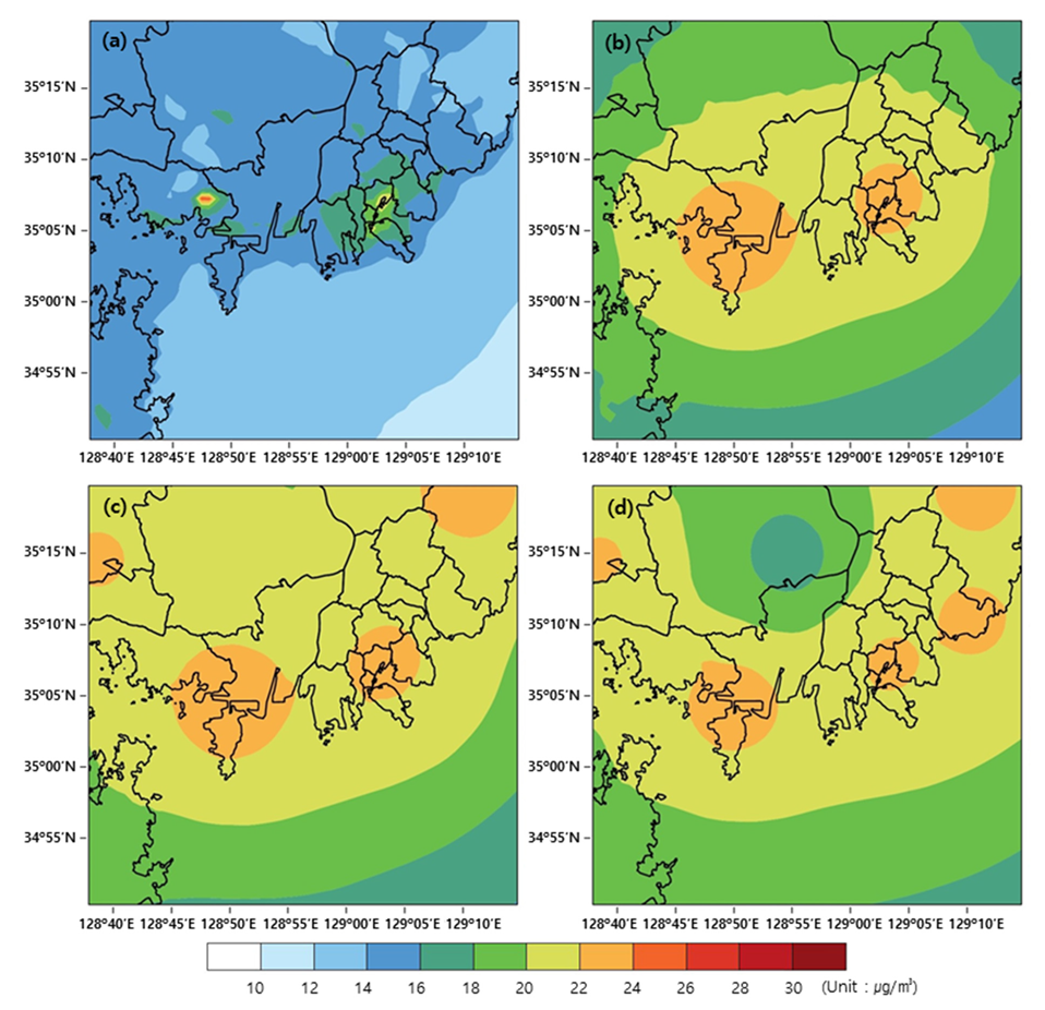
3.1.1. Prediction Results Using the CMAQ Model
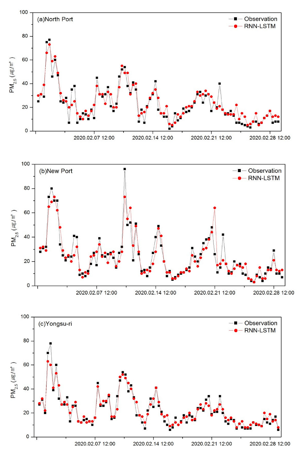
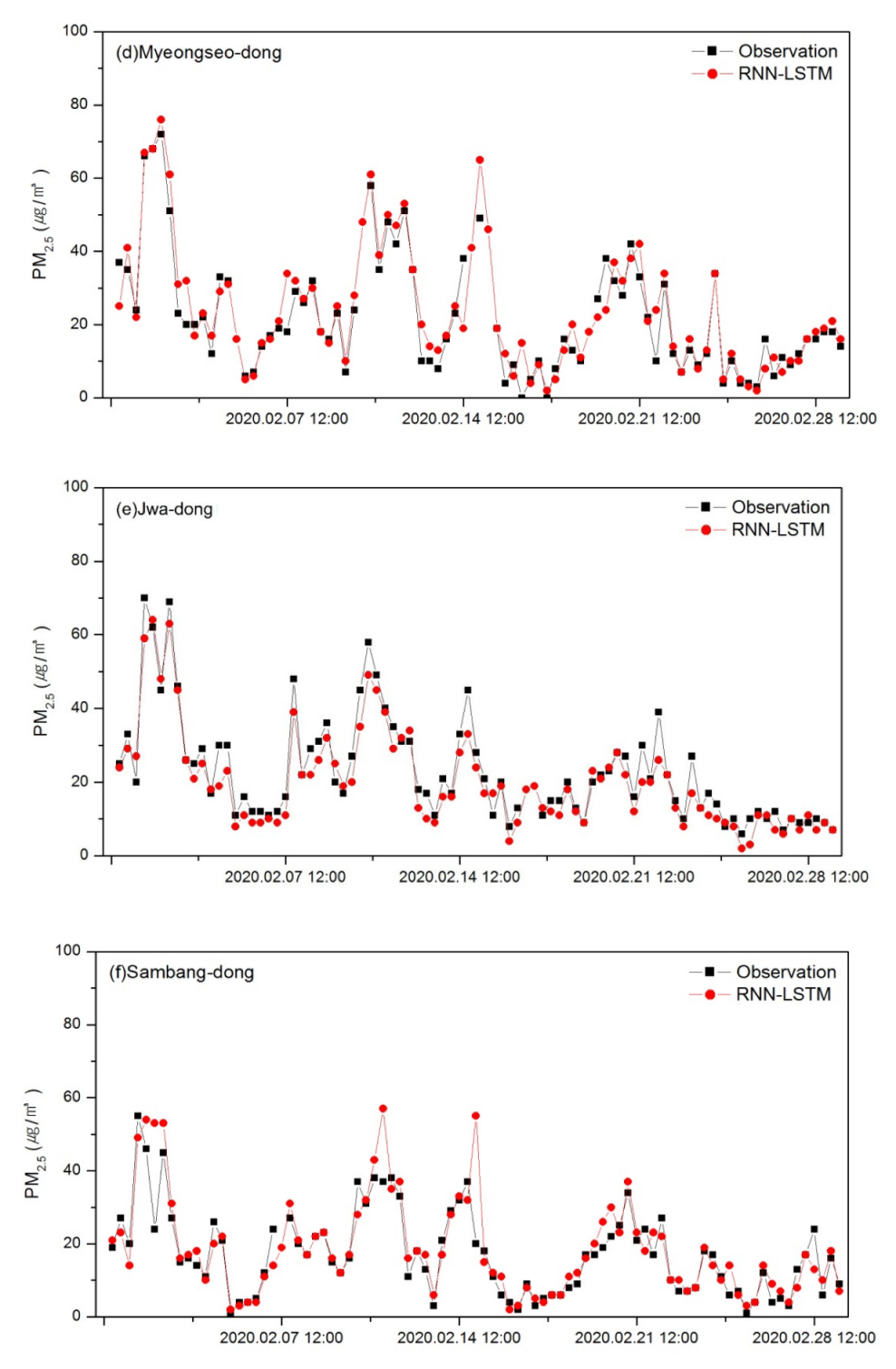
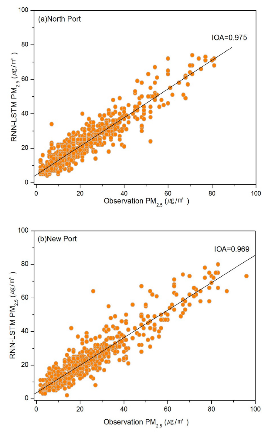
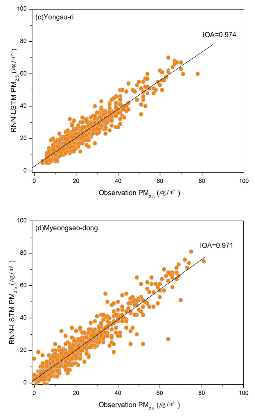
3.1.2. Prediction Results Using the RNN-LSTM Model
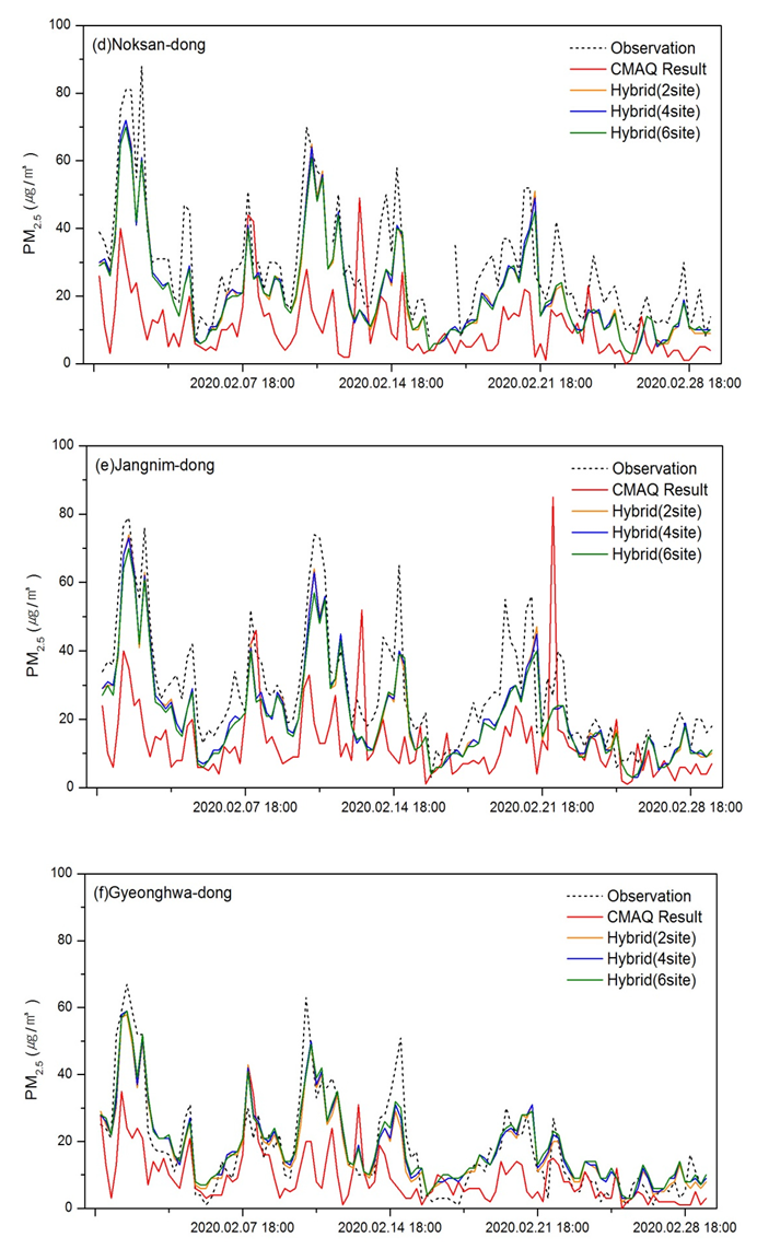
3.1.3. Prediction Results Using the Hybrid Model
3.2. Discussion
4. Conclusions
Author Contributions
Funding
Institutional Review Board Statement
Informed Consent Statement
Data Availability Statement
Acknowledgments
Conflicts of Interest
References
- Murphy, B.N.; Nolte, C.G.; Sidi, F. The detailed emissions scaling, isolation, and diagnostic (DESID) module in the Community Multiscale Air Quality (CMAQ) modeling system version 5.3.2. Geosci. Model Dev. 2021, 14, 3407–3420. [Google Scholar] [CrossRef] [PubMed]
- United States Environmental Protection Agency (USEPA). Integrated Science Assessment for Particulate Matter; United States Environmental Protection Agency: Washington, DC, USA, 2019.
- Bailey, D.; Plenys, T.; Solomon, G.M.; Campbell, T.R.; Feuer, G.R.; Masters, J.; Tonkonogy, B. Harboring Pollution: The Dirty Truth about U.S. Ports; Natural Resources Defense Council: New York, NY, USA, 2004. [Google Scholar]
- Han, C. Air Pollution Reduction Strategies of World Major Ports. Int. Commer. Law Rev. 2010, 48, 27–56. [Google Scholar]
- EPA. Current Methodologies in Preparing Mobile Source Port-Related Emission Inventories; ICF International: Fairfax, VA, USA, 2009.
- Mueller, D.; Uibel, S.; Takemura, M.; Klingelhoefer, D.; Groneberg, D.A. Ships, Ports and Particulate Air Pollution—An Analysis of Recent Studies. J. Occup. Med. Toxicol. 2011, 6, 31. [Google Scholar] [CrossRef] [PubMed]
- Talley, W.K. Port Pollution and Abatement Policies Conference. Available online: https://www.dbpia.co.kr/pdf/pdfView.do?nodeId=NODE01783503&googleIPSandBox=false&mark=0&useDate=&ipRange=false&accessgl=Y&language=ko_KR&hasTopBanner=true (accessed on 15 July 2022).
- Feng, J.; Zhang, Y.; Li, S.; Mao, J.; Patton, A.; Zhou, Y.; Ma, W.; Liu, C.; Kan, H.; Huang, C.; et al. The Influence of Spatiality on Shipping Emissions, Air Quality and Potential Human Exposure in the Yangtze River Delta/Shanghai, China. Atmos. Chem. Phys. 2019, 19, 6167–6183. [Google Scholar] [CrossRef]
- IMO. Guidelines for Consistent Implementation of the 0.50% Sulphur Limit under Marpol; International Marit Organ: London, UK, 2019. [Google Scholar]
- Community Modeling and Analysis System. Developers’ Guide for the Community Multiscale Air Quality (CMAQ) Modeling System; University of North Carolina at Chapel Hill: Chapel Hill, NC, USA, 2019. [Google Scholar]
- Penn, S.L.; Arunachalam, S.; Woody, M.; Heiger-Bernays, W.; Tripodis, Y.; Levy, J.I. Estimating State-Specific Contributions to PM2.5- and O3-Related Health Burden from Residential Combustion and Electricity Generating Unit Emissions in the United States. Environ. Health Perspect. 2017, 125, 324–332. [Google Scholar] [CrossRef]
- Chen, X.; Zhang, Y.; Wang, K.; Tong, D.; Lee, P.; Tang, Y.; Huang, J.; Campbell, P.C.; Mcqueen, J.; Pye, H.O.T.; et al. Evaluation of the Offline-Coupled GFSv15–FV3–CMAQv5.0.2 in Support of the next-Generation National Air Quality Forecast Capability over the Contiguous United States. Geosci. Model Dev. 2021, 14, 3969–3993. [Google Scholar] [CrossRef] [PubMed]
- Russo, A.; Raischel, F.; Lind, P.G. Air Quality Prediction Using Optimal Neural Networks with Stochastic Variables. Atmos. Environ. 2013, 79, 822–830. [Google Scholar] [CrossRef]
- Wu, Z.; Wu, X.; Wang, Y.; He, S. PM2.5/PM10 Ratio Prediction Based on a Long Short-Term Memory Neural Network in Wuhan, China. Geosci. Model Dev. 2020, 13, 1499–1511. [Google Scholar] [CrossRef]
- Li, L.; Chen, B.; Zhang, Y.; Zhao, Y.; Xian, Y.; Xu, G.; Zhang, H.; Guo, L. Retrieval of daily PM2.5 concentrations using nonlinear methods: A case study of the Beijing-Tianjin-Hebei Region, China. Remote Sens. 2018, 10, 2006. [Google Scholar] [CrossRef]
- Chen, Y.-Y.; Lv, Y.; Li, Z.; Wang, F.-Y. Long short-term memory model for traffic congestion prediction with online open data. In Proceedings of the 2016 IEEE 19th International Conference on Intelligent Transportation Systems (ITSC), Rio de Janeiro, Brazil, 1–4 November 2016; pp. 132–137. [Google Scholar]
- Skrobek, D.; Krzywanski, J.; Sosnowski, M.; Kulakowska, A.; Zylka, A.; Grabowska, K.; Ciesielska, K.; Nowak, W. Prediction of Sorption Processes Using the Deep Learning Methods (Long Short-Term Memory). Energies 2020, 13, 6601. [Google Scholar] [CrossRef]
- Binkowski, F.S.; Roselle, S.J. Models-3 Community Multiscale Air Quality (CMAQ) Model Aerosol Component 1. Model Description. J. Geophys. Res. Atmos. 2003, 108, 2001JD001409. [Google Scholar] [CrossRef]
- Mebust, M.R.; Eder, B.K.; Binkowski, F.S.; Roselle, S.J. Models-3 Community Multiscale Air Quality (CMAQ) Model Aerosol Component 2. Model Evaluation. J. Geophys. Res. Atmos. 2003, 108, 2001JD001410. [Google Scholar] [CrossRef]
- Shimadera, H.; Hayami, H.; Chatani, S.; Morikawa, T.; Morino, Y.; Mori, Y.; Yamaji, K.; Nakatsuka, S.; Ohara, T. Urban Air Quality Model Inter-Comparison Study (UMICS) for Improvement of PM2.5 Simulation in Greater Tokyo Area of Japan. Asian J. Atmos. Environ. 2018, 12, 139–152. [Google Scholar] [CrossRef]
- Xayasouk, T.; Lee, H.; Lee, G. Air Pollution Prediction Using Long Short-Term Memory (LSTM) and Deep Autoencoder (DAE) Models. Sustainability 2020, 12, 2570. [Google Scholar] [CrossRef]
- Zhao, J.; Deng, F.; Cai, Y.; Chen, J. Long Short-Term Memory—Fully Connected (LSTM-FC) Neural Network for PM2.5 Concentration Prediction. Chemosphere 2019, 220, 486–492. [Google Scholar] [CrossRef] [PubMed]
- Ma, P.; Tao, F.; Gao, L.; Leng, S.; Yang, K.; Zhou, T. Retrieval of Fine-Grained PM2.5 Spatiotemporal Resolution Based on Multiple Machine Learning Models. Remote Sens. 2022, 14, 599. [Google Scholar] [CrossRef]
- Gao, L.; Tao, F.; Ma, P.; Wang, C.; Kong, W.; Chen, W.; Zhou, T. A short-distance healthy route planning approach. J. Transp. Health 2022, 24, 101314. [Google Scholar] [CrossRef]
- Chen, B.; Song, Z.; Huang, J.; Zhang, P.; Hu, X.; Zhang, X.; Guan, X.; Ge, J.; Zhou, X. Estimation of atmospheric PM10 concentration in China using an interpretable deep learning model and top-of-the-atmosphere reflectance data from China’s new generation geostationary meteorological satellite, FY-4A. J. Geophys. Res. Atmos. 2022, 127, e2021JD036393. [Google Scholar] [CrossRef]
- Song, Z.; Chen, B.; Zhang, P.; Guan, X.; Wang, X.; Ge, J.; Hu, X.; Zhang, X.; Wang, Y. High Temporal and Spatial Resolution PM2.5 Dataset Acquisition and Pollution Assessment Based on FY-4A TOAR Data and Deep Forest Model in China. Atmos. Res. 2022, 274, 106199. [Google Scholar] [CrossRef]
- Kim, H.S.; Park, I.; Song, C.H.; Lee, K.; Yun, J.W.; Kim, H.K.; Jeon, M.; Lee, J.; Han, K.M. Development of a Daily PM10 and PM2.5 Prediction System Using a Deep Long Short-Term Memory Neural Network Model. Atmos. Chem. Phys. 2019, 19, 12935–12951. [Google Scholar] [CrossRef]
- Lee, J.B.; Lee, J.B.; Koo, Y.S.; Kwon, H.Y.; Choi, M.H.; Park, H.J.; Lee, D.G. Development of a Deep Neural Network for Predicting 6 h Average PM2.5 Concentrations up to 2 Subsequent Days Using Various Training Data. Geosci. Model Dev. 2022, 15, 3797–3813. [Google Scholar] [CrossRef]
- Hong, H.; Jeon, H.; Youn, C.; Kim, H.S. Incorporation of Shipping Activity Data in Recurrent Neural Networks and Long Short-Term Memory Models to Improve Air Quality Predictions around Busan Port. Atmosphere 2021, 12, 1172. [Google Scholar] [CrossRef]
- Qi, Y.; Li, Q.; Karimian, H.; Liu, D. A hybrid model for spatiotemporal forecasting of PM2.5 based on graph convolutional neural network and long short-term memory. Sci. Total Environ. 2019, 664, 1–10. [Google Scholar] [CrossRef] [PubMed]
- Pak, U.; Ma, J.; Ryu, U.; Ryom, K.; Juhyok, U.; Pak, K.; Pak, C. Deep learning-based PM2.5 prediction considering the spatiotemporal correlations: A case study of Beijing, China. Sci. Total Environ. 2020, 699, 133561. [Google Scholar] [CrossRef] [PubMed]
- Lu, X.; Sha, Y.; Li, Z.; Huang, Y.; Chen, W.; Chen, D.; Shen, J.; Chen, Y.; Fung, J. Development and application of a hybrid long-short term memory–three dimensional variational technique for the improvement of PM2.5 forecasting. Sci. Total Environ. 2021, 770, 144221. [Google Scholar] [CrossRef]
- Li, X.; Peng, L.; Yao, X.; Cui, S.; Hu, Y.; You, C.; Chi, T. Long short-term memory neural network for air pollutant concentration predictions: Method development and evaluation. Environ. Pollut. 2017, 231, 997–1004. [Google Scholar] [CrossRef]
- Guo, X.; Wang, Y.; Mei, S.; Shi, C.; Liu, Y.; Pan, L.; Li, K.; Zhang, B.; Wang, J.; Zhong, Z.; et al. Monitoring and modelling of PM2.5 concentration at subway station construction based on IoT and LSTM algorithm optimization. J. Clean. Prod. 2022, 360, 132179. [Google Scholar] [CrossRef]
- Isakov, V.; Touma, J.S.; Burke, J.; Lobdell, D.T.; Palma, T.; Rosenbaum, A.; KÖzkaynak, H. Combining Regional- and Local-Scale Air Quality Models with Exposure Models for Use in Environmental Health Studies. J. Air Waste Manage. Assoc. 2009, 59, 461–472. [Google Scholar] [CrossRef]
- Oh, I.; Hwang, M.-K.; Bang, J.-H.; Yang, W.; Kim, S.; Lee, K.; Seo, S.; Lee, J.; Kim, Y. Comparison of Different Hybrid Modeling Methods to Estimate Intraurban NO2 Concentrations. Atmos. Environ. 2021, 244, 117907. [Google Scholar] [CrossRef]
- Community Modeling and Analysis System. Operational Guidance for the Community Multiscale Air Quality (CMAQ) Modeling System; University of North Carolina at Chapel Hill: Chapel Hill, NC, USA, 2010. [Google Scholar]
- Reddy, V.; Yedavalli, P.; Mohanty, S.; Nakhat, U. Deep Air: Forecasting Air Pollution in Beijing, China. 2017. Available online: https://www.ischool.berkeley.edu/sites/default/files/sproject_attachments/deep-air-forecasting_final.pdf (accessed on 23 August 2022).
- Akima, H. A New Method of Interpolation and Smooth Curve Fitting. J. ACM 1970, 17, 589–602. [Google Scholar] [CrossRef]
- Hochreiter, S. Long Short-Term Memory. Neural Comput. 1997, 1780, 1735–1780. [Google Scholar] [CrossRef] [PubMed]
- Zhang, Y.; Vijayaraghavan, K.; Wen, X.Y.; Snell, H.E.; Jacobson, M.Z. Probing into Regional Ozone and Particulate Matter Pollution in the United States: 1. A 1 Year CMAQ Simulation and Evaluation Using Surface and Satellite Data. J. Geophys. Res. Atmos. 2009, 114, D22304. [Google Scholar] [CrossRef]
- Pun, B.K.; Seigneur, C. Using Cmaq To Interpolate Among Castnet Measurements. In Proceedings of the CMAS Conference, San Ramon, CA, USA, 18 October 2006; pp. 1–6. [Google Scholar]
- Chang, L.; Scorgie, Y.; Duc, H.; Monk, K.; Fuchs, D.; Trieu, T. Major Source Contributions to Ambient PM2.5 and Exposures within the New South Wales Greater Metropolitan Region. Atmosphere 2019, 10, 138. [Google Scholar] [CrossRef] [Green Version]
- Tesche, T.W.; McNally, D.E. Operational Evaluation of the MM5 Meteorological Model over the Continental United States: Protocol for Annual and Episodic Evaluation Task Order 4TCG-68027015; Alpine Geophysics, LLC: Ft. Wright, KY, USA, 2002. [Google Scholar]
- Emery, C.; Tai, E.; Yarwood, G. Enhanced Meteorological Modeling and Performance Evaluation for Two Texas Ozone Episodes; ENVIRON, International Corp.: Novato, CA, USA, 2001. [Google Scholar]


| Description | ||||
|---|---|---|---|---|
| Projection origin | 126° E, 38° N | |||
| Projection | Lambert conformal conic | |||
| Two standard parallels of latitude of projection origin | 30°, 60° | |||
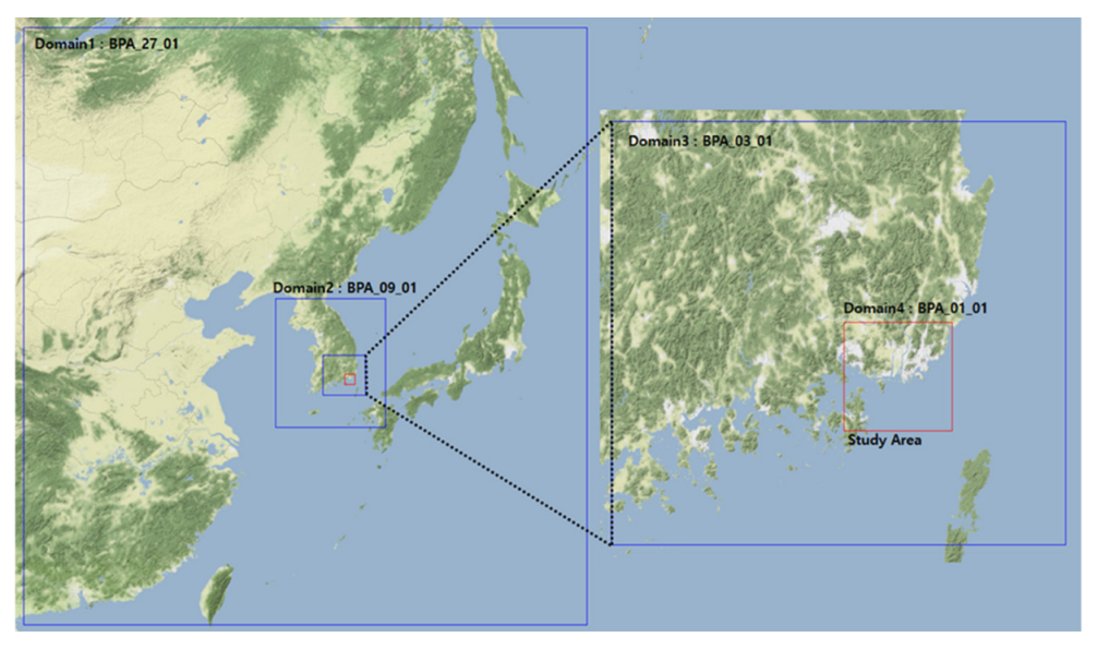
| Domain name | BPA_27_01 | BPA_09_01 | BPA_03_01 | BPA_01_01 |
| Horizontal resolution (Size and Count) | 27 km | 9 km | 3 km | 1 km |
| 121 × 128 | 70 × 82 | 82 × 76 | 58 × 58 | |
| X-origin | −1,633,500 m | −166,500 m | 106,500 m | 233,500 m |
| Y-origin | −1,728,000 m | −585,000 m | −402,000 m | −341,000 m |
| Model | Input Data | Output Data | |
|---|---|---|---|
| CMAQ | Meteorological | NCEP GFS 0.25 Degree Global Forecast data | Gridded Concentration (PM2.5, PM10, O3, etc.) |
| Emission | PM2.5, PM10 O3, NO2, SO2, CO | ||
| RNN-LSTM | Surface Meteorological | Temperature, Dew point Pressure Wind speed Wind Direction Rainfall | PM2.5 |
| Air quality | PM2.5, PM10 O3, NO2, SO2, CO | ||
| Emission activity | Anchored ships | ||
| Hybrid Model | Gridded Concentration (PM2.5, PM10, O3, etc.) of the CMAQ result | Gridded Concentration (PM2.5) | |
| PM2.5 of RNN-LSTRM result | |||
| Type | Input Parameters | Timing | Unit |
|---|---|---|---|
| Air quality data | PM2.5, PM10 | every 1-h | µg/m3 |
| SO2, O3, NO2, CO | every 1-h | ppm | |
| Meteorological data | Temperature | every 1-h | °C |
| Dew point | every 1-h | °C | |
| Pressure | every 1-h | hPa | |
| Wind speed | every 1-h | m/s | |
| Wind Direction | every 1-h | Degree | |
| Rainfall | every 1-h | mm | |
| Shipping activity Data | anchored ships | every 1-h | ea |
| Type | Condition Values | Applied Values |
|---|---|---|
| Optimizer | Adam, Adamax, RMSprop | Adam |
| Batch size | 50, 100, 200 | 100 |
| Learning rate | 0.001, 0.01, 0.1 | 0.001 |
| Dropout | 0.2, 0.3, 0.4 | 0.2 |
| Loss function | Loss, L2 Loss, L1 Loss | L2 Loss |
| Type | Configuration | Settings |
|---|---|---|
| Data partition | Training set | 8760 |
| Validation set | 744 | |
| Test set | 696 |
| Site | Input Data | Hyperparameter |
|---|---|---|
| North Port | AQMS 1 + ASOS 2 (Busan) + Anchored Ships Information | Hidden nodes: 30, 60, 120 Hidden Layers: 1, 2, 3 Epochs: 10, 15, 20 |
| New Port | ||
| Yongsu-ri | AQMS + ASOS (Yangsansi) | |
| Myeongseo-dong | AQMS + ASOS (Bukchangwon) | |
| Jwa-dong | AQMS + ASOS (Busan) | |
| Sambang-dong | AQMS + ASOS (Gimhaesi) |
| Site | OBS Mean | Model Mean | NMB | MNGE | RMSE | IOA |
|---|---|---|---|---|---|---|
| North Port | 21.8 | 19.0 | −13.1 | 56.68 | 13.63 | 0.684 |
| New Port | 23.1 | 17.5 | −24.1 | 52.97 | 16.10 | 0.612 |
| Yongsu-ri | 22.7 | 17.5 | −22.9 | 35.41 | 12.26 | 0.663 |
| Myeongseo-dong | 22.2 | 16.0 | −28.0 | 62.23 | 15.04 | 0.616 |
| Jwa-dong | 23.1 | 18.8 | −18.7 | 41.33 | 14.62 | 0.600 |
| Sambang-dong | 17.5 | 17.3 | −1.4 | 98.3 | 11.86 | 0.646 |
| Site Name | Optimal Training Parameters | NMB (%) | MNGE (%) | RMSE (μg/m3) | IOA | ||
|---|---|---|---|---|---|---|---|
| Hidden Node | Hidden Layer | Epochs | |||||
| (a) North Port | 120 | 1 | 15 | 2.8 | 24.28 | 4.88 | 0.975 |
| (b) New Port | 120 | 1 | 20 | −3.5 | 23.79 | 5.87 | 0.969 |
| (c) Yongsu-ri | 60 | 1 | 20 | 0.9 | 17.38 | 4.12 | 0.974 |
| (d) Myeongseo-dong | 120 | 1 | 20 | 1.1 | 26.39 | 5.39 | 0.971 |
| (e) Jwa-dong | 60 | 1 | 20 | −2.1 | 16.69 | 4.26 | 0.974 |
| (f) Sambang-dong | 30 | 1 | 20 | −0.7 | 28.01 | 5.07 | 0.961 |
| Port | Verification Site | Latitude | Longitude | Distance from Busan Port (km) |
|---|---|---|---|---|
| North Port | Choryang-dong | 35.12714 | 129.0467 | 0.90 |
| Gwangbok-dong | 35.09985 | 129.0303 | 3.35 | |
| Gwangan-dong | 35.15231 | 129.1081 | 5.71 | |
| New Port | Noksan-dong | 35.08663 | 128.8639 | 2.95 |
| Jangnim-dong | 35.08298 | 128.9668 | 11.90 | |
| Gyeonghwa-dong | 35.15497 | 128.6896 | 15.61 |
| Site | Type | OBS Mean (μg/m3) | Model Mean (μg/m3) | NMB (%) | MNGE (%) | RMSE (μg/m3) | IOA |
|---|---|---|---|---|---|---|---|
| (a) Choryang-dong | CMAQ | 21.1 | 19.3 | −8.4 | 55.89 | 13.56 | 0.684 |
| Hybrid (2 sites) | 21.8 | 3.7 | 27.03 | 5.31 | 0.967 | ||
| Hybrid (4 sites) | 21.9 | 4.2 | 27.08 | 5.18 | 0.968 | ||
| Hybrid (6 sites) | 18.8 | −10.3 | 25.2 | 6.08 | 0.947 | ||
| (b) Gwangbok-dong | CMAQ | 19.4 | 19.4 | 0.9 | 83.16 | 12.27 | 0.683 |
| Hybrid (2 sites) | 21.7 | 13.3 | 44.16 | 6.81 | 0.940 | ||
| Hybrid (4 sites) | 21.8 | 13.9 | 44.82 | 6.66 | 0.942 | ||
| Hybrid (6 sites) | 20.7 | 8.1 | 41.06 | 5.99 | 0.949 | ||
| (c) Gwangan-dong | CMAQ | 22.5 | 19.5 | −13.6 | 43.64 | 13.3 | 0.683 |
| Hybrid (2 sites) | 21.2 | −5.7 | 24.00 | 5.29 | 0.966 | ||
| Hybrid (4 sites) | 21.6 | −4.1 | 22.19 | 4.88 | 0.970 | ||
| Hybrid (6 sites) | 20.6 | −8.4 | 21.04 | 5.11 | 0.965 | ||
| (d) Noksan-dong | CMAQ | 29.4 | 17.8 | −39.1 | 40.19 | 19.28 | 0.590 |
| Hybrid (2 sites) | 21.5 | −25.6 | 28.84 | 10.87 | 0.895 | ||
| Hybrid (4 sites) | 21.6 | −25.3 | 28.104 | 10.78 | 0.895 | ||
| Hybrid (6 sites) | 21.7 | −26.3 | 28.33 | 11.00 | 0.888 | ||
| (e) Jangnim-dong | CMAQ | 28.7 | 19.9 | −30.4 | 41.80 | 17.79 | 0.600 |
| Hybrid (2 sites) | 21.9 | −23.2 | 28.13 | 9.35 | 0.917 | ||
| Hybrid (4 sites) | 22.0 | −23.0 | 27.56 | 9.31 | 0.917 | ||
| Hybrid (6 sites) | 21.3 | −25.4 | 28.72 | 9.81 | 0.905 | ||
| (f) Gyeonghwa-dong | CMAQ | 18.2 | 16.4 | −9.7 | 111.86 | 12.56 | 0.680 |
| Hybrid (2 sites) | 17.7 | −2.4 | 64.23 | 7.74 | 0.915 | ||
| Hybrid (4 sites) | 18.4 | 1.5 | 66.12 | 7.33 | 0.925 | ||
| Hybrid (6 sites) | 18.8 | 3.8 | 68.27 | 7.17 | 0.928 |
Publisher’s Note: MDPI stays neutral with regard to jurisdictional claims in published maps and institutional affiliations. |
© 2022 by the authors. Licensee MDPI, Basel, Switzerland. This article is an open access article distributed under the terms and conditions of the Creative Commons Attribution (CC BY) license (https://creativecommons.org/licenses/by/4.0/).
Share and Cite
Hong, H.; Choi, I.; Jeon, H.; Kim, Y.; Lee, J.-B.; Park, C.H.; Kim, H.S. An Air Pollutants Prediction Method Integrating Numerical Models and Artificial Intelligence Models Targeting the Area around Busan Port in Korea. Atmosphere 2022, 13, 1462. https://doi.org/10.3390/atmos13091462
Hong H, Choi I, Jeon H, Kim Y, Lee J-B, Park CH, Kim HS. An Air Pollutants Prediction Method Integrating Numerical Models and Artificial Intelligence Models Targeting the Area around Busan Port in Korea. Atmosphere. 2022; 13(9):1462. https://doi.org/10.3390/atmos13091462
Chicago/Turabian StyleHong, Hyunsu, IlHwan Choi, Hyungjin Jeon, Yumi Kim, Jae-Bum Lee, Cheong Hee Park, and Hyeon Soo Kim. 2022. "An Air Pollutants Prediction Method Integrating Numerical Models and Artificial Intelligence Models Targeting the Area around Busan Port in Korea" Atmosphere 13, no. 9: 1462. https://doi.org/10.3390/atmos13091462
APA StyleHong, H., Choi, I., Jeon, H., Kim, Y., Lee, J.-B., Park, C. H., & Kim, H. S. (2022). An Air Pollutants Prediction Method Integrating Numerical Models and Artificial Intelligence Models Targeting the Area around Busan Port in Korea. Atmosphere, 13(9), 1462. https://doi.org/10.3390/atmos13091462