

Future Projections of Extreme Precipitation Climate Indices over South America Based on CORDEX-CORE Multimodel Ensemble

 , ,
, ,
Abstract
1. Introduction
2. Materials and Methods
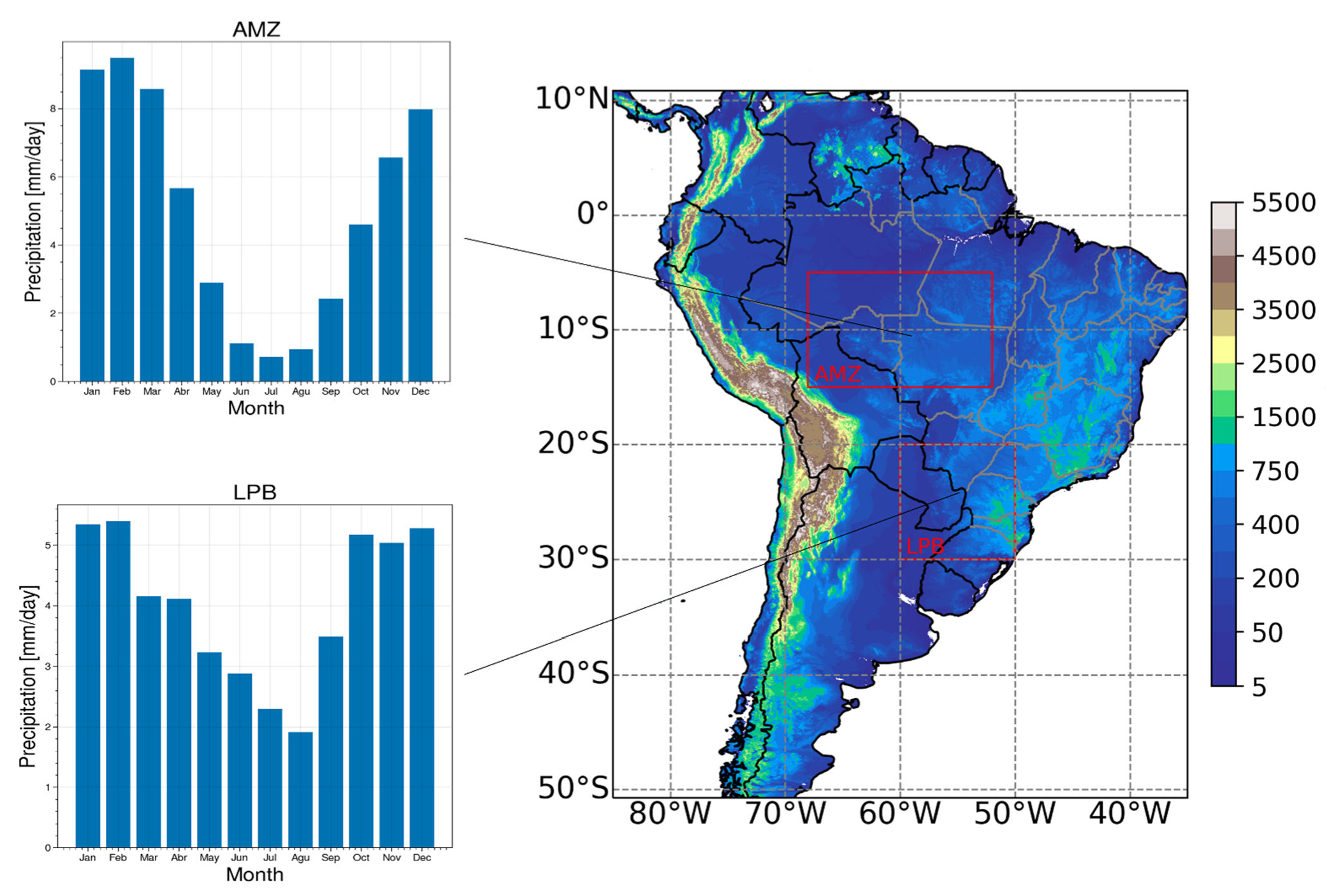
2.1. Study Area
2.2. Data
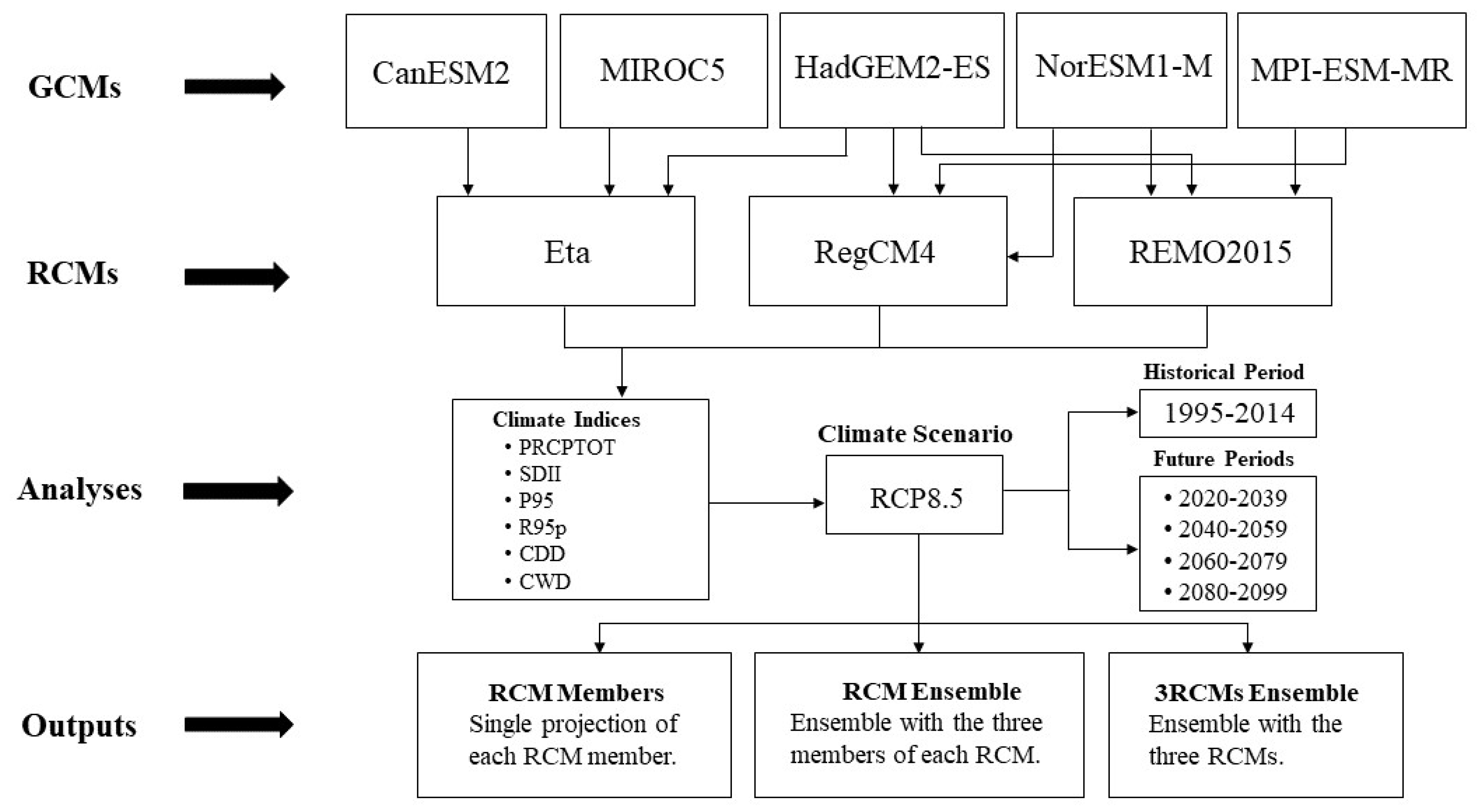
2.3. RCM Projections

| RCM | Horizontal Resolution and Reference | GCM | GCM Resolution | References |
|---|---|---|---|---|
| Eta | 0.20° × 0.20° Mesinger et al. [52] Chou et al. [17] | CanESM2 | 2.7906° × 2.8125° | Chylek et al. [53] Arora et al. [54] |
| HadGEM2-ES | 1.25° × 1.875° | Collins et al. [55] Martin et al. [56] | ||
| MIROC5 | 1.4008° × 1.40625° | Watanabe et al. [57] | ||
| RegCM4 | 0.22° × 0.22° Giorgi et al. [14] | HadGEM2-ES | 1.25° × 1.85° | Collins et al. [55] Martin et al. [56] |
| NorESM1-M | 1.8947° × 2.5° | Bentsen et al. [58] | ||
| MPI-ESM-MR | 1.8653° × 1.875° | Stevens et al. [59] | ||
| REMO2015 | 0.22° × 0.22° Jacob et al. [60] Remedio et al. [16] | HadGEM2-ES | 1.25° × 1.875° | Collins et al. [55] Martin et al. [56] |
| NorESM1-M | 1.8947° × 2.5° | Bentsen et al. [58] | ||
| MPI-ESM-LR | 1.8653° × 1.875° | Stevens et al. [59] |
2.4. Climate Indices
2.5. Analyses
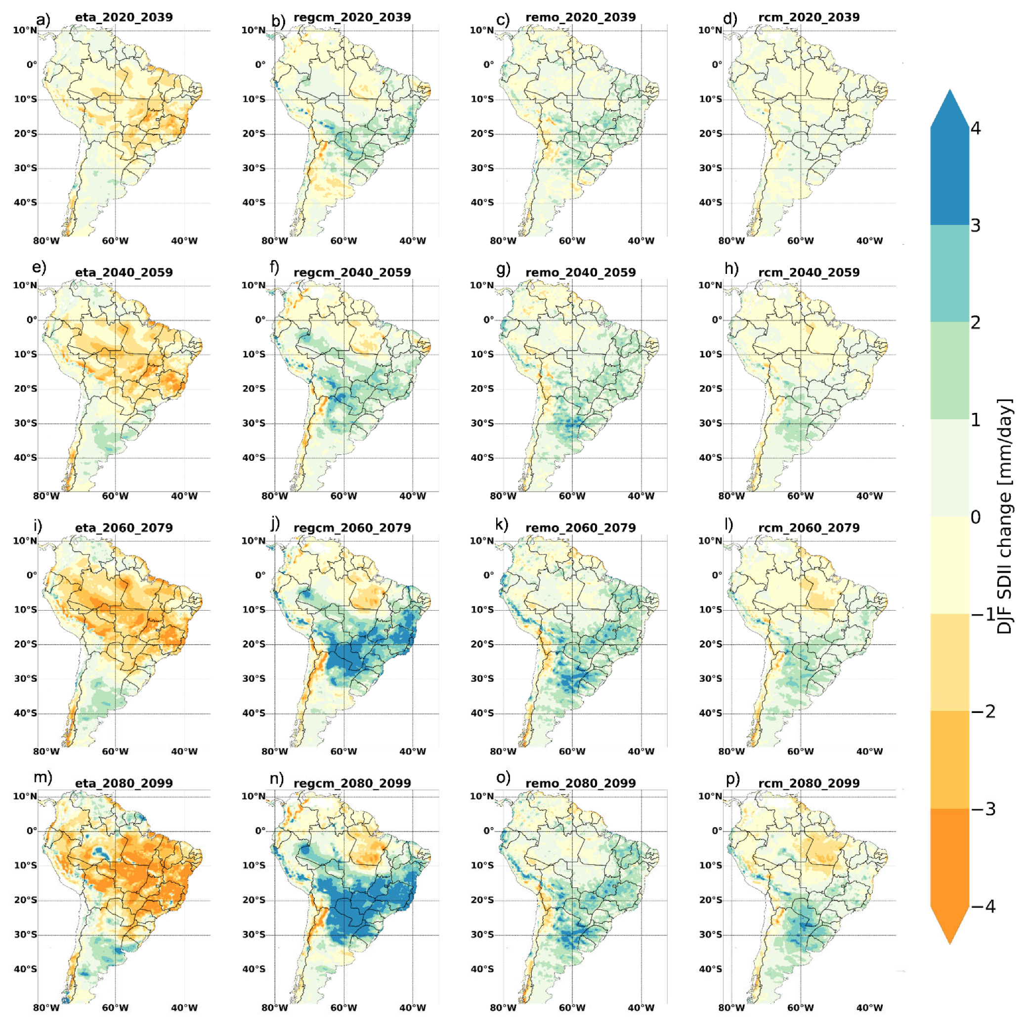
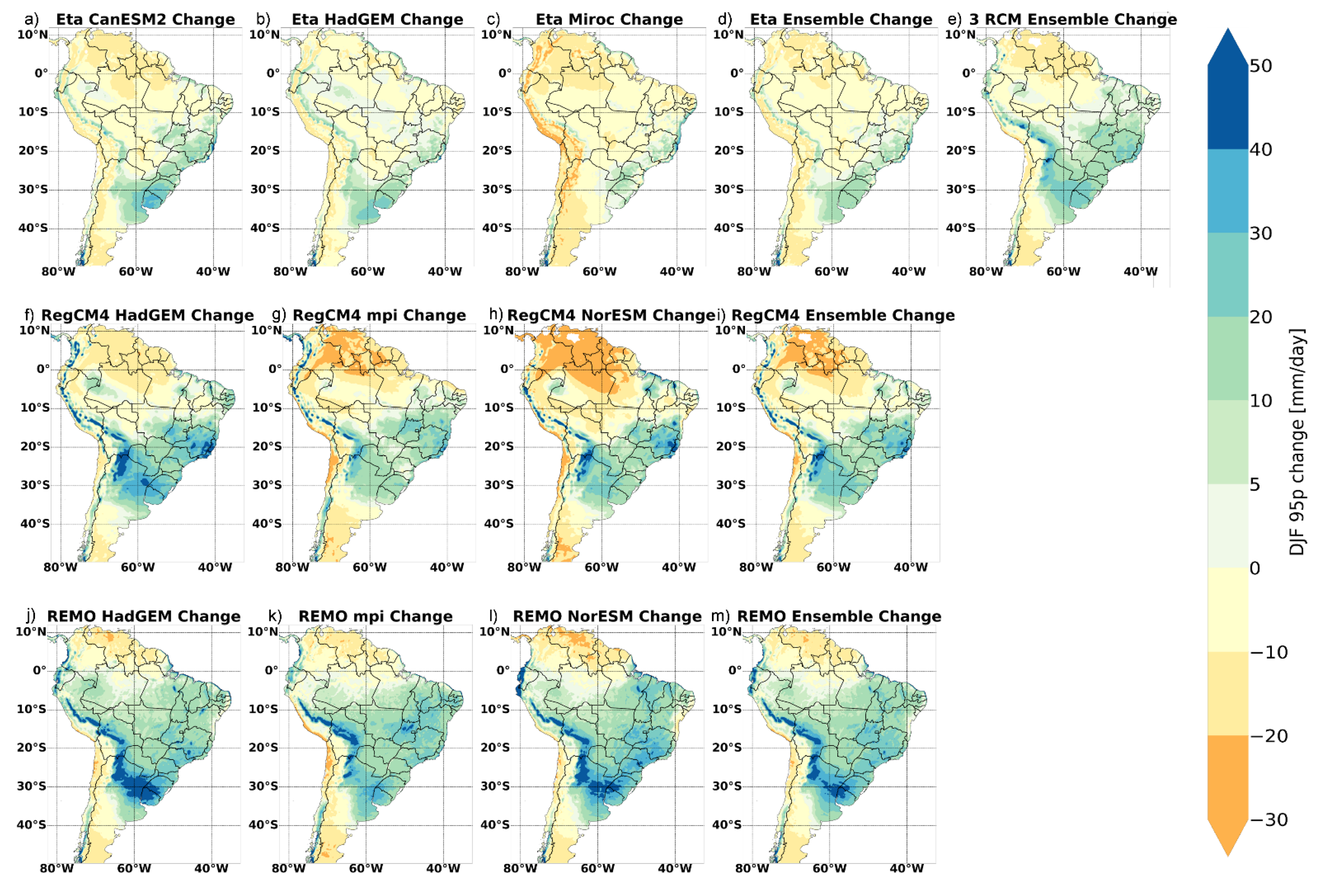
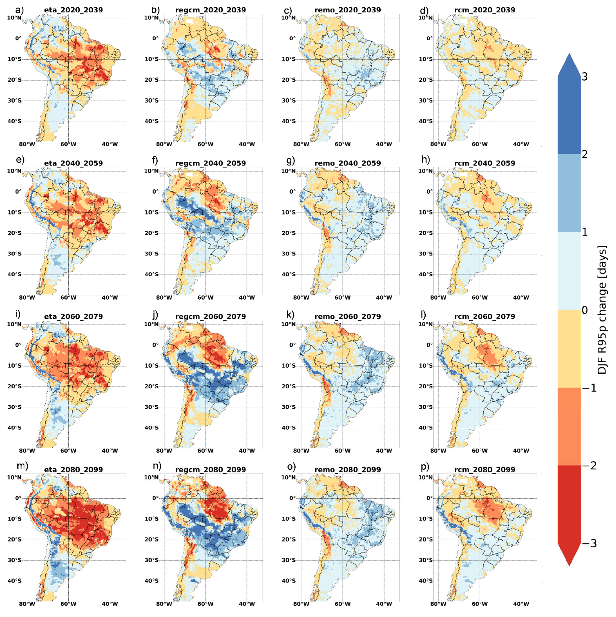
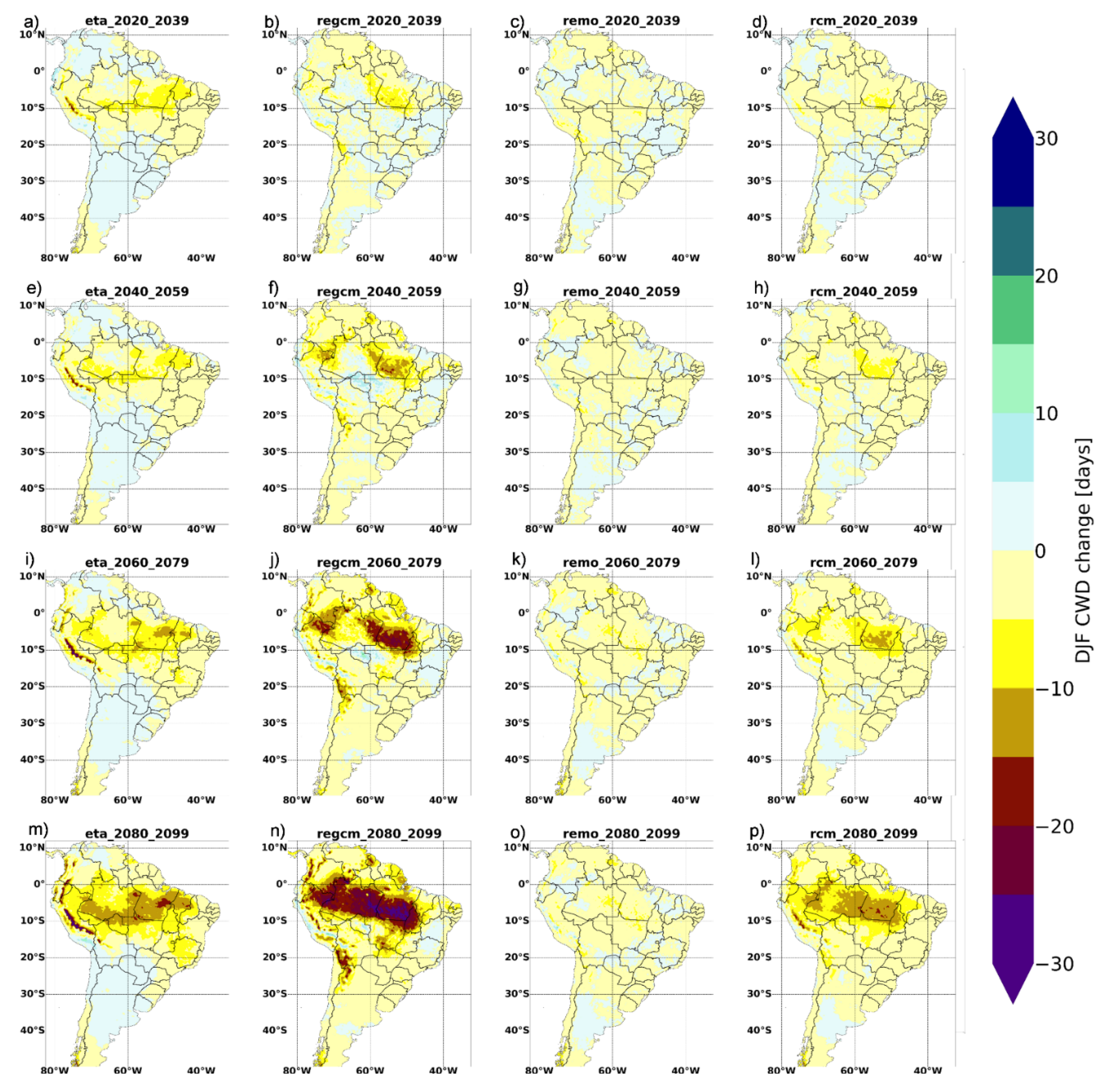
3. Results and Discussion
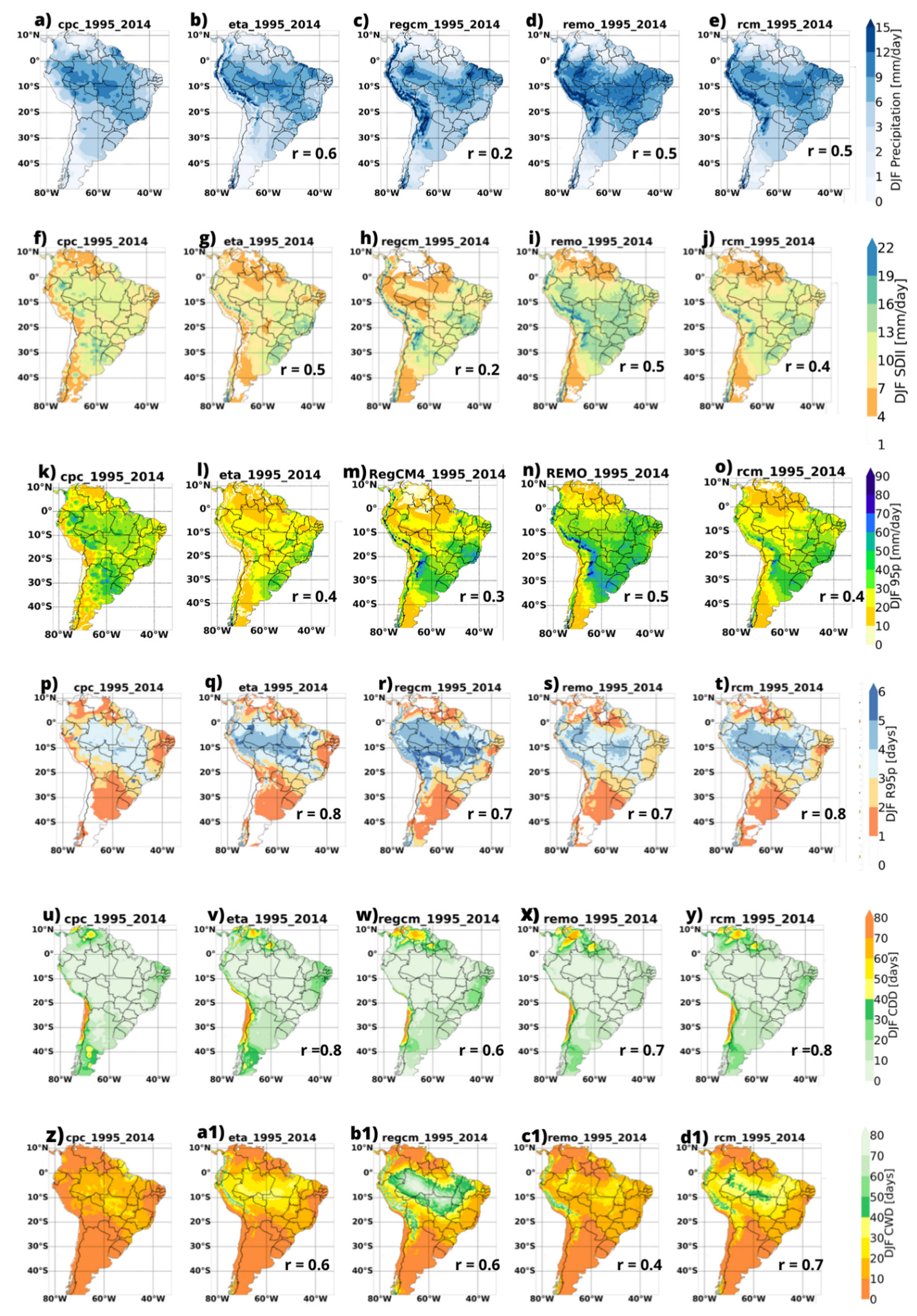
3.1. Present Climate
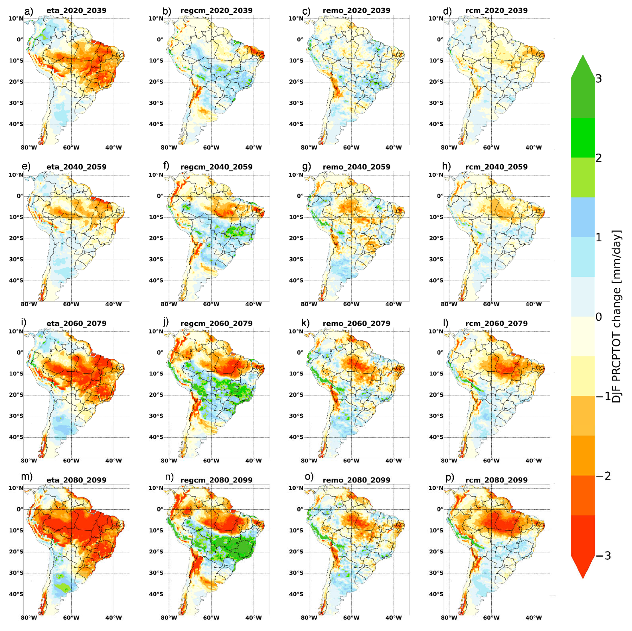
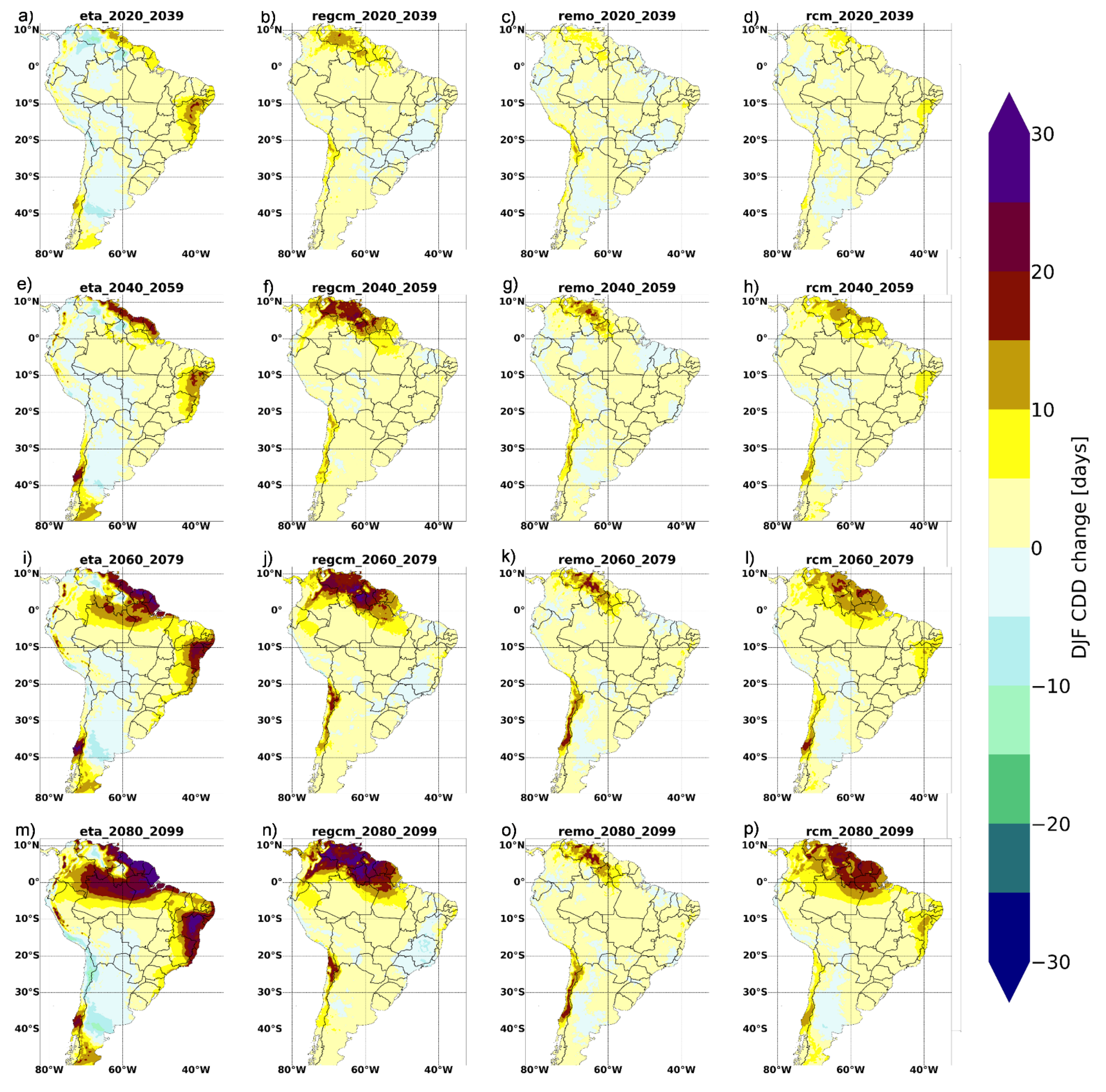
3.2. Future Climate—Spatial Pattern of the Projected Changes
3.3. Trends
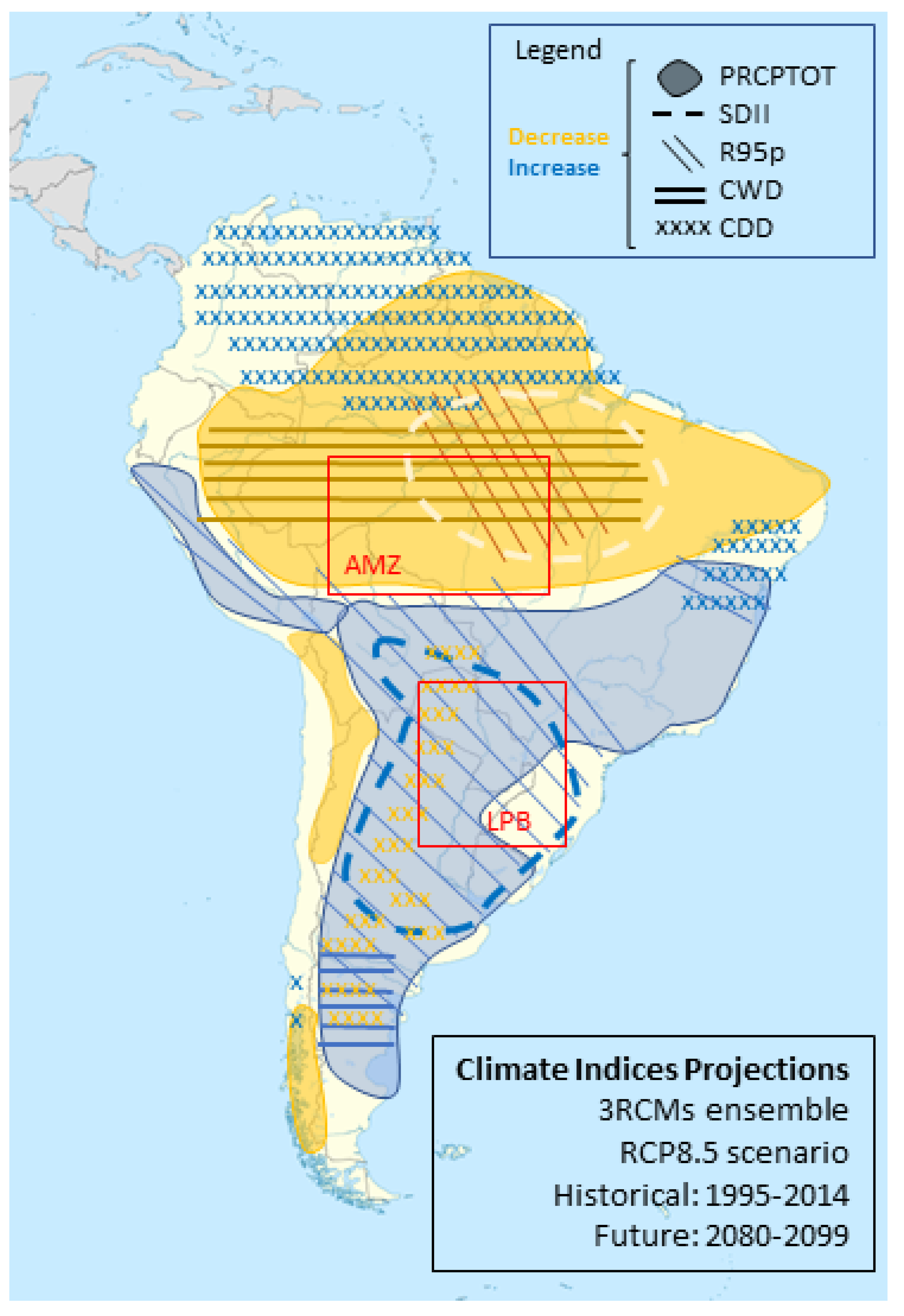
4. Conclusions
- -
- Extreme north of South America: the decrease in PRCPTOT is accomplished by an increase in CDD periods;
- -
- Western Amazon: the decrease in PRCPTOT is accomplished by a decrease in CWD periods;
- -
- Eastern Amazon (north Brazil): the decrease in PRCPTOT is accomplished by a decrease in SDII, CWD, and R95p;
- -
- Semi-arid Brazil (northeast of South America): it is located in a transition region in PRCPTOT and is dominated by an increase in CDD; the southern of this area also shows an increase of R95p;
- -
- La Plata basin (a region that coincides with the dashed line in Figure 11): the increase in PRCPTOT, SDII, and R95p coincides with a decrease in CDD;
- -
- Southern Argentina: the increase in PRCPTOT and R95p occurs concomitantly with a decrease in CDD.
Author Contributions
Funding
Institutional Review Board Statement
Informed Consent Statement
Data Availability Statement
Acknowledgments
Conflicts of Interest
References
- IPCC. Climate change 2014: Synthesis report. In Contribution of Working Groups I, II and III to the Fifth Assessment Report of the Intergovernmental Panel on Climate Change; Pachauri, R.K., Meyer, L.A., Eds.; IPCC: Geneva, Switzerland, 2014; Available online: https://www.ipcc.ch/report/ar5/syr/ (accessed on 15 July 2022).
- IPCC. Climate change 2021: The physical science basis. In Contribution of Working Group I to the Sixth Assessment Report of the Intergovernmental Panel on Climate Change; Masson-Delmotte, V., Zhai, P., Pirani, A., Connors, S.L., Péan, C., Chen, Y., Goldfarb, L., Gomis, M.I., Matthews, J.B.R., Berger, S., et al., Eds.; Cambridge University Press: Cambridge, UK, 2021; Available online: https://www.ipcc.ch/report/ar6/wg1/#FullReport (accessed on 15 July 2022).
- Zilli, M.T.; Carvalho, L.M.V.; Liebmann, B.; Silva Dias, M.A. A comprehensive analysis of trends in extreme precipitation over southeastern coast of Brazil. Int. J. Climatol. 2017, 37, 2269–2279. [Google Scholar] [CrossRef]
- Ruddiman, W.F. Earth’s Climate: Past and Future; W.H. Freeman & Company: New York, NY, USA, 2008. [Google Scholar]
- Trenberth, K. More knowledge, less certainty. Nat. Rep. Clim. Chang. 2010, 1, 20–21. [Google Scholar] [CrossRef]
- Nearing, G.S.; Tian, Y.; Gupta, H.V.; Clark, M.P.; Harrison, K.W.; Weijs, S.V. A philosophical basis for hydrological uncertainty. Hydrol. Sci. J. 2016, 61, 1666–1678. [Google Scholar] [CrossRef]
- Kundzewicz, Z.W.; Krysanova, V.; Benestad, R.E.; Hov, Ø.; Piniewski, M.; Otto, I.M. Uncertainty in climate change impacts on water resources. Environ. Sci. Policy 2018, 79, 1–8. [Google Scholar] [CrossRef]
- Folke, C.; Polasky, S.; Rockström, J.; Galaz, V.; Westley, F.; Lamont, M.; Scheffer, M.; Österblom, H.; Carpenter, S.R.; Chapin, F.S.; et al. Our future in the Anthropocene biosphere. Ambio 2021, 50, 834–869. [Google Scholar] [CrossRef]
- Ambrizzi, T.; Reboita, M.S.; da Rocha, R.P.; Llopart, M. The state of the art and fundamental aspects of regional climate modeling in South America. Ann. N. Y. Acad. Sci. 2019, 1436, 98–120. [Google Scholar] [CrossRef]
- Eyring, V.; Bony, S.; Meehl, G.A.; Senior, C.A.; Stevens, B.; Stouffer, R.J.; Taylor, K.E. Overview of the Coupled Model Intercomparison Project Phase 6 (CMIP6) experimental design and organization. Geosci. Mod. Dev. 2016, 9, 1937–1958. [Google Scholar] [CrossRef]
- Giorgi, F.; Jones, C.; Asrar, G. Addressing climate information needs at the regional level: The CORDEX framework. WMO Bull. 2009, 58, 175–183. Available online: https://public.wmo.int/en/bulletin/addressing-climate-information-needs-regional-level-cordex-framework (accessed on 1 July 2022).
- CORDEX CORE Simulations—CORDEX Coordinated Output for Regional Evaluations (CORE). Available online: https://cordex.org/experiment-guidelines/cordex-core/cordex-core-simulations/ (accessed on 8 August 2022).
- Giorgi, F. Introduction to the special issue: The phase I CORDEX RegCM4 hyper-matrix (CREMA) experiment. Clim. Chang. 2014, 125, 1–5. [Google Scholar] [CrossRef]
- Giorgi, F.; Coppola, E.; Teichmann, C.; Jacob, D. Editorial for the CORDEX-CORE experiment I special issue. Clim. Dyn. 2021, 57, 1265–1268. [Google Scholar] [CrossRef]
- Giorgi, F.; Coppola, E.; Solmon, F.; Mariotti, L.; Sylla, M.B.; Bi, X.; Branković, C. RegCM4: Model description and preliminary tests over multiple CORDEX domains. Clim. Res. 2012, 52, 7–29. [Google Scholar] [CrossRef]
- Remedio, A.R.; Teichmann, C.; Buntemeyer, L.; Sieck, K.; Weber, T.; Rechid, D.; Hoffmann, P.; Nam, C.; Kotova, L.; Jacob, D. Evaluation of new CORDEX simulations using an updated Köeppen–Trewartha climate classification. Atmosphere 2019, 10, 726. [Google Scholar] [CrossRef]
- Chou, S.C.; Lyra, A.; Mourão, C.; Dereczynski, C.; Pilotto, I.; Gomes, J.; Chagas, D. Evaluation of the Eta simulations nested in three global climate models. Am. J. Clim. Chang. 2014, 3, 438. [Google Scholar] [CrossRef]
- Giorgi, F.; Coppola, E.; Raffaele, F.; Diro, G.T.; Fuentes-Franco, R.; Giuliani, G.; Mamgain, A.; Llopart, M.; Mariotti, L.; Torma, C. Changes in extremes and hydroclimatic regimes in the CREMA ensemble projections. Clim. Chang. 2014, 125, 39–51. [Google Scholar] [CrossRef]
- Reboita, M.S.; da Rocha, R.P.; Dias, C.G.; Ynoue, R.Y. Climate projections for South America: RegCM3 driven by HadCM3 and ECHAM5. Adv. Meteorol. 2014, 2014, 376738. [Google Scholar] [CrossRef]
- Reboita, M.S.; Kuki, C.A.C.; Marrafon, V.H.; de Souza, C.A.; Ferreira, G.W.S.; Teodoro, T.A.; Lima, J.W.M. South America climate change revealed through climate indices projected by GCMs and Eta-RCM ensembles. Clim. Dyn. 2022, 58, 459–485. [Google Scholar] [CrossRef]
- Dereczynski, C.; Chou, S.C.; Lyra, A.; Sondermann, M.; Regoto, P.; Tavares, P.; Skansi, M.M. Downscaling of climate extremes over South America—Part I: Model evaluation in the reference climate. Weather Clim. Extrem. 2020, 29, 100273. [Google Scholar] [CrossRef]
- Teodoro, T.A.; Reboita, M.S.; Llopart, M.; da Rocha, R.P.; Ashfaq, M. Climate change impacts on the South American monsoon system and its surface–atmosphere processes through RegCM4 CORDEX-CORE projections. Earth Syst. Environ. 2021, 5, 825–847. [Google Scholar] [CrossRef]
- Falco, M.; Carril, A.F.; Menéndez, C.G.; Zaninelli, P.G.; Li, L.Z. Assessment of CORDEX simulations over South America: Added value on seasonal climatology and resolution considerations. Clim. Dyn. 2019, 52, 4771–4786. [Google Scholar] [CrossRef]
- Solman, A.; Blázquez, J. Multiscale precipitation variability over South America: Analysis of the added value of CORDEX RCM simulations. Clim. Dyn. 2019, 53, 1547–1565. [Google Scholar] [CrossRef]
- Llopart, M.; Reboita, M.S.; da Rocha, R.P. Assessment of multimodel climate projections of water resources over South America CORDEX domain. Clim. Dyn. 2020, 54, 99–116. [Google Scholar] [CrossRef]
- Spinoni, J.; Barbosa, P.; Bucchignani, E.; Cassano, J.; Cavazos, T.; Christensen, J.H.; Christensen, O.B.; Coppola, E.; Evans, J.; Geyer, B.; et al. Future global meteorological drought hot spots: A study based on CORDEX data. J. Clim. 2020, 33, 3635–3661. [Google Scholar] [CrossRef]
- Olmo, M.E.; Bettolli, M.L. Extreme daily precipitation in southern South America: Statistical characterization and circulation types using observational datasets and regional climate models. Clim. Dyn. 2021, 57, 895–916. [Google Scholar] [CrossRef]
- Teichmann, C.; Jacob, D.; Remedio, A.R.; Remke, T.; Buntemeyer, L.; Hoffmann, P.; Kriegsmann, A.; Lierhammer, L.; Bülow, K.; Weber, T.; et al. Assessing mean climate change signals in the global CORDEX-CORE ensemble. Clim. Dyn. 2021, 57, 1269–1292. [Google Scholar] [CrossRef]
- Ashfaq, M.; Cavazos, T.; Reboita, M.S.; Torres-Alavez, J.A.; Im, E.S.; Olusegun, C.F.; Alves, L.; Kesondra, K.; Adeniyi, M.O.; Moustapha, T.; et al. Robust late twenty-first century shift in the regional monsoons in RegCM-CORDEX simulations. Clim. Dyn. 2021, 57, 1463–1488. [Google Scholar] [CrossRef]
- Reboita, M.S.; Reale, M.; da Rocha, R.P.; Giorgi, F.; Giuliani, G.; Coppola, E.; Nino, R.B.L.; Llopart, M.; Torres, J.A.; Cavazos, T. Future changes in the wintertime cyclonic activity over the CORDEX-CORE southern hemisphere domains in a multi-model approach. Clim. Dyn. 2021, 57, 1533–1549. [Google Scholar] [CrossRef]
- Coppola, E.; Raffaele, F.; Giorgi, F.; Giuliani, G.; Xuejie, G.; Ciarlo, J.M.; Sines, T.R.; Torres-Alavez, J.A.; Das, S.; di Sante, F.; et al. Climate hazards indices projections based on CORDEX-CORE, CMIP5 and CMIP6 ensemble. Clim. Dyn. 2021, 57, 1293–1383. [Google Scholar] [CrossRef]
- Llopart, M.; Domingues, L.M.; Torma, C.; Giorgi, F.; da Rocha, R.P.; Ambrizzi, T.; Reboita, M.S.; Alves, L.M.; Coppola, E.; da Silva, M.L.; et al. Assessing changes in the atmospheric water budget as drivers for precipitation change over two CORDEX-CORE domains. Clim. Dyn. 2021, 57, 1615–1628. [Google Scholar] [CrossRef]
- Glazer, R.H.; Torres-Alavez, J.A.; Coppola, E.; Giorgi, F.; Das, S.; Ashfaq, M.; Sines, T. Projected changes to Severe thunderstorm environments as a result of twenty-first century warming from RegCM CORDEX-CORE simulations. Clim. Dyn. 2021, 57, 1595–1613. [Google Scholar] [CrossRef]
- Torres-Alavez, J.A.; Das, S.; Corrales-Suastegui, A.; Coppola, E.; Giorgi, F.; Raffaele, F.; Bukovsky, M.S.; Ashfaq, M.; Salinas, J.A.; Sines, T. Future projections in the Climatology of global low-level jets from CORDEX-CORE simulations. Clim. Dyn. 2021, 57, 1551–1569. [Google Scholar] [CrossRef]
- Alexander, L.V.; Fowler, H.J.; Bador, M.; Behrangi, A.; Donat, M.G.; Dunn, R.; Funk, C.; Goldie, J.; Lewis, E.; Rogé, M.; et al. On the use of indices to study extreme precipitation on sub-daily and daily timescales. Environ. Res. Lett. 2019, 14, 125008. [Google Scholar] [CrossRef]
- Klein Tank, A.M.G.; Zwiers, F.W.; Zhang, X. Guidelines on Analysis of Extremes in a Changing Climate in Support of Informed Decisions for Adaptation. WMO-TD/No.1500, WCDMP-72. 2009. Available online: https://library.wmo.int/index.php?lvl=notice_display&id=138 (accessed on 15 July 2022).
- Zhang, X.; Alexander, L.; Hegerl, G.C.; Jones, P.; Tank, A.K.; Peterson, T.C.; Trewin, B.; Zwiers, F.W. Indices for monitoring changes in extremes based on daily temperature and precipitation data. Wiley Interdiscip. Rev. Clim. Chang. 2011, 2, 851–870. [Google Scholar] [CrossRef]
- Kim, Y.H.; Min, S.K.; Zhang, X.; Sillmann, J.; Sandstad, M. Evaluation of the CMIP6 multi-model ensemble for climate extreme indices. Weather Clim. Extrem. 2020, 29, 100269. [Google Scholar] [CrossRef]
- Statista. Electricity Generation in South and Central America in 2021, by Fuel Type. Available online: https://www.statista.com/statistics/983336/central-south-america-electricity-generation-source/#:~:text=In%202021%2C%20hydropower%20dominated%20the,electricity%20generated%20in%20the%20region (accessed on 4 August 2022).
- International Energy Agency. Climate Impacts on Latin American Hydropower. Available online: https://www.iea.org/reports/climate-impacts-on-latin-american-hydropower/climate-impacts-on-latin-american-hydropower (accessed on 4 August 2022).
- BizVibe. Hydropower Generation Industry: Top 20 Hydropower Producing Countries in the World 2020. Available online: https://blog.bizvibe.com/blog/uncategorized/top-hydropower-producing-countries (accessed on 4 August 2022).
- Reboita, M.S.; Gan, M.A.; da Rocha, R.P.; Ambrizzi, T. Regimes de precipitação na América do Sul: Uma revisão bibliográfica. Rev. Bras. Meteorol. 2010, 25, 185–204. [Google Scholar] [CrossRef]
- Ferreira, G.W.S.; Reboita, M.S. A new look into the South America precipitation regimes: Observation and Forecast. Atmosphere 2022, 13, 873. [Google Scholar] [CrossRef]
- Statista. The Ten Largest River Drainage Basins on the Earth as of 2021. Available online: https://www.statista.com/statistics/1221316/ten-largest-river-basin-worldwide/#:~:text=As%20of%202021%2C%20the%20Amazon,nearly%20seven%20million%20square%20kilometers (accessed on 20 July 2022).
- Chen, M.; Shi, W.; Xie, P.; Silva, V.B.S.; Kousky, V.E.; Higgins, R.W.; Janowiak, J.E. Assessing objective techniques for gauge-based analyses of global daily precipitation. J. Geophys. Res. 2008, 113, D04110. [Google Scholar] [CrossRef]
- Marrafon, V.H.; Reboita, M.S. Características da precipitação na América do Sul reveladas através de índices climáticos. Rev. Bras. Climatol. 2020, 26, 663–675. [Google Scholar] [CrossRef]
- Blázquez, J.; Solman, A. Multiscale precipitation variability and extremes over South America: Analysis of future changes from a set of CORDEX regional climate model simulations. Clim. Dyn. 2020, 55, 2089–2106. [Google Scholar] [CrossRef]
- Balmaceda-Huarte, R.; Olmo, M.E.; Bettolli, M.L.; Poggi, M.M. Evaluation of multiple reanalyses in reproducing the spatio-temporal variability of temperature and precipitation indices over southern South America. Int. J. Climatol. 2021, 41, 5572–5595. [Google Scholar] [CrossRef]
- van Vuuren, D.P.; Edmonds, J.; Kainuma, M.; Riahi, K.; Thomson, A.; Hibbard, K.; Hurtt, G.C.; Kram, T.; Krey, V.; Lamarque, J.-F.; et al. The representative concentration pathways: An overview. Clim. Chang. 2011, 109, 5. [Google Scholar] [CrossRef]
- WMO. WMO Statement on the State of the Global Climate in 2019, WMO-No. 1248. Available online: https://library.wmo.int/doc_num.php?explnum_id=10211 (accessed on 10 July 2022).
- The Conversation 2020. It’s Official: The Last Five Years Were the Warmest Ever Recorded. Available online: https://theconversation.com/its-official-the-last-five-years-were-the-warmest-ever-recorded-133056 (accessed on 10 July 2022).
- Mesinger, F.; Chou, S.C.; Gomes, J.L.; Jovic, D.; Bastos, P.; Bustamante, J.F.; Lazic, L.; Lyra, A.A.; Morelli, S.; Ristic, I.; et al. An upgraded version of the Eta model. Meteorol. Atmos. Phys. 2012, 116, 63–79. [Google Scholar] [CrossRef]
- Chylek, P.; Li, J.; Dubey, M.K.; Wang, M.; Lesins, G. Observed and model simulated 20th century Arctic temperature variability: Canadian Earth System Model CanESM2. Atmos. Chem. Phys. Discuss. 2011, 11, 22893–22907. [Google Scholar] [CrossRef]
- Arora, V.K.; Scinocca, J.F.; Boer, G.J.; Christian, J.R.; Denman, K.L.; Flato, G.M.; Kharin, V.V.; Lee, W.G.; Merryfield, W.J. Carbon emission limits required to satisfy future representative concentration pathways of greenhouse gases. Geophys. Res. Lett. 2011, 38, L05805. [Google Scholar] [CrossRef]
- Collins, W.J.; Bellouin, N.; Doutriaux-Boucher, M.; Gedney, N.; Halloran, P.; Hinton, T.; Hughes, J.; Jones, C.D.; Joshi, M.; Liddicoat, S.; et al. Development and evaluation of an Earth-System model—HadGEM2. Geosci. Model Dev. 2011, 4, 1051–1075. [Google Scholar] [CrossRef]
- Martin, G.M.; Bellouin, N.; Collins, W.J.; Culverwell, I.D.; Halloran, P.R.; Hardiman, S.C.; Hinton, T.J.; Jones, C.D.; McDonald, R.E.; McLaren, A.J.; et al. The HadGEM2 family of Met Office unified model climate configurations. Geosci. Model Dev. 2011, 4, 723–757. [Google Scholar] [CrossRef]
- Watanabe, M.; Suzuki, T.; O’ishi, R.; Komuro, Y.; Watanabe, S.; Emori, S.; Takemura, T.; Chikira, M.; Ogura, T.; Sekiguchi, M.; et al. Improved climate simulation by MIROC5: Mean states, variability, and climate sensitivity. J. Clim. 2010, 23, 6312–6335. [Google Scholar] [CrossRef]
- Bentsen, M.; Bethke, I.; Debernard, J.B.; Iversen, T.; Kirkevåg, A.; Seland, Ø.; Drange, H.; Roelandt, C.; Seierstad, I.A.; Hoose, C.; et al. The Norwegian Earth System Model, NorESM1-M—Part 1: Description and basic evaluation of the physical climate. Geosci. Model Dev. 2013, 6, 687–720. [Google Scholar] [CrossRef]
- Stevens, B.; Giorgetta, M.; Esch, M.; Mauritsen, T.; Crueger, T.; Rast, S.; Salzmann, M.; Schmidt, H.; Bader, J.; Block, K.; et al. Atmospheric component of the MPI-M Earth System model: ECHAM6. J. Adv. Model. Earth Syst. 2013, 5, 146–172. [Google Scholar] [CrossRef]
- Jacob, D.; Elizalde, A.; Haensler, A.; Hagemann, S.; Kumar, P.; Podzun, R.; Wilhelm, C. Assessing the transferability of the regional climate model REMO to different coordinated regional climate downscaling experiment (CORDEX) regions. Atmosphere 2012, 3, 181–199. [Google Scholar] [CrossRef]
- Peterson, T.C.; Folland, C.; Gruza, G.; Hogg, W.; Mokssit, A.; Plummer, N. Report on the Activities of the Working Group on Climate Change Detection and Related Rapporteurs; World Meteorological Organization: Geneva, Switzerland, 2001; Available online: http://etccdi.pacificclimate.org/docs/wgccd.2001.pdf (accessed on 8 August 2022).
- Gilewski, P.; Nawalany, M. Inter-comparison of rain-gauge, radar, and satellite (IMERG GPM) precipitation estimates performance for rainfall-runoff modeling in a mountainous catchment in Poland. Water 2018, 10, 1665. [Google Scholar] [CrossRef]
- Mann, H.B. Nonparametric tests against trend. Econometrica 1945, 13, 245–259. [Google Scholar] [CrossRef]
- Kendall, M.G. Rank Correlation Methods, 4th ed.; Charles Griffin: London, UK, 1975. [Google Scholar]
- Gilbert, R.O. Statistical Methods for Environmental Pollution Monitoring; Van Nostrand Reinhold: New York, NY, USA, 1987. [Google Scholar]
- Glen, S. Mann Kendall Trend Test: Definition, Running the Test. Available online: https://www.statisticshowto.com/mann-kendall-trend-test/ (accessed on 15 July 2022).
- Escobar, G.C.J.; Reboita, M.S. Relationship between daily atmospheric circulation patterns and South Atlantic Convergence Zone (SACZ) events. Atmósfera 2022, 35, 1–25. [Google Scholar] [CrossRef]
- Díaz, L.B.; Vera, C.S. Austral summer precipitation interannual variability and trends over Southeastern South America in CMIP5 models. Int. J. Climatol. 2017, 37, 681–695. [Google Scholar] [CrossRef]
- Alves, L.M.; Chadwick, R.; Moise, A.; Brown, J.; Marengo, J.A. Assessment of rainfall variability and future change in Brazil across multiple timescales. Int. J. Climatol. 2020, 41, E1875–E1888. [Google Scholar] [CrossRef]
- Ortega, G.; Arias, P.A.; Villegas, J.C.; Marquet, P.A.; Nobre, P. Present-day and future climate over central and South America according to CMIP5/CMIP6 models. Int. J. Climatol. 2022, 41, 6713–6735. [Google Scholar] [CrossRef]
- Bruick, Z.S.; Rasmussen, K.L.; Cecil, D.J. Subtropical South American hailstorm characteristics and environments. Mon. Weather Rev. 2019, 147, 4289–4304. [Google Scholar] [CrossRef]
- Kousky, V.E. Pentad outgoing longwave radiation climatology for the South American sector. Rev. Bras. Meteorol. 1988, 3, 217–223. [Google Scholar]
- Carvalho, L.M.V.; Jones, C.; Liebmann, B. The South Atlantic Convergence Zone: Intensity, form, persistence, and relationships with intraseasonal to interannual activity and extreme rainfall. J. Clim. 2004, 17, 88–108. [Google Scholar] [CrossRef]
- Silva, J.P.R.; Reboita, M.S.; Escobar, G.C.J. Caracterização da Zona de Convergência do Atlântico Sul em campos atmosféricos recentes. Rev. Bras. Climatol. 2019, 25, 355–377. [Google Scholar] [CrossRef]
- Salio, P.; Nicolini, M.; Zipser, E.J. Mesoscale convective systems over southeastern South America and their relationship with the South American low-level jet. Mon. Weather Rev. 2007, 135, 1290–1309. [Google Scholar] [CrossRef]
- Abdullaev, S.M.; Zhelnin, A.A.; Lenskaya, O.Y. Life cycle of mesoscale convective systems. Russ. Meteorol. Hydrol. 2009, 34, 285–292. [Google Scholar] [CrossRef]
- Filho, A.; Carbone, R.; Tuttle, J. Convective rainfall systems in the La Plata Basin. Atmos. Clim. Sci. 2014, 4, 757–778. [Google Scholar] [CrossRef]
- Iacovone, M.F.; Pántano, V.C.; Penalba, O.C. Consecutive dry and wet days over South America and their association with ENSO events, in CMIP5 simulations. Theor. Appl. Climatol. 2020, 142, 791–804. [Google Scholar] [CrossRef]
- Reboita, M.S.; Ambrizzi, T.; Silva, B.A.; Pinheiro, R.F.; da Rocha, R.P. The South Atlantic subtropical anticyclone: Present and future climate. Front. Earth Sci. 2019, 7, 8. [Google Scholar] [CrossRef]
- Almazroui, M.; Ashfaq, M.; Islam, M.N.; Kamil, S.; Abid, M.A.; O’Brien, E.; Ismail, M.; Reboita, M.S.; Sörensson, A.A.; Arias, P.A.; et al. Assessment of CMIP6 performance and projected temperature and precipitation changes over South America. Earth Syst. Environ. 2021, 5, 155–183. [Google Scholar] [CrossRef]
- Reboita, M.S.; Kiani, R.S.; Ali, S.; Khan, T. Projections of wind power density in Pakistan and adjacent regions. Clim. Res. 2021, 85, 177–192. [Google Scholar] [CrossRef]
- Visser, H.; Folkert, R.J.M.; Hoekstra, J.; De Wolff, J.J. Identifying key sources of uncertainty in climate change projections. Clim. Chang. 2000, 45, 421–457. [Google Scholar] [CrossRef]
- Giorgi, F. Uncertainties in climate change projections, from the global to the regional scale. EPJ Web Conf. 2010, 9, 115–129. [Google Scholar] [CrossRef]
- Latif, M. Uncertainty in climate change projections. J. Geochem. Explor. 2011, 110, 1–7. [Google Scholar] [CrossRef]
- Deser, C.; Phillips, A.; Bourdette, V.; Teng, H. Uncertainty in climate change projections: The role of internal variability. Clim. Dyn. 2012, 38, 527–546. [Google Scholar] [CrossRef]
- Mehta, L.; Adam, H.N.; Srivastava, S. Unpacking uncertainty and climate change from ‘above’ and ‘below’. Reg. Environ. Chang. 2019, 19, 1529–1532. [Google Scholar] [CrossRef]
- Scientific uncertainty. Nat. Clim. Chang. 2019, 9, 797. [CrossRef]
- Zandonadi, L.; Acquaotta, F.; Fratianni, S.; Zavattini, J.A. Changes in precipitation extremes in Brazil (Paraná River Basin). Theor. Appl. Climatol. 2016, 123, 741–756. [Google Scholar] [CrossRef]
- Soares, D.; Lee, H.; Loikith, P.; Barkhordarian, A.; Mechoso, C. Can significant trends be detected in surface air temperature and precipitation over South America in recent decades? Int. J. Climatol. 2017, 37, 1483–1493. [Google Scholar] [CrossRef]
- Cerón, W.L.; Kayano, M.T.; Andreoli, R.V.; Avila-Diaz, A.; Ayes, I.; Freitas, E.D.; Souza, R.A. Recent intensification of extreme precipitation events in the La Plata Basin in Southern South America (1981–2018). Atmos. Res. 2021, 249, 105299. [Google Scholar] [CrossRef]
- Marengo, J.A.; Ambrizzi, T.; Alves, L.M.; Barreto, N.J.C.; Reboita, M.S.; Ramos, A.M. Changing trends in rainfall extremes in the metropolitan area of São Paulo: Causes and impacts. Front. Clim. 2020, 2, 3. [Google Scholar] [CrossRef]
- Robertson, A.; Mechoso, C.R. Interannual and interdecadal variability of the South Atlantic convergence zone. Mon. Weather Rev. 2000, 128, 2947–2957. [Google Scholar] [CrossRef]
- Mo, K.C.; Nogués-Paegle, J. The Pacific-South American modes and their downstream effects. Int. J. Climatol. 2001, 21, 1211–1229. [Google Scholar] [CrossRef]
- Skansi, M.; Brunet, M.; Sigró, J.; Aguilar, E.; Groening, J.A.A.; Bentancur, O.J.; Jones, P.D. Warming and wetting signals emerging from analysis of changes in climate extreme indices over South America. Glob. Planet. Chang. 2013, 100, 295–307. [Google Scholar] [CrossRef]
- WMO. State of the Global Climate 2021, WMO-No. 1290. Available online: https://library.wmo.int/doc_num.php?explnum_id=11178 (accessed on 1 July 2022).
- BBC. Petrópolis: Deadly Landslides Wreak Havoc in Brazilian City. Available online: https://www.bbc.com/news/world-latin-america-60401611 (accessed on 1 July 2022).
- CNN. Com Mais de 530 Milímetros, Petrópolis Registra Maior Chuva da História. Available online: https://www.cnnbrasil.com.br/nacional/com-mais-de-530-milimetros-petropolis-registra-maior-chuva-da-historia/#:~:text=O%20n%C3%BAmero%20foi%20superior%20ao,e%20quatro%20pessoas%20seguem%20desaparecidas (accessed on 1 July 2022).
- Floodlist. Brazil—Deadly Floods and Landslides Strike Again in Petrópolis. Available online: https://floodlist.com/america/brazil-floods-landslides-petropolis-march-2022 (accessed on 1 July 2022).
- Fischer, E.M.; Sippel, S.; Knutti, R. Increasing probability of record-shattering climate extremes. Nat. Clim. Chang. 2021, 11, 689–695. [Google Scholar] [CrossRef]
- Poder360. Chuvas em Petrópolis já Mataram 238 Pessoas em 2022. Available online: https://www.poder360.com.br/brasil/chuvas-em-petropolis-ja-mataram-233-pessoas-em-2022/ (accessed on 1 July 2022).
- National Academies of Sciences, Engineering, and Medicine. Attribution of Extreme Weather Events in the Context of Climate Change, 1st ed.; The National Academies Press: Washington, DC, USA, 2016; 186p. [Google Scholar] [CrossRef]
- Clarke, B.; Otto, F.; Stuart-Smith, R.; Harrington, L. Extreme weather impacts of climate change: An attribution perspective. Environ. Res. Clim. 2022, 1, 012001. [Google Scholar] [CrossRef]
- Reboita, M.S.; Ambrizzi, T. Climate system in a nutshell: An overview for understanding climate change. Int. J. Dev. Res. 2022, 12, 53365–53378. [Google Scholar] [CrossRef]
- Kjellsson, J. Weakening of the global atmospheric circulation with global warming. Clim. Dyn. 2014, 45, 975–988. [Google Scholar] [CrossRef]
- Pfahl, S.; O’ Gorman, P.A.; Fischer, E.M. Understanding the regional pattern of projected future changes in extreme precipitation. Nat. Clim. Chang. 2017, 7, 423–427. [Google Scholar] [CrossRef]
- Chai, Y.; Yue, Y.; Slater, L.J.; Yin, J.; Borthwick, A.G.L.; Chen, T.; Wang, G. Constrained CMIP6 projections indicate less warming and a slower increase in water availability across Asia. Nat. Commun. 2022, 13, 4124. [Google Scholar] [CrossRef]
- Weart, S. The Discovery of Global Warming: Timeline. Available online: https://history.aip.org/climate/timeline.htm#:~:text=Mean%20global%20temperature%20 (accessed on 17 June 2022).
- Robinson, A.; Lehmann, J.; Barriopedro, D.; Rahmstorf, S.; Coumou, D. Increasing heat and rainfall extremes now far outside the historical climate. NPJ Clim. Atmos. Sci. 2021, 4, 45. [Google Scholar] [CrossRef]
- BBC. Extreme Weather: What Is It and How Is It Connected to Climate Change? Available online: https://www.bbc.com/news/science-environment-58073295 (accessed on 17 June 2022).
- APNews. UK Breaks Record for Highest Temperature as Europe Sizzles. Available online: https://apnews.com/article/wildfires-france-fires-london-england-b9bc07c1685b76ddf377b65f19fb811b (accessed on 15 July 2022).
- de Jesus, E.M.; da Rocha, R.P.; Crespo, N.M.; Reboita, M.S.; Gozzo, L.F. Multi-model climate projections of the main cyclogenesis hot-spots and associated winds over the eastern coast of South America. Clim. Dyn. 2021, 56, 537–557. [Google Scholar] [CrossRef]
- Ainsworth, E.A.; Rogers, A. The response of photosynthesis and stomatal conductance to rising [CO2]: Mechanisms and environmental interactions. Plant Cell Environ. 2007, 30, 258–270. [Google Scholar] [CrossRef]
- Jarvis, A.J.; Mansfield, T.A.; Davies, W.J. Stomatal behaviour, photosynthesis and transpiration under rising CO2. Plant Cell Environ. 1999, 22, 639–648. [Google Scholar] [CrossRef]
- Zeppel, M.J.B.; Lewis, J.D.; Chaszar, B.; Smith, R.A.; Medlyn, B.E.; Huxman, T.E.; Tissue, D.T. Nocturnal stomatal conductance responses to rising [CO2], temperature and drought. New Phytol. 2012, 193, 929–938. [Google Scholar] [CrossRef]
- Lyu, K.; Zhang, X.; Church, J.A. Regional dynamic sea level simulated in the CMIP5 and CMIP6 models: Mean biases, future projections, and their linkages. J. Clim. 2020, 33, 6377–6398. [Google Scholar] [CrossRef]


| Variable | Short Name | Long Name | Index Definition | Unity |
|---|---|---|---|---|
| Daily Precipitation (Pr) | PRCPTOT | Total precipitation | The accumulated seasonal precipitation over a given period. We are considering precipitation Pr > 0 instead of Pr ≥ 1 mm/day, as suggested by ETCCDI. The unit can be in mm or mm/day. | mm/day |
| SDII | Simple precipitation intensity index | The ratio between the accumulated seasonal precipitation on wet days (days with Pr ≥ 1 mm/day) and the total number of wet days. | mm/day | |
| P95 and R95p | 95th percentile value and number of days with precipitation above the 95th percentile | Pr is the daily precipitation of a wet day (Pr ≥ 1 mm/day). Consider a certain period, for example, a sequence of summers. Initially, days with Pr ≥ 1 mm are selected. Then, the 95th percentile is computed, and, subsequently, the number of days with Pr above the percentile value per summer can be identified. It gives the intensity (P95 value) and frequency (days in which Pr > P95) of the Pr extreme events. P95 is not a name defined by ETCCDI, but it is the threshold necessary for R95p. | mm/day and days | |
| CDD | Consecutive dry days | The greatest number of consecutive days with Pr < 1 mm/day. Consider, for instance, the summer of a given year, the longest sequence of dry days is then identified. The same is done for the other years. The final result can be presented on a map, in which the dry days’ sequence is averaged for each grid point. Through this methodology, it is also possible to obtain the number of dry periods per time. This study considers a dry period if it is longer than five days. Unit: number of periods. | days | |
| CWD | Consecutive wet days | The greatest number of consecutive days with Pr ≥ 1 mm/day. Consider, for instance, the summer of a given year, the longest sequence of wet days is then identified. The same is done for the other years. The final result can be presented on a map, in which the wet days’ sequence is averaged for each grid point. Through this methodology, it is also possible to obtain the number of wet periods per time period. This study considers a wet period if it is longer than five days. Unit: number of periods. | days |
| Index | Slopes for AMZ | Slopes for LPB |
|---|---|---|
| PRCPTOT (mm/day) | −0.0124 | 0.0040 |
| SDII (mm/day) | −0.0075 | 0.0168 |
| R95p (days) | −0.0059 | 0.0052 |
| CWD (days) | −0.0873 | −0.0092 |
| CWD periods > 5 days | −0.0024 | −0.0016 |
| CDD (days) | 0.0185 | 0.0099 |
| CDD periods > 5 days | 0.0013 | 0.0022 |
Publisher’s Note: MDPI stays neutral with regard to jurisdictional claims in published maps and institutional affiliations. |
© 2022 by the authors. Licensee MDPI, Basel, Switzerland. This article is an open access article distributed under the terms and conditions of the Creative Commons Attribution (CC BY) license (https://creativecommons.org/licenses/by/4.0/).
Share and Cite
Reboita, M.S.; da Rocha, R.P.; Souza, C.A.d.; Baldoni, T.C.; Silva, P.L.L.d.S.; Ferreira, G.W.S. Future Projections of Extreme Precipitation Climate Indices over South America Based on CORDEX-CORE Multimodel Ensemble. Atmosphere 2022, 13, 1463. https://doi.org/10.3390/atmos13091463
Reboita MS, da Rocha RP, Souza CAd, Baldoni TC, Silva PLLdS, Ferreira GWS. Future Projections of Extreme Precipitation Climate Indices over South America Based on CORDEX-CORE Multimodel Ensemble. Atmosphere. 2022; 13(9):1463. https://doi.org/10.3390/atmos13091463
Chicago/Turabian StyleReboita, Michelle Simões, Rosmeri Porfírio da Rocha, Christie André de Souza, Thales Chile Baldoni, Pedro Lucas Lopes da Silveira Silva, and Glauber Willian S. Ferreira. 2022. "Future Projections of Extreme Precipitation Climate Indices over South America Based on CORDEX-CORE Multimodel Ensemble" Atmosphere 13, no. 9: 1463. https://doi.org/10.3390/atmos13091463
APA StyleReboita, M. S., da Rocha, R. P., Souza, C. A. d., Baldoni, T. C., Silva, P. L. L. d. S., & Ferreira, G. W. S. (2022). Future Projections of Extreme Precipitation Climate Indices over South America Based on CORDEX-CORE Multimodel Ensemble. Atmosphere, 13(9), 1463. https://doi.org/10.3390/atmos13091463