Application of Global Environmental Multiscale (GEM) Numerical Weather Prediction (NWP) Model for Hydrological Modeling in Mountainous Environment

Abstract

As the world is changing, mainly due to climate change, extreme events such as floods and droughts are becoming more frequent and severe. Considering this, the predictive modeling of flow in small mountain catchments that are particularly vulnerable to flooding is critical. Rainfall data sources such as rain gauges, meteorological radars, and satellites provide data to the hydrological model with a lag. Only numerical weather predictions can achieve this in advance, but their estimates are often subject to considerable uncertainty. This article aims to verify whether Global Environmental Multiscale numerical precipitation prediction can be successfully applied for event-based rainfall–runoff hydrological modeling. These data were verified for use in two aspects: the flow modeling and determination of antecedent moisture conditions. The results indicate that GEM data can be satisfactorily used for hydrological modeling, and particularly good simulation results are obtained when significant rainfall occurs. In addition, these data can be used to correctly estimate the AMC groups for each sub-catchment in advance, which is one of the key elements flowing into the amount of projected outflow in the catchment. It is worth noting that, according to the literature review conducted by the article’s author, this is the first published attempt to use GEM data directly in applied hydrological applications.

1. Introduction

Understanding issues related to the functioning of the Earth’s climate system, including the hydrological cycle, is an important challenge of the modern world. Increasingly frequent natural disasters, such as floods and droughts, on the one hand, pose a direct threat to human life, and, on the other hand, contribute to economic losses. Human activity significantly impacts the observed changes in the hydrological cycle [1]. Extreme phenomena in the form of floods particularly affect mountainous catchments, characterized by a short hydrological response time, making the risk of floods exceptionally high in their area [2].

Rainfall–runoff hydrological modeling is one of the basic cognitive methods for flood risk analysis. It is a fundamental element of operational hydrology in the forecasting and warning of extreme events. For this reason, hydrological models play an increasingly important role in decision-making processes at local, national, and global levels. One of the most important data sources necessary for reliable outflow simulations using hydrological rainfall–runoff modeling is knowledge of the temporal–spatial structure of the precipitation field over the analyzed area. Available sources of precipitation data (rain gauges, meteorological radars, satellites, and numerical weather predictions) are characterized by varying temporal–spatial resolution due to the technologies used to measure precipitation, which makes it difficult to determine a priori which precipitation field data source provides the most reliable information. In addition, precipitation is one of the main factors in the formation of floods, but its measurement in a mountainous area poses significant challenges due to the varied relief of the terrain [3]. In hydrological rainfall–runoff modeling, the predictive aspect of the model is crucial. All of the most commonly used precipitation data sources, except numerical weather prediction, provide data with a lag.

The beginning of numerical precipitation forecasting dates back to the turn of the 20th century when Abbe [4] and Bjerkens [5] discovered that the laws of physics could be used to create a numerical precipitation model that could be used for predictive purposes using the current state of the atmosphere. In recent decades, significant progress has been made in understanding and describing atmospheric processes. Initially simple models are now reaching a very high level of complexity. This progress is so significant that it is sometimes referred to as a “quiet revolution” [6], as it takes into account the most important discoveries in atmospheric physics of the past decades.

Nowadays, numerical weather prediction models are systems of nonlinear differential equations, with varying time steps (from minutes to months) and spatial distribution (from regional to global models), taking into account dynamic, thermodynamic, radiative, and chemical processes occurring in the atmosphere [6]. Forecasts can also be generated probabilistically, allowing for an estimation of the confidence level of the generated forecasts.

The predictive nature of numerical precipitation forecasts means that they can be used to forecast river runoff using hydrological models [7,8,9] or hurricanes [6]. This is particularly useful for deciding on the projects needed in the event of an emergency (such as flooding) [10]. Many of the numerical precipitation models that have been developed are used for operational purposes, e.g., the European Center Medium-Range Weather Forecasts (ECMWF) [11] or the numerical precipitation forecast model of the Japan Meteorological Agency [12].

This paper aims to use a Global Environmental Multiscale (GEM) numerical precipitation prediction for a hydrological analysis in a small mountainous catchment, as these data have not yet been used for this purpose. To date, GEM data have been mainly used in hydrological modeling that focused on large catchments. Gaborit et al. [13] have applied the GEM data coupled in the GEM-Hydro runoff modeling platform to the flat watershed of Lake Ontario. There are research studies by Rokata et al. [14] and Abaza et al. [15] showing the application of the GEM data for the big watershed to, among other things, perform continuous modeling. GEM data have also been investigated for hydrological purposes but were not strictly related to streamflow simulation. For example, Asong et al. [16] used these data for the investigation of climate change impact. In this study, the potential of GEM data was investigated for event-based modeling. This was carried out in two aspects: modeling the flow in the catchment and determining moisture conditions through AMC classification.

2. Materials and Methods

2.1. Characteristics of Study Area

The upper part of the Skawa catchment was chosen as a study area. The main reason for flooding in this area is excessive precipitation and precipitation accumulation around neighboring regions, leading to significant surface runoff. The selected catchment is relatively small (~240 km²), and its water network is characterized by a dense dominant short stream with significant slopes, leading to quick response time (around 2.5 h). There are four rain gauges in the catchment area, of which, one is directly located in the investigated study area. The rain gauges are not well distributed over the entire study area, making the areal estimation of precipitation more challenging. Radar data application over this area is difficult due to radar shadow phenomena. Therefore, hydrological and hydraulic modeling over that kind of area is extremely challenging while essential at the same time due to the risk of flooding.

Figure 1 presents the major characteristics of the study area.

Historically, flash floods in this area were already noticed in the XV century. The most recent flood events occurred in 2010, 2014, and 2019, leading to substantial material losses in built-up parts of the catchment and significant changes to the topography in forested areas. The logs transported in the streams have a considerable impact on the accumulation of sediment transport, increasing the risk of flooding. Climate change impact will most likely result in even more frequent and intense precipitation events. Considering that, we can expect even more severe floods in the years to come.

The case study of the upper Skawa catchment, due to its characteristics (relatively small area, mountainous character, quick response time, and a limited number of rain gauges), is representative of similar study areas in Slovakia and the Czech Republic, as well as other parts of Europe.

2.2. Data Acquisition and Processing

2.2.1. Global Environmental Multiscale Model

At Warsaw University of Technology in Poland, in cooperation with Ecoforecast Foundation, an integrated system of numerical models was created based on the operational model of the Canadian Meteorological Center, Global Environmental Multiscale Model (GEM), along with its atmospheric chemistry extension-GEM-AQ [17,18].

The model operates in two configuration sets:

• Global—characterized by variable resolution numerical grid. This set covers the entire globe and focuses on Europe with 0.135° (15 km) grid spacing;
• Mesoscale—located over Poland with 0.0625° (5 km) spacing.

Figure 2 presents the visualization of the GEM computational grid applied in two different configuration sets.

For the purpose of this study, a nested mesoscale model was used. Its characteristics are presented in

Table 1. Characteristics of the GEM model.

Component	Solution	References
Surface energy budget	Force-restore equation	[20]
Turbulence parametrization	Turbulence kinetic energy budget method with statistical subgrid-scale cloudiness; Bougeault–Lacarrere specification of the length scale	[21,22]
Condensation processes	Kain–Fritsch scheme for deep convection; Sundqvist scheme for non-convective clouds	[23,24]
Solar and infrared radiation	Schemes of Fouquart and Bonnel and Garand, respectively, and a modified McFarlane parameterization to include gravity wave drag effects	[25,26,27,28]

.

Forecasts are generated in an integrated system of numerical dynamics and atmospheric chemistry models. The forecast calculation begins daily at 18 according to UTC time and is performed up to 72 h in advance. One of the operationally generated products is hourly precipitation totals (at ground level)—this product was used in this study.

The provided precipitation data were recorded in the form of point precipitation height information for the coordinates of the center of the computational grid. These data were processed into a numerical grid (Figure 3).

For the purposes of the hydrological model, individual rainfall hyethograms were created for each sub-catchment representing the weighted average rainfall from the GEM model pixels covering each sub-catchment.

2.2.2. Rain Gauge, Discharge, and Other Data

For the purposes of this study, precipitation data from the meteorological network managed by the Institute of Meteorology and Water Management–National Research Institute in Poland were used. This network consists of 491 telemetry stations, and measurements are made with a time step of 10 min. All measurements are automatically subjected to quality control, taking into account the spatio-temporal consistency and a range check using climatological values [29]. There are 4 stations in and around the catchment area. Their characteristics are presented in

Table 2. Rainfall stations located nearby the study area.

Rainfall Station	Acronym	Latitude	Longitude	Elevation [m a.s.l.]
Maków Podhalański	RS-1	49°43′	19°40′	367
Markowe Szczawiny	RS-2	49°35′	19°30′	1194
Spytkowice Górne	RS-3	49°34′	19°50′	525
Zawoja	RS-4	49°40′	19°34′	604

.

The acquired data were aggregated to a time step of 1 h before being used in further analyses. The rain gauge data were used to determine AMC groups for sub-catchments, which were then compared with the AMC classification calculated using GEM data.

The discharge data were acquired at the gauging station located in Osielec (Figure 1). The obtained data were available at hourly time-steps. Similarly, like for the precipitation data, the discharge data came from a network managed by the Institute of Meteorology and Water Management–National Research Institute in Poland.

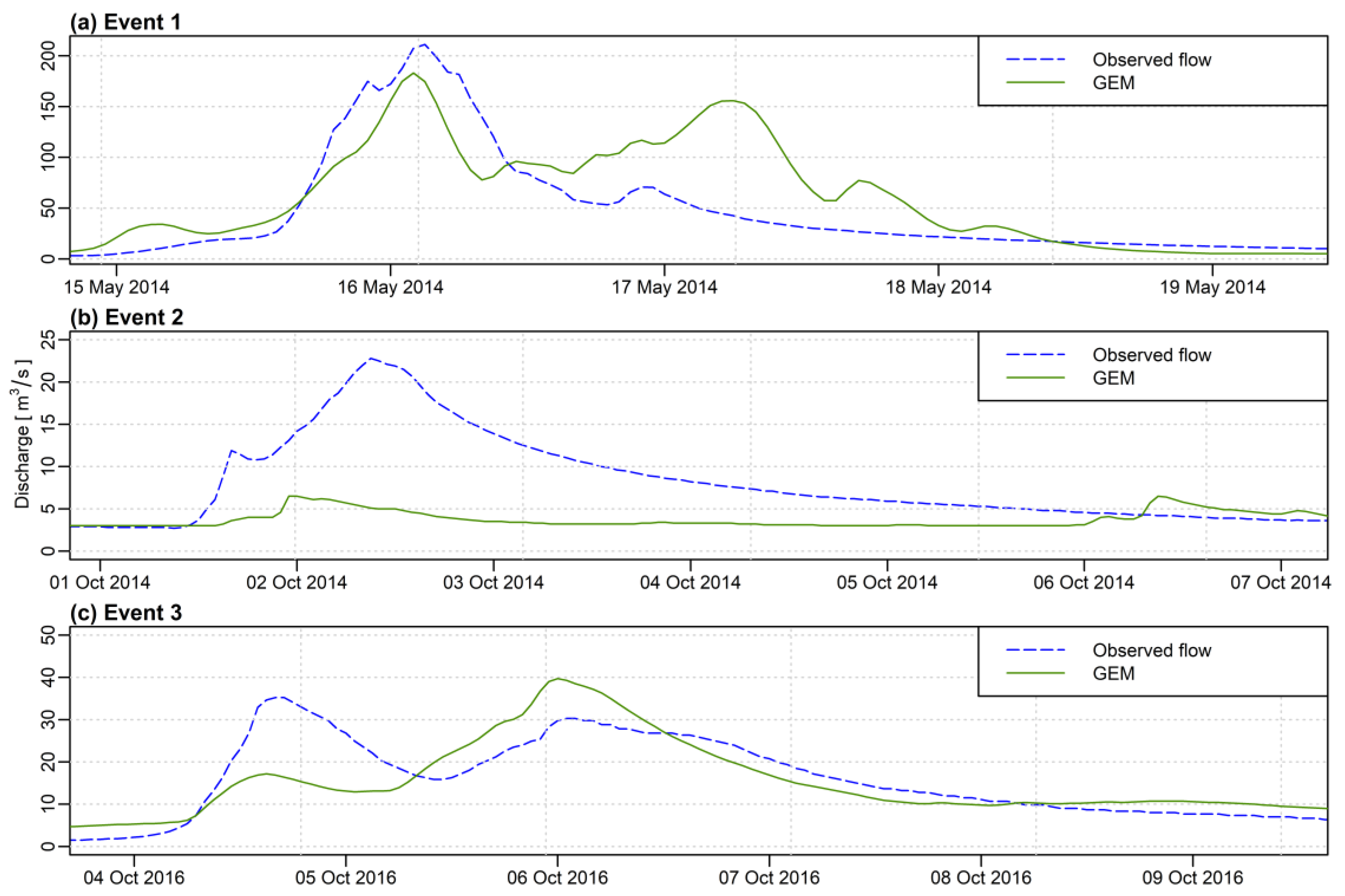
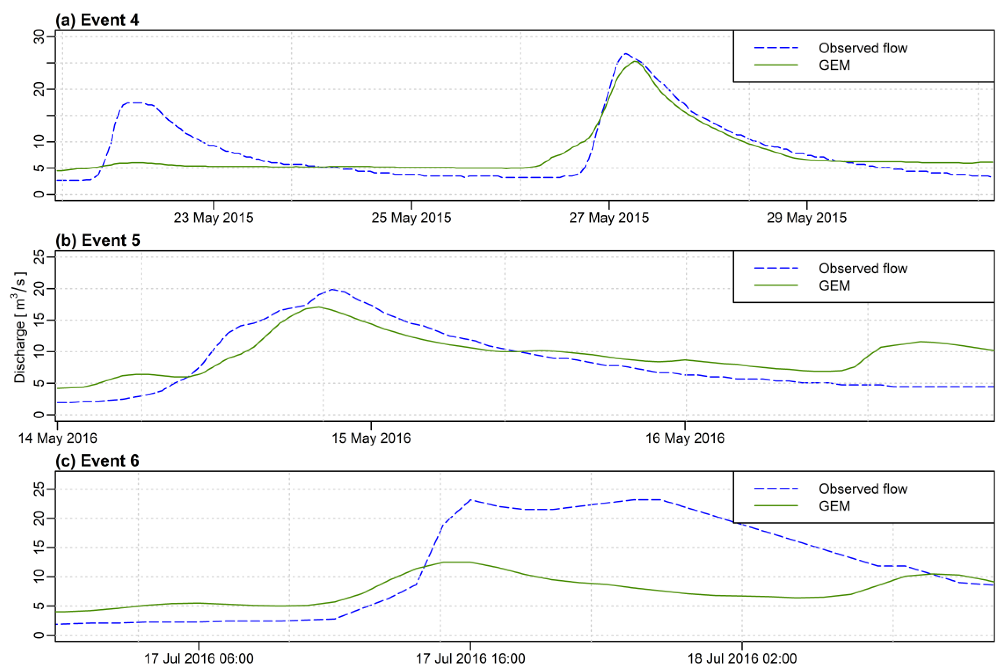
Precipitation data for rain gauge and GEM, as well as discharge data, were obtained between 2014 and 2016. During this interval, there were six flood events. Three of them were used for the calibration of the model, while the other three were used for its calibration.

Other data used in the study were the Digital Elevation Model (DEM) of 100 m resolution that was provided by the Head Office of Geodesy and Cartography in Poland and land-use data from the CORINE Land Cover Project 2018. Statistical analysis and data processing were performed using R software version 4.2.1 developed at Bell Laboratories (downloaded from the website of Imperial College London, United Kingdom).

2.3. Rainfall-Runoff Modeling and Assessment

Rainfall–runoff hydrological modeling was performed using Hydrologic Engineering Center-Hydrologic Modelling System (HEC-HMS) version 4.9. It is a freeware software developed by the US Army Corps of Engineers that enables continuous and event-based hydrological modeling. Depending on the selected parameters, the model can be used in a lumped or semi-distributed mode and is widely used for flood simulations in various scientific applications [30,31,32]. The HEC-HMS model was linked with HEC-DSSVue software version 2.0.1 developed by the US Army Corps of Engineers to provide precipitation and discharge data. Both softwares. HEC-HMS and HEC-DSSVue, were downloaded from the website of US Army Corps of Engineers.

For the purpose of this work the model was adopted in a semi-distributed scheme using the following parameters for the catchment model:

• Rainfall losses—Soil Conservation Service (SCS) Curve Number (CN);
• Transformation of effective precipitation—Snyder unit hydrograph;
• Baseflow—Recession baseflow;
• Routing—Musingum–Cunge.

As for the meteorological model, the specified hyetographs were applied for every sub-catchment for each data source of precipitation (rain gauge and GEM). During the calibration phase, the following parameters were calibrated:

• Initial abstraction and curve number (for the rainfall loss method);
• Standard lag and peaking coefficient (for the transformation of effective precipitation).

The peak-weighted RMSE metric was applied as an objective function during the calibration of the model. The simulated discharge was compared to the observed flow registered at the gauging station in Osielec. Simulations were performed at hourly time-steps.

To provide multi-aspect analysis during the calibration and validation phase, the following evaluation metrics were chosen (

Table 3. Evaluation metrics adopted in the study.

Metric	Aim	Criteria	Reference
Nash–Sutcliffe Efficiency coefficient (NSE)	To assess the predictive power of the model	Values range from −∞ to 1. NSE = 1 means that the simulated flow matches perfectly to the observed one, whereas NSE = 0 means that the accuracy of predictions from the model corresponds to the mean of the observations. In case NSE < 0, it indicates that the mean of observed flow would be a better prediction than the model	[33]
Root Mean Square Error (RMSE)	To provide information on the standard deviation of the model prediction error	The smaller the value, the better the model performance. RMSE equal to 0 means a perfect match.
Percent Bias (PBias)	To assess the model performance regarding the tendency to over- or underestimate the simulated flow	Values > 20% are considered as unacceptable	[34]
Pearson’s correlation coefficient (r)	To measure the degree of linear association between observed and simulated discharge	Values range from −1 to 1. Absolute values ≤ 0.4 are considered unsatisfactory.

).

2.4. Calculation of Antecedent Moisture Conditions

Moisture conditions for each sub-catchment were defined by assigning a so-called Antecedent Moisture Condition (AMC) group. A distinction was made between three AMC groups depending on the amount of antecedent precipitation:

• AMC I—the lowest probability of surface runoff;
• AMC II—a moderate probability of surface runoff occurrence;
• AMC III—the highest probability of surface runoff.

The methodology for assigning an AMC group for a given sub-catchment is to calculate the sum of precipitation from the 5 days preceding the flood event and then attribute an AMC group in accordance with

Table 4. AMC groups according to precipitation totals [35].

AMC Group	Total Precipitation [mm]
	Non-Growing Season	Growing Season
I	<13	<35
II	13–28	35–53
III	>28	>53

. A distinction was made between the growing season and the non-growing season, which were characterized by different precipitation thresholds.

Moisture conditions must be determined for each flood period before running the simulation. The AMC factor does not have tolerance ranges, but rigid limits that cause a change in group assignment. Therefore, it can be assumed that it does not reflect the actual dynamics of changes in effective precipitation. In order to increase the precision of the estimation of moisture conditions, it would be necessary to take into account, among other things, temperature or insolation, which can significantly affect wetness. For this reason, in order to simplify the subsequent calibration process of the CN coefficient and to minimize the spatial variability of moisture content, a common solution is to calculate the antecedent precipitation totals for sub-catchments by assigning to them the precipitation sums from the nearest meteorological station.

AMC conditions were determined for sub-catchments using two data sources of precipitation–rain-gauge data and GEM. It was decided to carry that out due to the fact that precipitation data from meteorological stations are mostly used for this purpose and will serve as a valuable reference to the AMC classification obtained from GEM data. Using the precipitation fields created by the Inverse Distance Weighting (IDW) interpolation, the area average precipitation total for each sub-catchment was calculated, and the corresponding AMC group number was assigned. It was decided to carry that out in order to account for the greater spatial variability of precipitation. The IDW method was chosen for the calculations due to the fact that it is the primary method of interpolating precipitation built into the HEC-HMS hydrological model and because of the very good flow simulation results obtained using this interpolation method [36,37]. When using data from the GEM model, a weighted average proportional to the area of the GEM pixel covering a given sub-basin was calculated. For both data sources, 5-day precipitation totals were calculated based on 1 h accumulations. All investigated flood events during the calibration and validation phases corresponded to the growing season.

3. Results

3.1. Discharge Simulations for Calibration Events

Figure 4 shows the comparison of the simulated and observed discharge for calibration events. All simulations were performed at hourly time steps. In

Table 5. The results of the evaluation criteria for calibration events.

Event	Metric
	NSE	RMSE	PBias [%]	r
Event 1	0.79	37.79	1.7	0.90
Event 2	−0.76	6.28	63.4	0.79
Event 3	0.54	6.68	−3.2	0.54

, the results of evaluation criteria are provided. To directly investigate the impact of precipitation data on the hydrological model, only parameters for SCS curve number method (rainfall losses) were calibrated.

Considering the calibration events, it can be noted that, for Event 1 and Event 3, the results are acceptable or good. What is notable about these two events is that the results from the hydrological model tend to overestimate the second peak occurring in the river. However, when it comes to the peak flow values, the difference between the simulated and observed flow is not very significant and can be used as a reliable predictive value. For Event 2, which represents the smallest flood event, the GEM model tends to provide such low precipitation values, which are insufficient in representing the flood event. It is worth noting that the best flow simulation results were obtained for flood Event 1, which is characterized by a very high maximum flow. This shows the great potential of using GEM data in simulating large floods. For that event, the RMSE value is significantly higher than for other events due to a much higher discharge.

3.1.1. AMC Conditions and Rainfall Losses Calibration

Moisture conditions in the catchment are one of the key elements during the formation of surface runoff, which can lead to flooding. Therefore, prior to the calibration of the CN method parameters, the AMC classification for every sub-catchment was made (

Table 6. AMC classification for sub-catchment according to Table 4.

Sub-Catchment	Event 1				Event 2				Event 3
	Rain Gauge		GEM		Rain Gauge		GEM		Rain Gauge		GEM
	P [mm]	AMC	P [mm]	AMC	P [mm]	AMC	P [mm]	AMC	P [mm]	AMC	P [mm]	AMC
SC-1	23.6	I	23.3	I	32.6	I	8.9	I	29.7	I	4.6	I
SC-2	21.8	I	34.8	I	16.6	I	16.2	I	29.6	I	6.0	I
SC-3	22.8	I	28.6	I	18.8	I	14.5	I	37.3	II	5.8	I
SC-4	23.1	I	44.0	II	18.4	I	15.6	I	36.6	II	6.5	I
SC-5	24.1	I	29.0	I	17.9	I	9.6	I	36.1	II	5.8	I
SC-6	30.2	I	24.4	I	15.9	I	5.7	I	36.9	II	7.6	I

).

According to the table above, we can notice that, in most of the cases, both data sources of precipitation indicate the same AMC classification for the sub-catchment. Most differences occur for Event 3, but we must keep in mind that sub-catchments 3–6 were classified as AMC II, exceeding the precipitation value for AMC I by less than 2 mm of precipitation. For the big precipitation events, such as Event 1, the GEM model tends to provide higher precipitation values than rain gauge data, whereas, for the smaller ones (events 2 and 3), the rain gauge data provide significantly higher values.

The classification of a sub-catchment into a given AMC group has direct implications for parameter estimation in the SCS-CN method. The concept of this method is based on the curve number methodology. The excess of precipitation is assessed as a function of land-use, soil cover, and moisture content prior to the flood event. For each sub-catchment on the basis of land-use and fraction of impervious areas, a weighted value of CN was estimated. Values of curve numbers were taken from standard tables [38]. In

Table 7. Estimated parameters for the SCS-CN method (CN—curve number; I_a—initial abstraction).

Sub-Catchment	AMC I		AMC II		AMC III
	CN [-]	Ia [mm]	CN [-]	Ia [mm]	CN [-]	Ia [mm]
SC-1	41.18	27.21	61.46	11.95	79.90	6.39
SC-2	43.02	25.23	64.21	10.62	83.47	7.55
SC-3	50.88	18.39	69.70	8.28	84.33	7.08
SC-4	52.82	17.01	72.36	9.70	87.56	5.41
SC-5	51.51	17.39	70.56	10.60	85.38	6.52
SC-6	51.73	17.77	70.87	10.44	85.75	6.33

, the values of the curve number parameter (CN) and initial abstraction (I_a) for all AMC groups are provided.

Given that most of the sub-catchments were classified as AMC I, the initial values of the curve number and initial losses were assumed to be those calculated for AMC I. Initially, a calibration process was carried out for these two parameters without setting an upper limit on the values. It turned out that, for four of the six catchments, the optimized parameter values corresponded with those for AMC III conditions. Based on the specified moisture conditions, we can conclude with a fairly high degree of certainty that the optimized parameter values should not exceed the AMC II group. Therefore, in the next iteration of model calibration, the upper limits of the parameter values were set as those corresponding to AMC II. The final results of the optimized parameter values are shown in

Table 8. Comparison of the initial and optimized values of parameters of the CSC-CN method.

Sub-Catchment
SC-1	SC-2	SC-3	SC-4	SC-5	SC-6
Initial Value/Optimized Value
Initial abstraction [mm]
25.23/20.09	27.21/25.02	17.77/15.37	17.39/14.83	17.01/13.88	18.39/17.46
CN value [-]
43.02/39.97	41.18/53.59	51.73/56.34	51.51/56.29	52.82/54.22	50.88/59.92

.

During calibration, the model for sub-catchments 2–6 indicates higher CN values than the initial ones. On average, these values are 10–30% higher. Only for sub-catchment SC-1 is the optimized value lower. For all sub-catchments, the optimized initial abstraction values are lower than the initial ones.

3.1.2. Discharge Simulations for Validation Events

Another three events were chosen for the validation of the model. The hydrological model was run with optimized values of curve numbers and initial abstractions for the sub-catchments. Other parameters were not changed.

Figure 5 shows the comparison of simulated and observed discharge for validation events. Simulations by the model were performed at hourly time steps. In

Table 9. The results of the evaluation criteria for validation events.

Event	Metric
	NSE	RMSE	PBias [%]	r
Event 4	0.67	6.34	−5.6	0.83
Event 5	0.58	3.21	−13.9	0.83
Event 6	0.15	0.54	−46.1	0.57

, the results of the evaluation criteria are provided.

The level of agreement between modeled and observed flow validation results are very similar to the model calibration phase. Good results have been obtained for Event 4, acceptable for Event 5, and unsatisfactory for Event 6. An interesting observation occurs in Event 4. The first peak is not mapped at all, whereas the second is simulated almost perfectly. This shows that GEM data perform worse in mapping precipitation for small values, which are then transformed through surface-runoff into small flood events.

4. Summary and Conclusions

The purpose of this paper was to present the potential of using numerical weather prediction data from a Global Environmental Multiscale model for rainfall–runoff hydrological modeling in a small mountain catchment. The analysis explored the feasibility of using GEM data to simulate discharge and determine antecedent moisture conditions in the catchment.

It is worth noting that, according to the literature review conducted by the article’s author, this is the first published attempt to use GEM data directly in applied hydrological applications, such as event-based modeling, for a small mountainous catchment. Previous works using GEM data have focused only on strictly meteorological aspects (e.g., [39,40,41]) or continuous hydrological modeling on large catchments.

Based on the analysis, the following conclusions can be drawn:

• GEM data can be used for rainfall–runoff modeling with satisfactory results. Since these data are available in advance, they can be used to conduct a preliminary forecast of discharge.
• Better results of the projected outflow were obtained for heavy rainfall events (Events 1, 3 and 4). For relatively small rainfall events, the GEM data appear to underestimate the amount of precipitation, resulting in a consequent underestimation of the simulated flow rate.
• Overall, the best simulation results were obtained for Event 1, which has the highest value of maximum flow. This may indicate a significant potential for the use of GEM data to forecast large floods.
• GEM data can be useful for determining moisture conditions in the catchment area. Assigned AMC groups for sub-catchments were very close to those determined from the rain gauge data. This is a very important advantage of these data, especially if they would allow us to determine in advance that we may be dealing with AMC Group III, where the consequences of which could be very large floods.
• Moisture conditions are often a neglected aspect during hydrological modeling, but, as shown during the calibration process, they play a vital role. The correct identification of AMC groups allows us to determine the range of values of the parameters of the rainfall losses model closer to reality. In particular, it is a matter of limiting unrealistic calibration results, which can give parameter values for a higher AMC group.
• A significant disadvantage of the SCS-CN model in determining its parameters is the rigid limits in the classification adopted (Table 4). Another aspect is the uncertainty associated with the correct determination of conditions in the catchment from the point of view of vegetation and land use, which affects the estimated parameters. Therefore, the determined values of the model parameters should be approached not deterministically but with a significant amount of tolerance at the calibration phase.
• Despite the fact that GEM data do not perform the best in forecasting small-scale flood events, they can still be successfully used to determine the AMC in such cases.

It should be noted that the presented discharge simulation results were unsatisfactory in several cases. Given that only parameters related to precipitation losses were calibrated in the hydrological model, it seems that the main reason for such results is the inaccuracy of the GEM data. In particular, this is an underestimation of rainfall for small events, which leads to better-projected discharge for heavy rainfall events and worse for small rainfall events. Due to dynamic processes in the atmosphere, forecasting precipitation is complex, and, as shown in Table 6, there are often underestimations for small events. For significant rainfall events, forecast values can often be higher than those that occur in reality. On the other hand, if the hydrological model is properly calibrated, this does not necessarily lead to an overestimation of the predicted discharge.

In order to accurately analyze the sources of errors that lead to the obtained results, it is necessary to consider the errors directly related to the GEM data separately, as well as the errors resulting from the specifics of the hydrological model. For example, it would be interesting to validate the GEM data using the rain gauge data or to adjust the bias using high-resolution satellite data. As for the hydrological model, the current version used for validation could be recalibrated using other model parameters that were not calibrated. In such an approach, however, it should be kept in mind that there could be a situation of model over-calibration, which could lead to unrealistic results.

In future work, it would be interesting to compare the determination of AMC conditions for the catchment area using other precipitation data, such as satellites and meteorological radars. It would also be necessary to verify what the effect of the interpolation method for rain gauge data on AMC classification is. Another interesting aspect from a hydrological point of view is a separate analysis of errors from GEM’s outputs and the HEC-HMS hydrological model.

References

1. Stocker, T. (Ed.) Climate Change 2013: The Physical Science Basis: Working Group I Contribution to the Fifth Assessment Report of the Intergovernmental Panel on Climate Change; Cambridge University Press: Cambridge, UK, 2014. [Google Scholar]
2. Fabry, F.; Bellon, A.; Duncan, M.R.; Austin, G.L. High resolution rainfall measurements by radar for very small basins: The sampling problem reexamined. J. Hydrol. 1994, 161, 415–428. [Google Scholar] [CrossRef]
3. Beven, K.J. Rainfall-Runoff Modelling: The Primer; John Wiley & Sons: Hoboken, NJ, USA, 2012; ISBN 9781119951001. [Google Scholar]
4. Abbe, C. The physical basis of long-range weather forecasts. Mon. Weather Rev. 1901, 29, 551–561. [Google Scholar] [CrossRef]
5. Bjerkenes, V. Das Problem der Wettervorhersage, betrachtet vom Standpunkt der Physik und Mechanik. Meteorol. Z. 1904, 21, 1–7. [Google Scholar]
6. Bauer, P.; Thorpe, A.; Brunet, G. The quiet revolution of numerical weather prediction. Nature 2015, 525, 47–55. [Google Scholar] [CrossRef] [PubMed]
7. Jasper, K.; Gurtz, J.; Lang, H. Advanced flood forecasting in Alpine watersheds by coupling meteorological observations and forecasts with a distributed hydrological model. J. Hydrol. 2002, 267, 40–52. [Google Scholar] [CrossRef]
8. Yucel, I.; Onen, A.; Yilmaz, K.K.; Gochis, D.J. Calibration and evaluation of a flood forecasting system: Utility of numerical weather prediction model, data assimilation and satellite-based rainfall. J. Hydrol. 2015, 523, 49–66. [Google Scholar] [CrossRef]
9. Mahdi, E.; Khalki, E.; Tramblay, Y.; El, M.; Saidi, M.; Bouvier, C.; Hanich, L. Comparison of modeling approaches for flood forecasting in the High Atlas Mountains of Morocco. Arab. J. Geosci. 2018, 11, 1–15. [Google Scholar]
10. Bartholmes, J.; Todini, E. Coupling meteorological and hydrological models for flood forecasting. Hydrol. Earth Syst. Sci. Discuss. 2005, 9, 333–346. [Google Scholar] [CrossRef]
11. Barnier, B.; Siefridt, L.; Marchesiello, P. Thermal forcing for a global ocean circulation model using a three-year climatology of ECMWF analyses. J. Mar. Syst. 1995, 6, 363–380. [Google Scholar] [CrossRef]
12. Takenaka, H.; Nakajima, T.Y.; Higurashi, A.; Higuchi, A.; Takamura, T.; Pinker, R.T.; Nakajima, T. Estimation of solar radiation using a neural network based on radiative transfer. J. Geophys. Res. Atmos. 2011, 116, 1–26. [Google Scholar] [CrossRef]
13. Gaborit, É.; Fortin, V.; Xu, X.; Seglenieks, F.; Tolson, B.; Fry, L.M.; Hunter, T.; Anctil, F.; Gronewold, A.D. A hydrological prediction system based on the SVS land-surface scheme: Efficient calibration of GEM-Hydro for streamflow simulation over the Lake Ontario basin. Hydrol. Earth Syst. Sci. 2017, 21, 4825–4839. [Google Scholar] [CrossRef]
14. Rokaya, P.; Morales-marin, L.; Lindenschmidt, K. Towards Improved Real-time Forecasting of River Ice Breakup. In Proceedings of the 20th Workshop on the Hydraulics of Ice Covered Rivers, Ottawa, ON, Canada, 14–16 May 2019. [Google Scholar]
15. Abaza, M.; Fortin, V.; Gaborit, É.; Bélair, S.; Garnaud, C. Assessing 32-Day Hydrological Ensemble Forecasts in the Lake Champlain–Richelieu River Watershed. J. Hydrol. Eng. 2020, 25, 1–13. [Google Scholar] [CrossRef]
16. Asong, Z.E.; Elshamy, M.E.; Princz, D.; Wheater, H.S.; Pomeroy, J.W.; Pietroniro, A.; Cannon, A. High-resolution meteorological forcing data for hydrological modelling and climate change impact analysis in the Mackenzie River Basin. Earth Syst. Sci. Data 2020, 12, 629–645. [Google Scholar] [CrossRef]
17. Côté, J.; Gravel, S.; Mé, A.; And, T.; Patoine, A.; Roch, M.; Staniforth, A. The Operational CMC-MRB Global Environmental Multiscale (GEM) Model. Part I: Design Considerations and Formulation. Mon. Weather Rev. 1998, 126, 1373–1395. [Google Scholar] [CrossRef]
18. Kamiński, J.W.; Neary, L.; Strużewska, J.; Mcconnell, J.C.; Lupu, A.; Jarosz, J.; Toyota, K.; Gong, S.L.; Côté, J.; Liu, X.; et al. GEM-AQ, an on-line global multiscale chemical weather modelling system: Model description and evaluation of gas phase chemistry processes. Atmos. Chem. Phys. 2008, 8, 3255–3281. [Google Scholar] [CrossRef]
19. Strużewska-Krajewska, J.; Kamiński, J.; Durka, P.; Jefimow, M. Sprawdzalność Operacyjnej Prognozy Stanu Jakości Powietrza Dla Obszaru Województwa Małopolskiego W Okresie Od Grudnia 2013 Do Września 2014; Report no 501H/1110/5734; Warszawa, Poland, 2014. (In Polish) [Google Scholar]
20. Deardorff, J.W. Efficient prediction of ground surface temperature and moisture, with inclusion of a layer of vegetation. J. Geophys. Res. 1978, 83, 1889. [Google Scholar] [CrossRef]
21. Bougeault, P.; Lacarrere, P. Parameterization of orography-induced turbulence in a mesobeta-scale model. Mon. Weather Rev. 1989, 117, 1872–1890. [Google Scholar] [CrossRef]
22. Bélair, S.; Mailhot, J.; Girard, C.; Vaillancourt, P. Boundary layer and shallow cumulus clouds in a medium-range forecast of a large-scale weather system. Mon. Weather Rev. 2005, 133, 1938–1960. [Google Scholar] [CrossRef]
23. Sundqvist, H. A parameterization scheme for non-convective condensation including prediction of cloud water content. Q. J. R. Meteorol. Soc. 1978, 104, 677–690. [Google Scholar] [CrossRef]
24. Kain, J.S.; Fritsch, J.M. A one-dimensional entraining/detraining plume model and its application in convective parameterization. J. Atmos. Sci. 1990, 47, 2784–2802. [Google Scholar] [CrossRef]
25. Fouquart, Y.; Bonnel, B. Computations of solar heating of the earth’s atmosphere: A new parameterization. Contrib. Atmos. Phys. 1980, 53, 35–62. [Google Scholar]
26. Garand, L. Some improvements and complements to the infrared emissivity algorithm including a parameterization of the absorption in the continuum region. J. Atmos. Sci. 1983, 40, 230–244. [Google Scholar] [CrossRef]
27. McFarlane, N.A. Interactions between orographic gravity wave drag and forced stationary planetary waves in the winter northern hemisphere middle atmosphere. J. Atmos. Sci. 1987, 44, 1775–1800. [Google Scholar] [CrossRef]
28. McLandress, C.; McFarlane, N.A. Interactions between orographic gravity wave drag and forced stationary planetary waves in the winter northern hemisphere middle atmosphere. J. Atmos. Sci. 1993, 50, 1966–1990. [Google Scholar] [CrossRef]
29. Szturc, J.; Jurczyk, A.; Ośródka, K.; Wyszogrodzki, A.; Giszterowicz, M. Precipitation estimation and nowcasting at IMGW-PIB (SEiNO system). Meteorol. Hydrol. Water Manag. 2018, 6, 3–12. [Google Scholar] [CrossRef]
30. Knebl, M.R.; Yang, Z.L.; Hutchison, K.; Maidment, D.R. Regional scale flood modeling using NEXRAD rainfall, GIS, and HEC-HMS/ RAS: A case study for the San Antonio River Basin Summer 2002 storm event. J. Environ. Manag. 2005, 75, 325–336. [Google Scholar] [CrossRef]
31. Halwatura, D.; Najim, M.M.M. Application of the HEC-HMS model for runoff simulation in a tropical catchment. Environ. Model. Softw. 2013, 46, 155–162. [Google Scholar] [CrossRef]
32. Rauf, A.U.; Ghumman, A.R. Impact assessment of rainfall-runoffsimulations on the flow duration curve of the Upper Indus river-a comparison of data-driven and hydrologic models. Water (Switzerland) 2018, 10, 876. [Google Scholar] [CrossRef]
33. Nash, J.E.; Sutcliffe, J.V. River flow forecasting through conceptual models part I—A discussion of principles. J. Hydrol. 1970, 10, 282–290. [Google Scholar] [CrossRef]
34. Fang, G.; Yuan, Y.; Gao, Y.; Huang, X.; Guo, Y. Assessing the Effects of Urbanization on Flood Events with Urban Agglomeration Polders Type of Flood Control Pattern Using the HEC-HMS Model in the Qinhuai River Basin, China. Water 2018, 10, 1003. [Google Scholar] [CrossRef]
35. Soczyńska, U. Hydrologia Dynamiczna; Wydawnictwo Naukowe PWN: Warszawa, Poland, 1997. [Google Scholar]
36. Garcia, M.; Peters-Lidard, C.D.; Goodrich, D.C. Spatial interpolation of precipitation in a dense gauge network for monsoon storm events in the southwestern United States. Water Resour. Res. 2008, 44, 1–14. [Google Scholar] [CrossRef]
37. Cheng, M.; Wang, Y.; Engel, B.; Zhang, W.; Peng, H.; Chen, X.; Xia, H.; Cheng, M.; Wang, Y.; Engel, B.; et al. Performance Assessment of Spatial Interpolation of Precipitation for Hydrological Process Simulation in the Three Gorges Basin. Water 2017, 9, 838. [Google Scholar] [CrossRef]
38. Kibler, D.F. Urban Stormwater Hydrology; American Geophysical Union: Washington, DC, USA, 1982. [Google Scholar]
39. Lin, C.; Vasić, S.; Kilambi, A.; Turner, B.; Zawadzki, I. Precipitation forecast skill of numerical weather prediction models and radar nowcasts. Geophys. Res. Lett. 2005, 32, 1–4. [Google Scholar] [CrossRef] [Green Version]
40. Surcel, M.; Berenguer, M.; Zawadzki, I. The diurnal cycle of precipitation from continental radar mosaics and numerical weather prediction models. Part I: Methodology and seasonal comparison. Mon. Weather Rev. 2010, 138, 3084–3106. [Google Scholar] [CrossRef]
41. Zdunek, M.; Kłęczek, M. Performance of GEM-LAM dichotomous forecast for selected weather phenomena. Sci. Rev. Eng. Environ. Sci. 2016, 25, 483–496. [Google Scholar]
Figure 1. Main characteristics of the study area (elevation, and locations of meteo stations and gauging stations. Sub-catchments)—upper part of the Skawa catchment.
Atmosphere 13 01348 g001
Figure 2. GEM computational grid: global model (left) with variable resolution (0.135° over Europe) and nested grid over Poland (right) with a resolution of 0.0625° [19].
Atmosphere 13 01348 g002
Figure 3. One-hour rainfall accumulations from the GEM forecasting model over the upper Skawa catchment.
Atmosphere 13 01348 g003
Figure 4. Simulated and observed discharge for calibration events (a) Event 1: 14–23 May 2014, (b) Event 2: 3–7 October 2014, (c) Event 3: 3–9 October 2016.
Atmosphere 13 01348 g004
Figure 5. Simulated and observed discharge for validation events (a) Event 4: 21–30 May 2015, (b) Event 5: 14–17 May 2016, (c) Event 6: 17–19 July 2016.
Atmosphere 13 01348 g005