Modeling the Interdependence Structure between Rain and Radar Variables Using Copulas: Applications to Heavy Rainfall Estimation by Weather Radar

Abstract

In radar quantitative precipitation estimates (QPE), the progressive evolution of rainfall algorithms has been guided by attempts to reduce the uncertainties in rainfall retrieval. However, because most of the algorithms are based on the linear dependence between radar and rain variables and designed for rain rates ranging from light to moderate rainfall, they result in misleading estimations of intense or strong rainfall rates. In this paper, based on extensive data gathered during the AMMA and Megha-Tropiques data campaigns, we provided a way to improve the estimation of intense rainfall rates from radar measurements. To this end, we designed a formulation of the QPE algorithm that accounts for the co-dependency between radar observables and rainfall rate using copula simulation synthetic datasets and using the quantile regression features for a more complete picture of covariate effects. The results show a clear improvement in heavy rainfall retrieval from radar data using copula-based R(K_DP) algorithms derived from a realistic simulated dataset. For a better performance, Gaussian copula-derived algorithms require a 0.8 percentile distribution to be considered. Conversely, lower percentiles are better for Student’s, Gumbel and HRT copula estimators when retrieving heavy rainfall rates (R > 30). This highlights the need to investigate the entire conditional distribution to determine the performance of radar rainfall estimators.

1. Introduction

Measurement by remote sensing stands as a unique tool for continuous coverage in time and space. For instance, a weather radar provides real-time spatially continuous measurements covering a large area within short time intervals. This is important for better catching spatial rainfall variability and is useful when modeling the hydrological behavior of watersheds. Because radar rainfall measurements are not direct, conventional modes of radar rainfall estimation use a parametric relation ($Z-R$). This relationship is often formulated based on measurements of radar reflectivity and ground rain gauge rainfall or from raindrop size distributions (DSD). However, the conversion of $Z$ in $R$ presents numerous errors, including the variability of a reflectivity vertical profile [1], the error in measuring radar reflectivity [2,3], the variability of rainfall drop size distribution [4,5,6,7,8,9,10], the nature of rainfall [11,12,13,14], the data analysis method [15] and the use of point rainfall measurements on the ground as corresponding to radar pixel-averaged values [16,17,18] (mismatch of sampling volume between radar and rain gauge observations). Because the major source of error in the $Z-R$ precipitation algorithm is the variability in the drop size distribution, error reduction attempts in radar rainfall estimation have been suggested by several authors with a distinction between the convective or stratiform nature of DSD-based algorithms. However, the results were disappointing as they barely differed from those obtained by using a unique relationship $Z-R$ [13,19]. Steiner et al. [4], using simulations, and Ochou et al. [9] and Bamba et al. [10], based on DSD observations in West Africa, emphasized that understanding the variability of the $Z-R$ relation includes taking into account the simultaneous variability of the size and number of raindrops. Although the implementation of such approaches is difficult in an operational way, these studies suggest, because of numerous combinations of size and the number of drops, that additional radar parameters are necessary to better characterize the rain media by describing the microstructure of clouds.

The most used approaches to overcome the problem of $Z-R$ dependence on the characteristics of the drop size distributions are related to the polarimetric radar technique, and dual polarization capability is a standard for weather radars today. Indeed, based on the anisotropy of the rain medium induced by the oblateness of raindrops, new polarimetric radar variables such as the differential reflectivity Z_DR and the specific differential phase shift K_DP are provided to design rainfall estimators that are less sensitive to variations in precipitation parameters. Since Z_DR is related to drop size median volume diameter D₀ [20,21], a combined two-parameter algorithm [R(Z_H, Z_DR)] was used to estimate rainfall [22,23] and was found to be less dependent on the DSD variability than $Z-R$. Many other authors proposed the combination of K_DP and Z_DR [24,25,26], which means that the effect of DSD variability on both variables compensate for one other [8], or the construction of a three-parameter algorithm [27,28], which implicitly accounts for variability in drop shape (thus in drop size). Combined rain estimators have an important advantage in that each of the included radar polarimetric variables provide different information either on the distribution of raindrops or the type of hydrometeors, or the shape of the drops. However, enhancing the number of radar variables in algorithms increases the risk of uncertainties because of noisy measurements due to fluctuations in the differential phase or differential reflectivity, especially in the cases of light rain and the attenuation correction problem (for X-band radar) affecting reflectivity without having the certainty of improving the rainfall estimation results. Recently, Koffi et al. [29], comparing four polarimetric algorithms, found that the simple polarimetric one-parameter estimator R(K_DP) outperformed all other combined estimators for the highest rain rates (above 30 mm/h), probably because of the quasi-linear nature of the relationship, which makes it less sensitive to fluctuations in DSD. However, work from [8] revealed its sensitivity to range intensity and to event-to-event variability, even though this fact was more pronounced for multi-parameter algorithms. Efforts are needed to optimize the algorithms by addressing some remaining important issues.

Several possible reasons exist to explain the variable performance and related significant uncertainties of rainfall estimators. One reflects the difficulty in modeling the dependence between radar variables and radar-rain variable relationships in a Gaussian framework generally used for this purpose. Indeed, the dependence parameter used for assessing these relations is the linear Pearson correlation. This linear correlation indicator is efficient when the dependency relationship is linear and the universe is considered Gaussian. The linear correlation coefficient, which is the most used measure to test dependence between variables, is only a measure of linear dependence. This means that it is a meaningful measure of dependence if variables are well represented by elliptical distribution. Outside the world of elliptical distributions, however, using the linear correlation coefficient as a measure of dependence may lead to misleading conclusions. For example, when it comes to integrating the whole rain rate range or only extreme values in an algorithm’s calibration, the assumption of linear dependence is not reliable. Furthermore, when choosing the full rain rate range, the linear-dependent structure could not be adequately captured in a Gaussian framework. Hence, alternative methods for capturing co-dependency should be considered; unfortunately, this setting is rarely included when modelling the link between the extreme values of two or more variables.

The second plausible reason for the inadequate performance of rainfall algorithms is the limitation of datasets used to derive statistical radar rainfall estimators. Regression-based relationships often derive from (i) an analysis of datasets of limited observed drop size distributions (DSD) [8,27,29,30], (ii) unrealistic simulated DSD [22,23,31,32] for the numerical simulation of useful radar variables or (iii) a comparison of radar data and rain gauges rain rates [29], both with a different sampling volume. Such estimators are thus determined to have significant uncertainties due to limited datasets (I, iii), an unrealistic nature (ii), difference in sampling between radar and rain gauge (iii) and fluctuation with data variation (i, iii). Therefore, algorithms that are determined based on such limited databases do not perform well in most cases where they are applied. For instance, in most algorithm calibrating data samples, weak to moderate rain rates are significant, numerous and govern the algorithms’ coefficients. This could reduce the performance of the related algorithms to retrieve the highest rain rates that can contribute significantly to the total accumulated rainfall.

Finally, the regression method used to determine estimators is based on logarithm transformation of variables with the risk of changing the nature of addiction between them since the Pearson linear correlation coefficient is dependent on the monotonic function applied to the variables. For all these reasons, it appears that another setup for realistic synthetic datasets based on advanced statistical models could be useful. The aim of this statistical approach is to increase the weighting of the high (or extreme) values in the fitting processing steps and thus to assess how successful the method is in improving quantitative precipitation estimates.

In this context, to overcome the above-mentioned limits, the approach of the copula theory is an innovative tool for both modeling the dependence structure between several random variables without necessarily making the assumption of a Gaussian framework or a linear dependence between them and generating realistic synthetic data, including a sufficient sample of extreme values useful for determining rainfall estimators based on the incorporation of a broad range of variables of interest. Copula tools have long drawn interest in quantitative financial applications, e.g., in the measurement of multiple credit or market risks [33,34], the replication of hedge fund performance and actuarial science [35] and portfolio management using Monte Carlo simulations. Given the promising results of copula functions to investigate multivariate issues, in the past 10 years, there have been fast-growing applications in hydrology for flood frequency analyses [36,37,38], multivariate hydrological event frequency analyses [39,40] and hydrologic and hydraulic studies for dam breach analyses or for the adequacy of dam spillways [41,42]. In meteorology and related domains, the use of copula is relatively new and has been applied to dependence studies between drought duration and severity [43,44], drought frequency analysis [45], dependence structure between storm characteristics [46], the temporal structure of storms [47] and in introductive work from Scholzel and Friederichs [48] using the copula approach to model dependence between bivariate random variables such as daily precipitation and temperature.

In the area of radar quantitative precipitation estimation, studies based on the copula approach are few. Maity et al. [49] investigated a nonparametric approach by using a copula-based method to develop three models for the probabilistic estimation of rainfall. Therefore, the aim of this paper is twofold. First, we used copulas to model the dependence between radar and rainfall variables (specifically K_DP and R) useful to design optimal rain estimators. To this end, we used other addictive indicators based on discrepancies and concordances between the two variables of interest derived from an ‘observed’ sample in a framework not necessarily Gaussian-based and described by Pearson’s correlation coefficient. An essential practical interest in the use of copula is the ability to model the dependence between extreme values of the variables not always accounted for in radar rain estimation. We also implemented efficient algorithms for simulating bivariate joint distribution in a realistic way. Thus, the copula method allows for the generation of a synthetic dataset for differential specific phase shifts and rainfall rates, including extreme values which lack the estimator’s calibrating data that could affect its performance. From such a resulting dataset, a proper statistical method should be applied to determine optimized R(K_DP) rainfall algorithms. So far, most of the studies on the issue have determined algorithms based on conventional least squares mean regression methods. However, it has been recognized that the resulting estimates for a higher rain rate are not satisfactory, probably because the estimators could not adequately catch the effect of the upper tail of data. A more complete picture of covariate effects should be designed. We accomplished this in this research with the use of the quantile regression features to analyze performances of the R(K_DP) rainfall estimator based on simulated copula data.

In this scope, we exploited one advantage in using copulas, that is, its flexibility in choosing arbitrary marginals (the same family is not needed for each marginal distribution of variables as needed in multivariate normal distributions). The next section (Section 2) briefly reviews the concept of copula used to model the dependence structure between R and K_DP. Section 3 describes the data and the methodology employed in the study. The concepts of quantile regression and copula quantile regression are also presented, and we define formally associated rainfall retrieval algorithms. Section 4 evaluates several rain estimation models by conducting a comparison with rain gauge data used to validate the methods. Specific observed cases based on areal X-band radar data gathered during the AMMA program in Northern Benin (2006–2007) [29] and the Megha-Tropiques experiments in Niamey (Niger, West Africa) (2010) are also shown as validations of the quantile regression method by examining if better estimations of rain rates are possible. The final section (Section 5) presents a discussion of the results and offers some conclusions and perspectives.

2. Methodological Background: Basics of Copulas Theory

As this work is based on the copula approach, which is not commonly used in the radar meteorology field, an effort to resume all the related theory is made in this section. To this end, some general copula theory is provided, but many facts and definitions in the bivariate case are emphasized for the sake of simplicity.

2.1. Definitions and Properties

A copula is a distribution function of uniform marginal distribution. Specifically, a copula couples the distribution function of multivariate probability distribution to the marginal distribution functions of their coordinates [39]. Thus, if we focus our attention on the bivariate case for the sake of simplicity, copula may be written in the following form

$$\begin{array}{c}C: {\left[0;1\right]}^2\to \left[0;1\right]\\ \left(u_1,u_2\right)\to P_r\left(U_1\le u_1 , U_2\le u_2\right)\end{array}$$

(1)

where $U_1$ and $U_2$ are uniformly distributed dependent random variables for the unit interval from 0 to 1. In other words, a copula is defined as the joint cumulative distribution function (CDF) of both these uniform random variables. To provide a comprehensive definition and thus understand the importance of copula, Sklar’s theorem [50] provides a link between a multivariate distribution, its marginal distribution and a copula by establishing the inverse of the first definition. Still assuming a pair of random variables $\left(X_1, X_2\right)$ of dimension $n$ with the jointed cumulated distribution functions $F$ and marginal continuous distribution functions $F_2$, then there is an unique copula $C$, represented as follows:

$$F\left(x_1,x_2\right)=C\left(F_1\left(x_1\right), F_2\left(x_2\right)\right)=F\left(F_1^{-1}\left(u_1\right),F_2^{-1}\left(u_2\right)\right)$$

(2)

where $x_1$ and $x_2$ stand for the values where variables $X_1$ and $X_2$ are evaluated, respectively, and $F_1^{-1}\left(u_1\right)$ and $F_2^{-1}\left(u_2\right)$ are the percentiles of two distribution functions $F_1\left(x_1\right)$ and $F_2\left(x_2\right)$. This result is important in practice for applications since it indicates that an analysis of a multivariate problem can be realized in two independent stages: the identification of marginal distributions and analysis of the dependence structure between components. In other words, this representation shows the manner in which the copula function associates the joint distribution law to univariate marginal distributions. This is a prime asset for statistical investigations, since copulas allow for a wider selection of joint distribution functions regardless of the different marginal distributions considered. Furthermore, copulas can summarize the dependence of the internal structure of a random vector. The most conventional measures of dependence, such as Kendall and Spearman’s correlation, which represent the rank correlation between two random vectors, $X_1$ and $X_2$, can be expressed explicitly as a functions of the copula. With this flexibility, copula theory has applications in many fields. For details, we refer the reader to the works of Frees and Valdez [35] applied to actuarial science and finance, or those of Poulin et al. [37], Genest and Favre [51] and Favre et al. [39] for applications in hydrology. We want to extend this copula approach to the establishment of radar rainfall estimation algorithms based so far on linear correlations between radar and rain variables.

2.2. Measure of Dependence

A dependence measure regularly used for the determination of radar rainfall estimators is Pearson’s linear correlation. It measures the linear relationship between two random variables, X and Y, and can take any value in the interval from −1 to 1. This indicator is effective if the dependency relationship is linear and the universe is considered Gaussian. It is helpful for families of elliptical distributions (since for these families, non-correlation indicates independence). This dependence measure, however, has several limitations, which are as follows: (i) the correlation coefficient is not defined if the moments of order two variables are not finite; (ii) it is not an appropriate measure of dependence for heavy tail distributions where the variances can be infinite; (iii) the Pearson coefficient between two variables is not invariant to strictly increasing transformations such as logarithm functions generally used to estimate the coefficients of radar rainfall estimators (data transformations could affect the correlation and thus provide an erroneous indication of the direct relationship between these variables); and (iv) the correlation is only a scalar measure of addiction and cannot tell us everything we want to know about the structure. For extreme rainfall, we note that the Gaussian universe of radar and rain variables is not obvious, and we need to use other dependency indicators based on the similarities and discrepancies observed in a sample.

To overcome the limitations of Pearson’s linear coefficient, one can use rank-based correlation coefficients, such as Kendall’s tau and Spearman’s rho. Genest and Favre [51] explained that statistics associated with dependency structure issues between variables should be based on the ranks associated with a sample of concerned variables. These rank-based parameters are found to exhibit the invariance property (i.e., they are not affected by nonlinear changes in scale or monotonic transformations of original data) as is the case for copula [39,51], so that Schweizer and Wolff [52] suggested the expression of solely these correlation measures in terms of the copula function.

For this purpose, it may be necessary to define the concepts of concordance and discordance. Let $\left(x_1,x_2\right)$ and $\left(x_1^{*},x_2^{*}\right)$ be two realizations of continuous random two-dimensional vector $\left(X_1,X_2\right)$. $\left(x_1,x_2\right)$ and $\left(x_1^{*},x_2^{*}\right)$ are considered concordant if $\left(x_1-x_1^{*}\right)\left(x_2-x_2^{*}\right)>0$ and considered discordant if $\left(x_1-x_1^{*}\right)\left(x_2-x_2^{*}\right)<0$. Based on this definition and considering a random vector $\left(X_1,X_2\right)$, with $X_1$ and $X_2$ having a jointly continuous distribution function and $\left(X_1^{*},X_2^{*}\right)$ an independent copy of $\left(X_1,X_2\right)$, Kendall’s correlation coefficient is defined as the difference between the probability of concordance and discordance probability [35,39,52]:

$$\begin{array}{c}\tau =Pr\left\{\left(X_1-X_1^{*}\right)\left(X_2-X_2^{*}\right)>0\right\}-Pr\left\{\left(X_1-X_1^{*}\right)\left(X_2-X_2^{*}\right)<0\right\}\\ = 2 Pr\left\{\left(X_1-X_1^{*}\right)\left(X_2-X_2^{*}\right)\right\}-1\\ = 4\int CdC-1\end{array}$$

(3)

Spearman’s correlation coefficient is defined by [35,39,51]:

$$\begin{array}{c}{\rho }_S=3\left[Pr\left\{\left(X_1-X_1^{*}\right)\left(X_2-X_2^{*}\right)>0\right\}-Pr\left\{\left(X_1-X_1^{*}\right)\left(X_2-X_2^{*}\right)<0\right\}\right]\\ = 12\iint uvdC\left(u,v\right)-3\\ = 12\iint C\left(u,v\right)dvdu-3\end{array}$$

(4)

where $C$ is a copula function joining $X_1$ and $X_2$.

In practice, Kendall’s tau and Spearman’s rho reflecting the dependence between variables are empirically determined from Equations (5) and (6), which are only functions of the observations ranks of size $n$ [51].

$${\tau }_{emp}=\frac{P_n-Q_n}{\left(\begin{array}{c}n\\ 2\end{array}\right)}=\frac{4}{n\left(n-1\right)}{P}_n-1$$

(5)

$${\rho }_{emp}=\frac{12}{n\left(n+1\right)\left(n-1\right)}{\displaystyle \sum }_{i=1}^n{R}_i{S}_i-3\frac{n+1}{n-1}$$

(6)

In these relations, $\left(R_i,S_i\right)$ denotes pairs of ranks associated with the sample of the $\left(X_1,X_2\right)$ vector, and $P_n$ and $Q_n$ are numbers of concordant and discordant $\left(X_1\left[i\right],X_2\left[i\right]\right)$pairs, respectively. These dependence coefficients are also used to determine an estimate of the parameters of some selected copula through nonparametric methods [51]. For those copulas, their determination can assess the choice of the copula whose parameter has been obtained by other estimation methods discussed in the next section. For information about copulas, the reader is referred to Nelsen [53] or Genest and Favre [51].

2.3. Types and Criteria Choice of Copula

Measuring the dependence from statistical indicators such as Kendall’s tau and Spearman’s rho is different from determining the model dependence function. Copulas pursue the latter objective; as we mentioned above, these dependency indicators can be defined in this framework from the parameters of the parametric copula. In the literature, there are several families of copulas, but for this study, only a few were used. The well-known elliptical copula associated with elliptical multivariate distributions are Gaussian and Student’s copulas widely described in the work of Fang et al. [54]. These elliptical copulas are useful in practical applications due to their simplicity. Furthermore, Gaussian and Student’s copulas are derived from the multivariate normal distribution. More specifically, the Student’s copula is characterized by non-null tail-dependent coefficients, so it is suitable to connect extreme radar variables to extreme rainfall parameters. The copula expressions for both are based on $\rho$, the symmetric, positive definite correlation matrix with $diag\rho =1$, and the standardized multivariate normal ${\varphi }_{\rho }$ (for normal copula) distribution and the standardized multivariate Student’s $T_{\rho ,\upsilon }$ (for Student’s copula) distribution with $\upsilon$ degrees of freedom [39]. For a bivariate case, these elliptical copulas are defined as follows:

$$C\left(u_1,u_2,\rho \right)={\varphi }_{\rho }\left({\varphi }^{-1}\left(u_1\right),{\varphi }^{-1}\left(u_2\right)\right)$$

(7)

$$C\left(u_1,u_2,\rho ,\upsilon \right)=T_{\rho ,\upsilon }\left(t_{\upsilon }^{-1}\left(u_1\right),t_{\upsilon }^{-1}\left(u_2\right)\right)$$

(8)

where ${\varphi }^{-1}$ is the inverse univariate cumulative normal distribution and $t_{\upsilon }^{-1}$ is the inverse of the univariate Student’s distribution.

Archimedean copulas are primarily associated with the works of Genest and MacKay [55], Genest and Rivest [56] and Genest et al. [57]. The Archimedean representation reduces the study of a multivariate copula to a single univariate function. The Archimedean copulas are generated by a function $\phi$ called the generator of the copula with continuous function properties, strictly decreasing in intervals $\left(0, 1\right)$ to $\left(0, \infty \right)$, such as $\phi \left(1\right)=0$ and convex. For simplicity, we considered the bivariate copula to involute the form of the Archimedean copula proposed by Genest and Mackay (1986) for $u, v\in \left(0, 1\right)$:

$$C_{\phi }\left(u,v\right)={\phi }^{-1}\left(\phi \left(u\right)+\phi \left(v\right)\right)$$

(9)

Archimedean copulas present several desired properties, namely, symmetry, associativity and being easy to build based on the knowledge of the generating function. Moreover, for this copula type, the determination of measures of dependence is simplified. From Equation (3), Kendall’s tau is calculated as follows:

$$\tau =1+4{{\displaystyle \int }}_0^1\frac{\phi \left(u\right)}{{\phi }^{\prime }\left(u\right)}du$$

(10)

In this study, we considered the following three different bivariate Archimedean copulas expressed according to the choice of generator function: Clayton, Frank and Gumbel.

Table 1. Details (definition and parameter domain) of the copulas used in this paper.

Copula	$\mathbf{Expression}{\mathit{C}}_{\mathit{\theta }}\left(\mathit{u},\mathit{v}\right)$	Range of Dependence Parameter
Clayton	${\left(u^{-\theta }+v^{-\theta }-1\right)}^{-1/\theta }$	$\left]0, \infty \right[$
Franck	$-\frac{1}{\theta }\ln \left[1+\frac{\left(e^{-\theta u}-1\right)\left(e^{-\theta v}-1\right)}{e^{-\theta }-1}\right]$	$\left]-\infty ,+\infty \right[\backslash \left\{0\right\}$
HRT (Survival Clayton)	$u+v-1+{\left\{{\left(1-u\right)}^{-\theta }+{\left(1-v\right)}^{-\theta }-1\right\}}^{-1/\theta }$	$\left]0, \infty \right[$
Gumbel	$\exp \left\{-{\left[{\left(-\ln u\right)}^{\mathsf{\theta }}+\left(-\ln v\right)\right]}^{1/\mathsf{\theta }}\right\}$	$\left[1,\infty \right[$
Normal (Gaussian)	${{\displaystyle \int }}_{-\infty }^{{\varphi }^{-1}\left(u\right)}{{\displaystyle \int }}_{-\infty }^{{\varphi }^{-1}\left(v\right)}\frac{1}{2\pi \sqrt{1-{\theta }^2}}\exp \left(\frac{2\theta s\omega -s^2-{\omega }^2}{2\left(1-{\theta }^2\right)}\right)dsd\omega$	$\left[-1, 1\right]$
Student’s	${{\displaystyle \int }}_{-\infty }^{{\varphi }^{-1}\left(u\right)}{{\displaystyle \int }}_{-\infty }^{{\varphi }^{-1}\left(v\right)}\frac{\mathsf{\Gamma }\left(\frac{\nu +2}{2}\right)}{\mathsf{\Gamma }\left(\frac{\nu }{2}\right)\pi \nu \sqrt{1-{\theta }^2}}{\left(1+\frac{X^{\prime }{\mathsf{\Omega }}^{-1}X}{\nu }\right)}^{-\left(\nu +2\right)/2}dX$	$\left[-1, 1\right]$
	$\mathrm{where}{t}_{\nu }^{-1}$ is quantile function of the Student’s distribution
	with $\nu$ degrees of freedom, $X={\left(x_1,x_2\right)}^{\text{'}}$ and
	$\mathsf{\Omega }=\left(\begin{array}{cc}1& \theta \\ \theta & 1\end{array}\right)$ is the correlation matrix

reports all the used copulas in this paper, including explicit formulae of bivariate copula functions and the range of the dependence parameter.

The choice of these copulas is motivated by our aim to include and evaluate several types of copulas (Archimedean, elliptical), as it is not common to apply this approach in radar meteorology quantitative precipitation estimation (QPE). Particularly, we emphasized copulas with capacities to model the dependence between extreme values of the variables of interest because these extreme values remain the least well retrieved from radar rainfall algorithms. Thus, we privileged (focused) copulas with different tail dependence. The tail dependence of a copula measures the probability of simultaneous extremes. In other words, it is the probability that one variable is extreme given that the other is extreme. The tail dependence indicator of a bivariate copula is derived from the following conditional probabilities associated with the pair of continuous random variables $\left(X_1,X_2\right)$ [37]:

$${\lambda }_{UP}=\underset{u\to 1^{-}}{\lim }Pr\left\{F_1\left(x_1\right)>u \left| F_2\left(x_2\right)\right.〉u \right\}=\underset{u\to 1^{-}}{\lim }\frac{1-2u+C\left(u,u\right)}{1-u}$$

(11)

$${\lambda }_{LOW}=\underset{u\to 0^{+}}{\lim }Pr\left\{F_1\left(x_1\right)\left.〈u \right| F_2\left(x_2\right)<u \right\}=\underset{u\to 1^{-}}{\lim }\frac{C\left(u,u\right)}{u}$$

(12)

where F₁ and F₂ are the marginal distributions for X₁ and X₂, with the continuous random variables considered. Asymptotic independence is given by ${\lambda }_{LOW}={\lambda }_{UP}=0$, whereas tail dependence values different from 0 denote the existence of upper (or lower) tail dependency between extreme values of concerned variables. Because the upper (λ_UP) and lower (λ_LOW) tail dependence coefficients are linked to the asymptotic behavior of the copula, they are characterized by the invariant property under strictly increasing transformations of the margin.

Table 2. Lower and upper tail dependence coefficients of the copulas used in this paper.

Copula	${\mathit{\lambda }}_{\mathit{L}\mathit{O}\mathit{W}}$	${\mathit{\lambda }}_{\mathit{U}\mathit{P}}$
Clayton	$2^{-1/\theta }$	0
Frank	0	0
HRT (Survival Clayton)	0	$2^{-1/\theta }$
Gumbel	0	$2-2^{1/\theta }$
Normal (Gaussian)	0	0
Student’s	$2t_{\nu +1}\left(-\sqrt{\frac{\left(\nu +1\right)\left(1-\theta \right)}{1+\theta }}\right)$	$2t_{\nu +1}\left(-\sqrt{\frac{\left(\nu +1\right)\left(1-\theta \right)}{1+\theta }}\right)$

contains the lower and upper tail dependence coefficients of the copulas used in this paper. Among these selected copulas, there is the HRT copula (also called the Clayton survival copula). Lacking the properties of an Archimedean copula, HRT is derived from Clayton as the limiting dependence structure for joint exceedances above a high threshold in the class of Archimedean copula [58,59]. In this paper, the HRT copula was used for its interest in the upper extreme values of bivariate considered variables for which the dependency ratio is not zero, as seen in Table 2.

2.4. Copula Estimation Strategy

Genest and Favre [51], Nelsen [53] and Boyé et al. [33] presented in a simple way the successive steps required to build a copula model. One important step is to estimate the parameters of the copulas. Remember that the copula function associates the joint distribution law to univariate marginal distributions. Thus, the estimation of a copula consists of determining the common parameter for the dependence structure, denoted hereafter as $\theta$, and the marginal distribution parameters referenced in ${\left({\alpha }_i\right)}_{i=1,2}$ for the bivariate case considered in our study. These latter parameters are important because the final step of copula simulations focuses on the generation of different sets of probable variables to obtain synthetic datasets and compare them to original ones. Although there are many nonparametric and parametric strategies to estimate copulas, we focused on two parametric rank-based maximum pseudo-likelihood procedures, namely, Inference From Margins (IFM) and Canonical Maximum Likelihood (CML).

The Maximum Likelihood (ML) method is based on the optimization of the joint distribution function (i.e., the selected copula). This consists of maximizing a log-likelihood function. For a bivariate case of two random variables, $X_1$ and $X_2$, and assuming that marginal distributions of these variables are continuous with probability density functions $f_1\left(x_1,{\alpha }_1\right)$ and $f_2\left(x_2,{\alpha }_2\right)$, the joint probability density function can be expressed as follows [42,60]:

$$f\left(x_1,x_2;{\alpha }_1,{\alpha }_2,\theta \right)=c_{\theta }\left[F_1\left(x_1;{\alpha }_1\right),F_2\left(x_2;{\alpha }_2\right)\right]f_1\left(x_1;{\alpha }_1\right)f_2\left(x_2;{\alpha }_2\right)$$

(13)

where $F_1$ and $F_2$are univariate cumulative distribution functions with respective parameter vectors ${\alpha }_1$ and${\alpha }_2$; and $c_{\theta }$ is the density of the selected copula $C$ parameterized by a parameter $\theta$ and described as

$$c_{\theta }\left(u,v\right)=\frac{{\partial }^2{C}_{\theta }\left(u,v\right)}{\partial u\partial v}$$

(14)

By applying logarithm transformation to Equation (13), the log-likelihood function for the joint distribution, noted as $L\left({\alpha }_1,{\alpha }_2,\theta \right)$, can be written as

$$L\left({\alpha }_1,{\alpha }_2,\theta \right)={\displaystyle \sum }_{j=1}^n\log c_{\theta }\left[F_1\left(x_{1j}\right),F_2\left(x_{2j}\right)\right]+{\displaystyle \sum }_{j=1}^n\log f_1\left(x_{1j};{\alpha }_1\right)+{\displaystyle \sum }_{j=1}^n\log f_2\left(x_{2j};{\alpha }_2\right)$$

(15)

The ML method consists of estimating the marginal parameters (${\alpha }_1$, ${\alpha }_2$) and copula parameter $\theta$ simultaneously. However, as the dimension of multivariate distribution becomes large and supposing that marginal parameters are multi-parameter functions, the number of parameters increases and the optimization problem becomes more difficult. Joe and Xu [61] proposed an estimation method called Inference Functions for Margins (IFM) which greatly reduced the computational difficulty. To determine the parameters ${\alpha }_1$, ${\alpha }_2$ and $\theta$, the IFM method splits the maximization into the following two steps:

(1)

Estimate ${\alpha }_1$, ${\alpha }_2$ by maximizing the log-likelihood of the two univariate marginal distributions separately (the two last terms in Equation (15)) [39]:

$${\widehat{\alpha }}_i=\arg \max {\displaystyle \sum }_{j=1}^n\log f_i\left(x_{ij};{\alpha }_i\right)$$

(16)

(2)

Estimate the association parameter $\theta$ given the previous estimates of ${\alpha }_1$, ${\alpha }_2$:

$$\widehat{\theta }=\mathrm{argmax}{\displaystyle \sum }_{j=1}^n\log c\left(F_1\left(x_{1j};{\widehat{\alpha }}_1\right),F_2\left(x_{2j};{\widehat{\alpha }}_2\right); \theta \right)$$

(17)

Since Genest and Favre [51] argued that the estimates of $\theta$ from the IFM technique depend on the choice of marginal function, we also employed the empirical Canonical Maximum Likelihood (CML) method [33] to assess the quality of the IFM method’s estimate of $\theta$. The CML approach does not require prior estimation of marginal distribution. It initially transforms the observations ${\left\{\left(X_{1j},X_{2j}\right)\right\}}_{j=1}^n$ into pseudo observations with uniform margins ${\left\{\left(U_{1j},U_{2j}\right)\right\}}_{j=1}^n$ defined as follows for each considered variable:

$$U_{1i}=\frac{1}{n}\mathrm{card}\left\{X_{1j}\le x_{1i}\right\}$$

(18)

$$U_{2i}=\frac{1}{n}\mathrm{card}\left\{X_{2j}\le x_{2i}\right\}$$

(19)

Then, the estimation of the association parameters $\theta$ is executed as

$${\widehat{\theta }}_{CML}=\mathrm{argmax}{\displaystyle \sum }_{j=1}^n\log c\left(U_1\left(u_{1j}\right),U_2\left(u_{2j}\right); \theta \right)$$

(20)

2.5. Implementation of Simulations from Copula

This section introduces the methods used in this study to generate realizations of the copulas from which we will design our simulated synthetic datasets for rain and radar variables. From the original datasets, we determined the association between random variables using copula parameters calculated as described in the previous subsection. Once the measure of dependency is determined, we must perform simulations to gain an idea of the shape of the distribution and assess the reliability of simulated bivariate values compared to original ones. The simulation strategy is based on the following two main steps:

• Simulate uniform random variables ($U_1$ and $U_2$ for a bivariate case) for a given copula;
• Transform the random uniform numbers to variable data ($X_1$ and $X_2$) using univariate marginals $F_1$ and $F_2$, whose parameters have been previously determined. This approach can help in generating synthetic datasets using the copula method.

More details are available in the work of Bouyé et al. [33], Wang et al. [62] and Favre et al. [39].

In the case of elliptical copula (Normal and Student’s copulas in this study), due to its simplicity, the simulations of the uniform distribution functions of any continuous random variables refer to Bouyé et al.’s [33] method. The simulations of random uniform variables for a given Archimedean copula can be accomplished using two methods according to the considered copula. The currently used generators are based on the recursive simulating conditional distribution [33,35,39,55]. The general algorithm is described as follows for a bivariate case:

• Generate two independent uniform random variables, $U_1$ and $U_2$. Denote them as $v_1$ and $v_2$, respectively.
• Set $U_1=v_1$.
• Recursively generate $U_2$ using the conditional distribution of the copula given, $u_1$, which is defined as follows:

  $$C_{u_2|u_1}\left(u_1,u_2\right)=Pr\left\{U_2\le u_2|U_1=u_1\right\}=\frac{\partial C\left(u_1,u_2\right)}{\partial u_1}$$

  (21)

Finally, the values of $u_2$ are obtained by inverting the conditional distribution (Equation (21)) throughout the relation $u_2=C_2^{-1}\left(v_2,u_1\right)$.

3. Materials and Methods

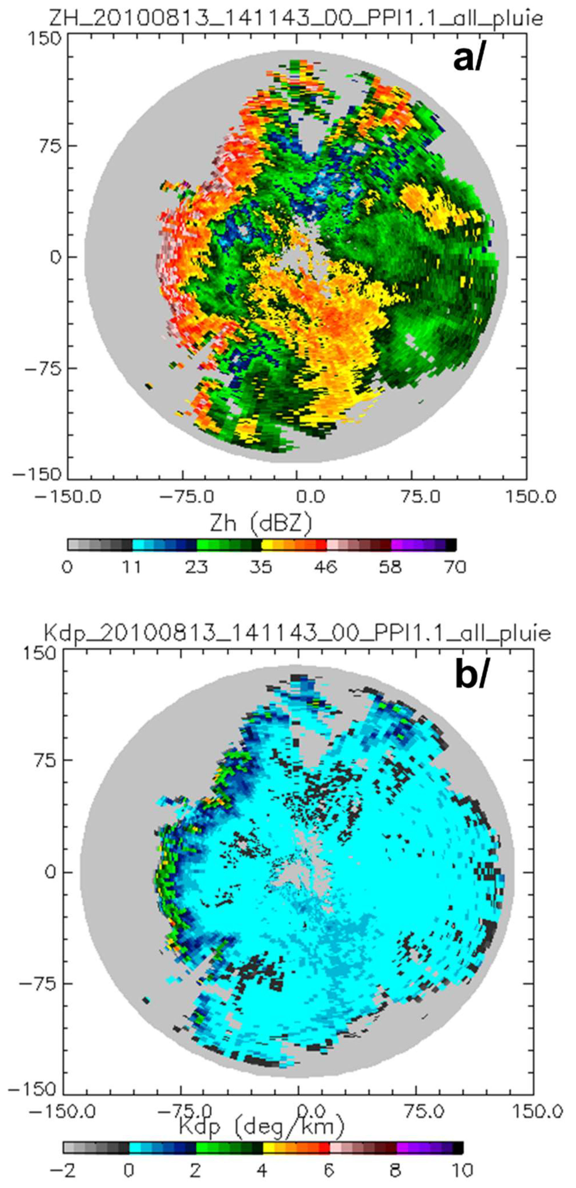
3.1. Original Datasets and Methodology

To implement the copula method introduced in the present study, two types of datasets were used. A set of synthetic polarimetric radar variables derived from simulations based on the T-matrix scattering code [63] was used to intrinsically illustrate the different steps involved in investigating the dependence between two variables, K_DP and R, within the copulas theory. For this purpose, a large sample of 11,647 one-minute DSDs was used as the basis for these electromagnetic scattering simulations, as detailed in the work of Gosset et al. [8]. The final objective was the application of the copula method to realistic radar data for quantitative precipitation estimation; R-K_DP algorithms were developed from copula simulations resulting from original datasets based on the X-band radar dataset (Xport) gathered during African Multidisciplinary Monsoon Analysis (AMMA) campaigns in the North of Benin [7,8,29]. This served to include measurement issues in investigating the dependence between K_DP and R throughout copulas theory. The performances of copula-based rainfall algorithms were assessed using measurements from the Xport experiment as part of the Megha-Tropiques algorithm validation campaign in Niamey (Niger) in August 2010 [64,65]. Sample PPI plots from the 13 August 2010 storm are presented in Figure 1. The plots show Xport reflectivity and specific differential phase fields. The radar rain rate estimates were compared with the network data of about 50 rain gauges. With this original approach, the robustness of the algorithms was thus evaluated.

3.2. Copulas Simulations Datasets

To illustrate the applicability of the copula simulation algorithms proposed in this paper, we considered the bivariate case including the rain rate R and the specific differential phase shift K_DP variables. The design of a synthetic database from the copula simulation results from a multi-step process that is thoroughly described by Genest and Favre [51] for a bivariate case study. Here, we outline the main steps. First, graphical methods were used to verify the link and the nature of dependency relationship between R and K_DP. One of the graphical tools used here to check for the existence of dependency is chi-plots [51]. This method was originally proposed by Fisher and Switzer [66,67]. Briefly, chi-plots are a construction based on the ${\chi }^2$ statistic to analyze the independence of samples in a two-way table from functions depending exclusively on the ranks of ‘observations’ (i.e., K_DP synthetic sample and rain rate R data from DSD measurements, as described above). For more details, the reader is referred to Genest and Favre [51].

The second step concerns the determination of the selected copula parameters, θ. As we mentioned above, this is achieved using a two-step method called IFM. The initial step consists of determining the appropriate margins for each concerned variable. To model the parametric distribution for univariate data, we used the method of maximum likelihood detailed in Section 2 using relation (16). To this end, we evaluated almost twenty theoretical distribution functions with one, two or three parameters, including Exponential, Geometric, Poisson, Rayleigh Weibul, Birnbaum-Saunders, Extreme Value, Gamma, Inverse Gauss, Logistics, Log-Logistic, Nakagami, Log-Normal, Normal, Rician, Uniform and Generalized Pareto distributions. The reason for using so many theoretical functions is that Genest and Favre [51] indicated that the IFM estimation copula parameter technique is sensitive to the selected theoretical marginal distribution. Therefore, it appeared useful to test a wide variety of functions and retain only those that best fit the empirical distributions of K_DP and R. The quality of the fit of marginal distributions was assessed using the criterion of Akaike (AIC criterion) suggested by Frees and Valdez [35]. This goodness-of-fit score was calculated for each theoretical distribution using the following formula:

$$AIC=n\times \log \left(MSE\right)+2\times k$$

(22)

where k is the number of parameters being estimated, which is determined by the type of univariate theoretical marginal distributions considered; $n$ is the size of the sampling dataset; and $MSE=\frac{{{\displaystyle \sum }}_{i=1}^n{\left[F_{th}\left(i\right)-F_{obs}\left(i\right)\right]}^2}{\mathrm{n}-1}$ represents the mean square error between the theoretical values ($F_{th}\left(i\right)$) and empirical distribution function values ($F_{obs}\left(i\right)$). Moreover, since it is a classical fact of statistics that the power of a test may depend on sample size, we also tested the effect of the ‘calibration’ data sample size.

Finally, the parametric estimates $F_{{\widehat{\alpha }}_1}$ and $F_{{\widehat{\alpha }}_2}$ of the margins were input to the log-likelihood of copula (Equation (17)), which was then maximized to determine the parameter $\theta$ of copula. These values of copula parameters were also estimated without assuming theoretical marginal distributions using the CML method. The advantages of using the two approaches is that $\theta$ determination from the IFM method could be assessed by comparing with the CML results and thus confirming the best margin theoretical functions.

3.3. Quantile Regression Method

One of the aims of this paper was to extend the observed dataset used for deriving rainfall estimators by adding synthetic extreme data from copula simulations which take into account the dependency between the considered variables. Because of the increased number of extreme values, regression techniques were required, which are less sensitive to those values than classic Least Mean Square estimation (hereafter LMS method) of rainfall algorithms. Indeed, for the conventional LMS method, the estimation of the mean parametric regression model μ(X, β) accounting for the dependence of the conditional mean of a variable Y on its covariates X is a solution for the minimizing problem

$$\beta =\underset{\beta }{\arg \min }{\displaystyle \sum }_{i=1}^n{\left(y_i-\mu \left(x_i,\beta \right)\right)}^2$$

(23)

where β stands for the parameters of the theoretical model μ(X, β), which is generally formulated as a linear function based on the logarithm transformation of variables Y and X in radar meteorology. In Equation (24), the minimized quadratic cost function increases quadratically with residuals, and very large differences should be penalized. Koenker and Hallock [68] indicated that the non-robustness of the LMS method is partially explained by the effect exerted by such unusual extreme values in the dataset. Furthermore, one of the limitations of the LMS regression method is to assume, a priori, that the explanatory variable X has a uniform effect on the whole distribution of the dependent variable Y. In our case, the variable of interest is the rainfall rate, which is characterized by strong variability and is highly dispersed. A specific value of K_DP corresponds to various values of rain rate. Lastly, the determination of algorithms for rainfall estimation is usually carried out using a given range of rainfall rate (variable interest). However, in such conditions when one observes the variable of interest beyond a threshold, estimation of the conditional mean and mean relationships is compromised in the presence of censored or truncated data [69].

The Quantile Regression Estimation (hereafter QRE) method provides a more detailed picture than the classic LSE method, as it focuses on the entire conditional distribution of the dependent variable, not only on its mean [68]. Givord and D’Haultfoeuille [69] argued that this method can be better adapted to certain types of data (truncated variables, presence of extreme values, non-linear models). According to the extensive discussion in Koenker and Hallock [68], QRE is based on minimizing asymmetrically weighted absolute residuals and is intended to estimate conditional median functions and a full range of other conditional quantile functions. In other words, in comparison to the LMS method of the mean regression model concerned with the dependence of the conditional mean Y on the explicative variable X, the quantile regression estimator tackles this issue at each quantile of the conditional distribution. Thus, the QRE method provides a more complete description of how the conditional distribution of Y given X = x depends on x. Moreover, quantile regressions are also better suited to truncated or censored dependent variables and the occurrence of extremes values in the dataset samples.

In brief, by considering the random variable Y, whose distribution function is expressed by $F_Y\left(y\right)=P\left(Y\le y\right)$, the p-th quantile of Y can be defined by:

$$Q_p\left(Y\right)=\mathrm{Inf}\left\{y: F_Y\left(y\right)\ge p\right\}$$

(24)

In the case of quantile regression estimators, the dependence of conditional quantiles of the variable of interest Y defined by Q_p(Y|X) = inf{y: F_Y|X(y) ≥ p}, with the explanatory variable X value, is modeled. In comparison with the LSE method based on the minimizing issue as written in Equation (24), the QRE method proceeds in exactly the same manner. However, the quantile regression is linked to the operations of ordering and sorting the observations [68]. From the ordered values, the estimation of the parameters β_p of the theoretical quantile function is realized by solving [68]:

$${\beta }_p=\arg \underset{\beta }{\min }{\displaystyle \sum }_{i=1}^n{\rho }_p\left(y_i-\xi \left(x_i, \beta \right)\right)$$

(25)

where ρ_p is a ’check function’ defined by ${\rho }_p\left(u\right)=u(p-\mathbb{I}(u<0))$, $\mathbb{I}$ is the usual indicator function, and $\xi \left(x_i,\beta \right)$ is the parametric function or the conditional quantile function.

Based on the works of Frees and Valdez [35] and Bouyé and Salmon [70], copulas are well suited to the concept of ‘quantile regression’. Specifically, in the case of bivariate parametric copula $C_{\theta }$, if the probability distribution of $y$ which is conditional on $x$ is defined by $p=F_Y\left(y|X=x\right)$, the p-th quantile would be the solution $y$ of the equation [35,70]:

$$p=F_Y\left(y|X=x\right)=C_1\left[F_X\left(x\right),F_Y\left(y\right),\theta \right]$$

(26)

where $C_1\left[u,v,\theta \right]=\frac{\partial }{\partial u}{C}_{\theta }$ is the first partial derivative for the considered copula, and $u=F_X$ and $v=F_Y$ are the distribution functions of the variables X and Y, respectively. Under certain conditions, if one is able to analytically express $C_1$, the partial derivative of the parametric copula $C_{\theta }$ and also analytically determine the inverse of this function, Bouyé and Salmon [70] reported that the quantile $y$ could be explicitly expressed as follows:

$$y=F_Y^{-1}\left[D\left(F_X\left(x\right), p, \theta \right)\right]$$

(27)

where $D\left(F_X\left(x\right), p, \theta \right)$ is the partial inverse of $C_1$.

Thus, for various quantiles and different values of x, Equation (27) results in regression curves that can be used directly for the estimates of Y values conditional on x. These curves might also be modeled by linear or nonlinear functions. However, such an approach is limited by the difficulty, for some parametric copulas, in determining an analytical expression for the inverse of the partial derivative $c_1$. Furthermore, in the case that $C_1$ is not analytically invertible, the procedure for numerical root finding may be computationally expensive. Hence, we determined the coefficients of rainfall algorithms by directly applying the above-mentioned method of ‘quantile regression’ on observed and copulas synthetic datasets.

4. Results

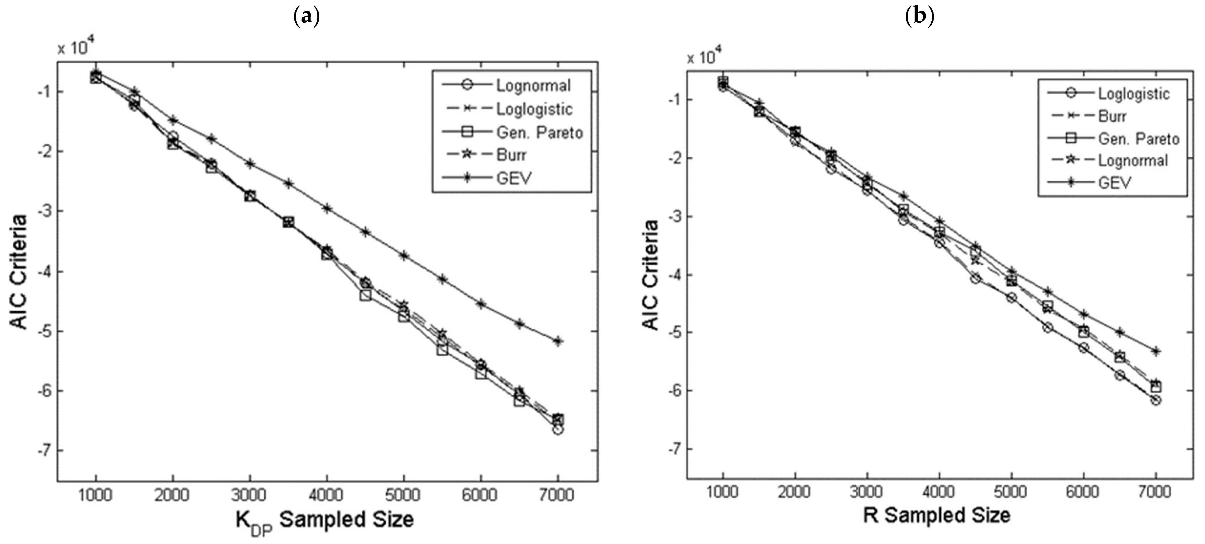
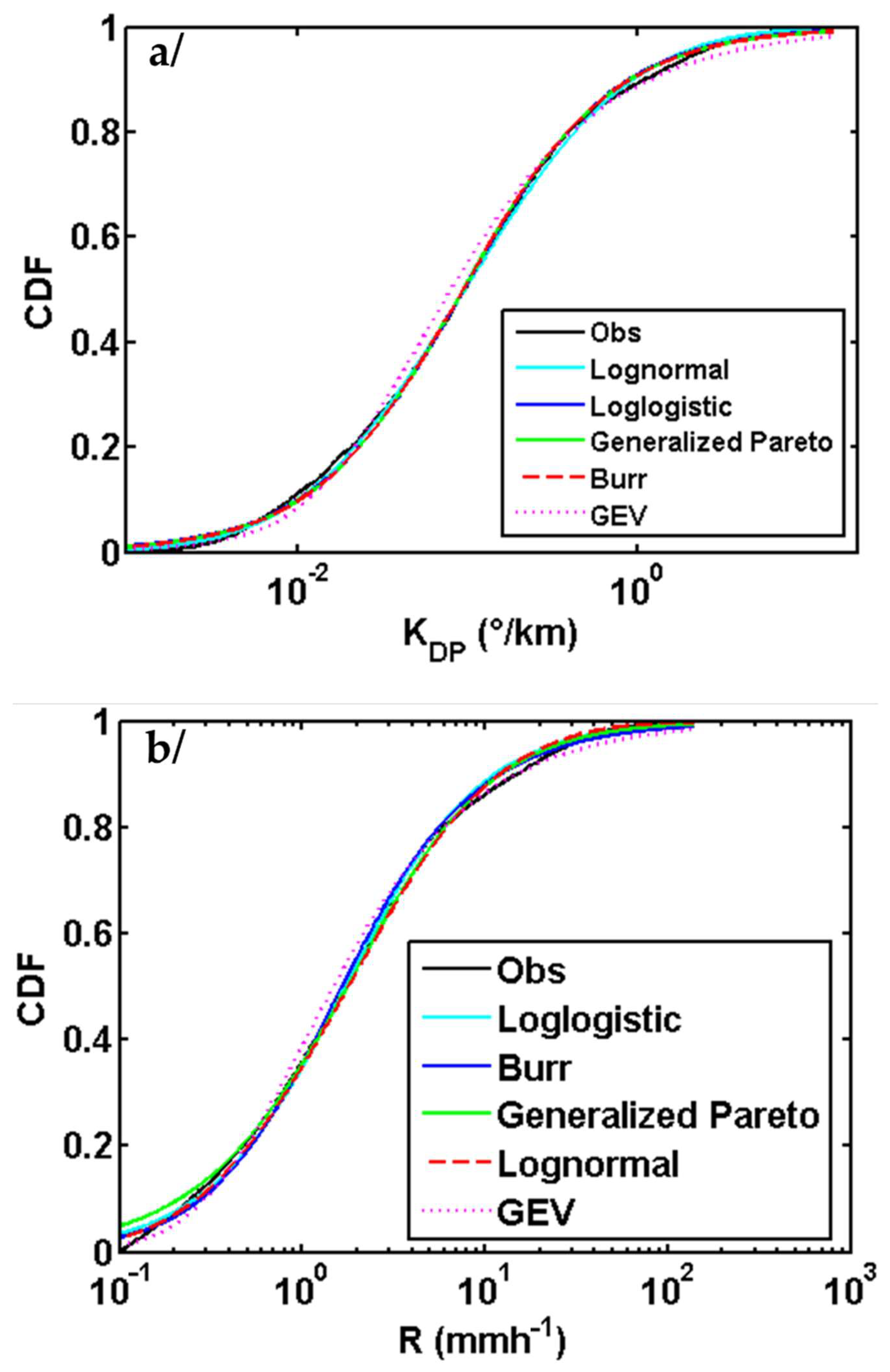
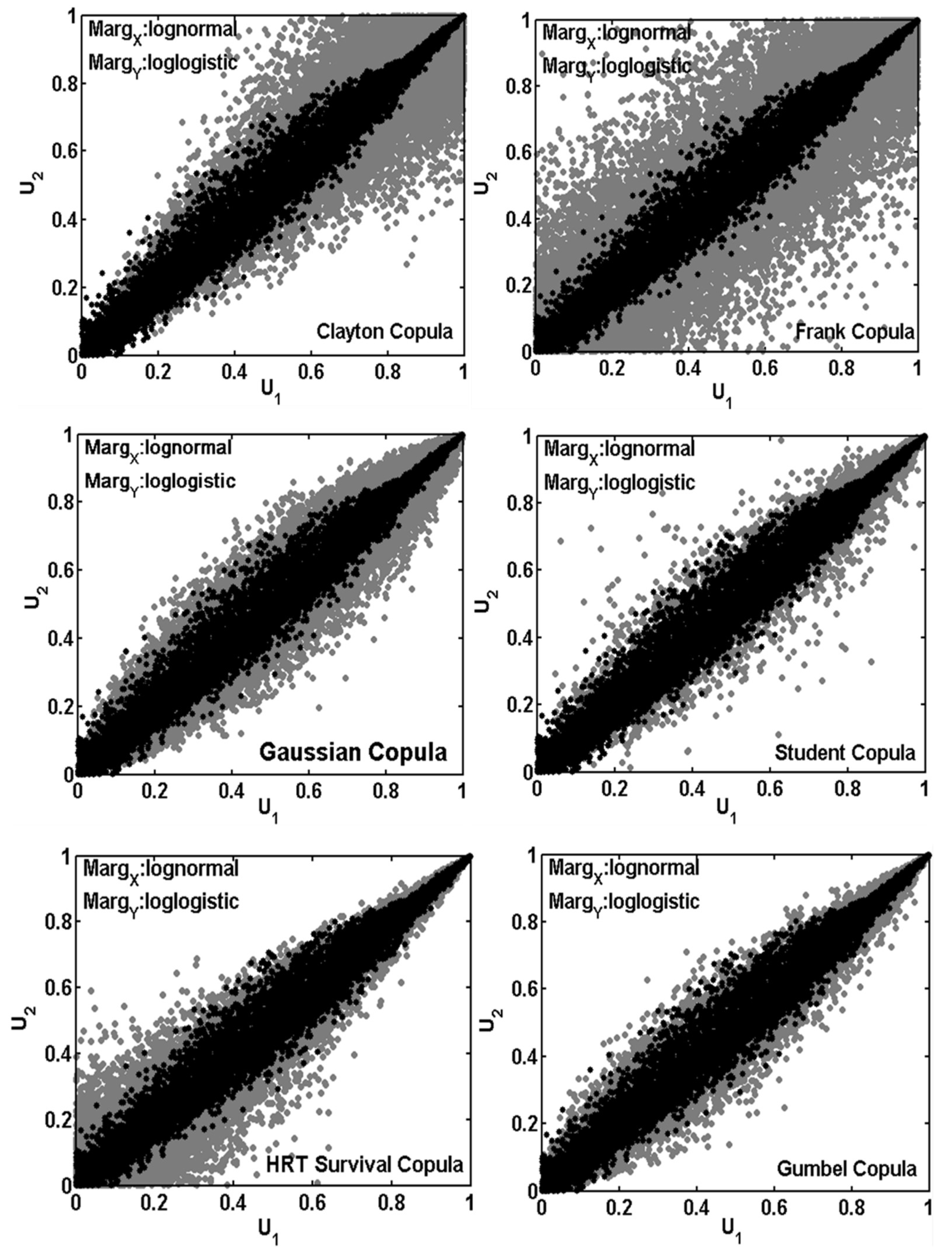
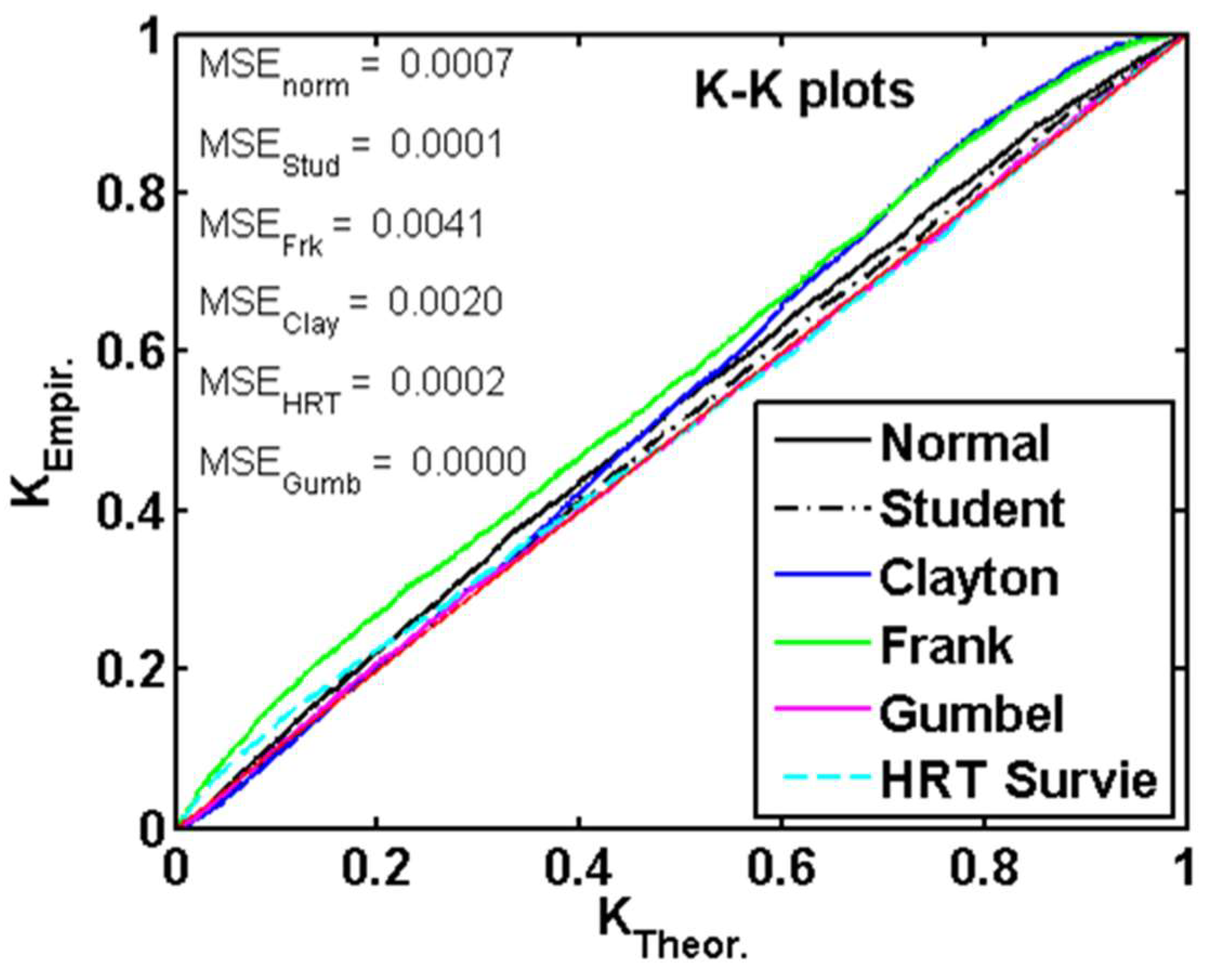
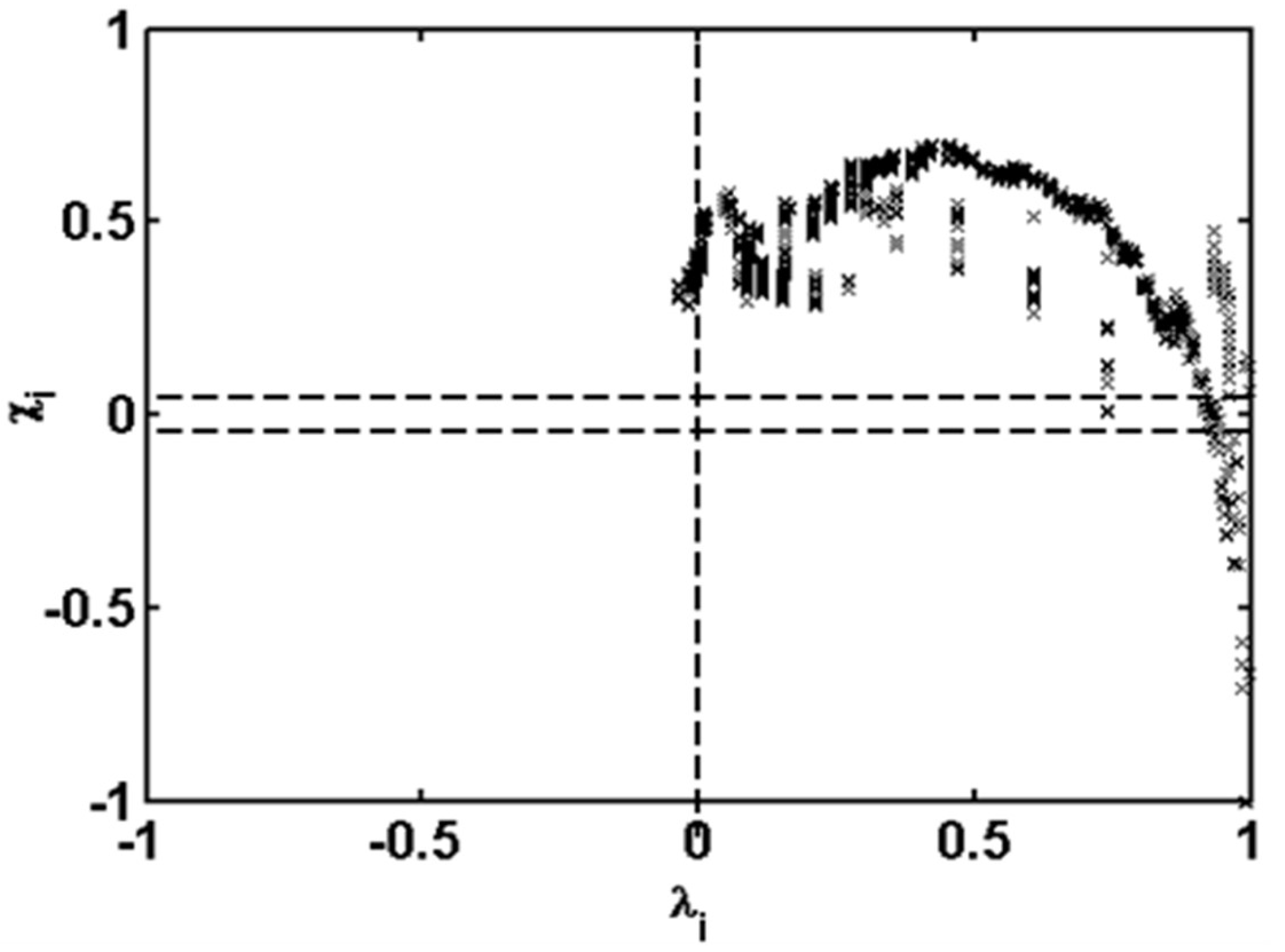
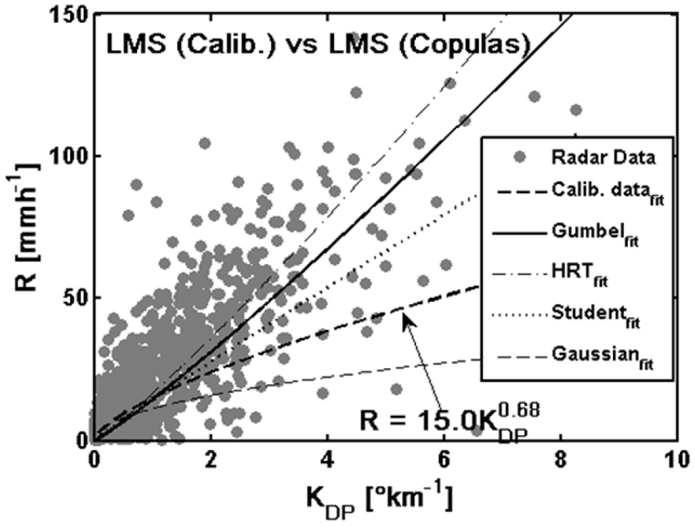
4.1. Copulas Simulation Datasets Assessment

Figure 2 shows the ‘chi-plot’ resulting from the sample of ‘calibration’ selected for K_DP and R variables. The coordinates of the points are $\left({\lambda }_i,{\chi }_i\right)$, where ${\lambda }_i$ is a measure of distance between the pair (K_DP⁽ⁱ⁾, R⁽ⁱ⁾) of the ‘calibration’ dataset and the center of the scatter plot and ${\chi }_i$ is the square root of the traditional chi-square test statistic for independence in the two-way table generated by counting points in the four regions delineated by the lines x = K_DP⁽ⁱ⁾ and y = R⁽ⁱ⁾ [51].

From Figure 2, it can be seen that most of the points do not fall (only one point) within the confidence band of the ‘chi-plot’ (delineated by dashed horizontal lines in the graph), which brings together the points indicating independency between the K_DP and R variables. As expected, we also noted the presence of a positive association between K_DP and R. To quantify the degree of dependence between K_DP and R, the empirical value of Kendall’s tau was calculated from relation (5). Based on the synthetic sample of K_DP and the DSD-derived rain rate, we obtained a value of 0.817, which indicated a good correlation between the two variables of interest.

Figure 3 shows, for the five best fitted theoretical distribution functions, the evolution of the AIC score as a function of the data sample size. The smallest AIC value indicates the best fitted model. One can readily see from Figure 3 the strong dependence of the test on sample size. For each variable, we retained only the model with the best AIC scores regardless of the sample size. Thus, the specific differential phase shift was modeled using the Generalized Pareto distribution, whereas the log-logistic distribution fits the original datasets of rain rates well. Figure 4 illustrates the empirical cumulative distribution function (CDF) of the variables R and K_DP for its five best theoretical distribution functions. It can be seen that despite the proximity of the CDF curves, the AIC criterion appears as a goodness-of-fit score for discrimination between them.

For all the selected copulas $C_{\theta }$, the obtained values of $\theta$ from the IFM method can be seen in

Table 3. Inference Function for Margins (IFM) and empirical Canonical Maximum Likelihood (CML) estimates of copula parameters from a sample of size 7000 of synthetic R and K_DP values from T-matrix simulations using DSD gathered at Nangatchori (Benin) during AMMA experiments. For IFM estimates, log-normal and log-logistic marginal functions were used for R and K_DP, respectively.

Copula	${\widehat{\mathit{\theta }}}_{\mathit{I}\mathit{F}\mathit{M}}$	${\widehat{\mathit{\theta }}}_{\mathit{C}\mathit{M}\mathit{L}}$
Clayton	7.728	6.574
Frank	9.620	9.678
HRT (Survival Clayton)	11.001	13.287
Gumbel	8.552	9.251
Normal (Gaussian)	0.983	0.980
Student’s	0.984 $\left(\nu =7\right)$	0.983 $\left(\nu =3\right)$

. These values of copula parameters were also estimated without assuming theoretical marginal distributions using the CML method. The proximity of the $\theta$ values, regardless of the estimation method, confirms the choice of K_DP and R margin theoretical distribution functions. Hereafter, only the values from the IFM method were considered.

Obviously, all the copulas are not appropriate and we should refine them using tools such as a dependogram, Kendall diagram or others existing in the literature. In our case, to test whether a copula is suitable for the description of the dependency in the data of interest, we compared the scatter plot of empirical uniform variables of K_DP and R (the empirical joint distribution function or copula) with the simulated dataset from copulas. This type of diagram is called a dependogram. Figure 5 shows examples of dependograms standing for the more or less simultaneous nature of the copula achievements with those of the empirical copula. This simultaneity (superimposition of black and gray dots) is more obvious for Gumbel and Student’s copulas, which would indicate a better characterization of the dependence between radar-specific differential phase shifts and rain rates by both theoretical copulas. In particular, in the tails, it will be useful to analyze whether concurrency is high and, therefore, if it is necessary to calibrate for our base sample a copula with tail dependence. For the Student’s copula, as expected, dependencies in the upper and bottom tails are because this copula is the only one to have non-zero asymptotic dependence for both small and large values. However, the Gumbel copula and HRT seem more suited to modeling the upper tail dependencies, while the Clayton copula is more appropriate for lower tail distributions.

One of the issues with using the copula method is selecting the copula that provides the best fit to resolve the problem at hand. Many proposals of goodness-of-fit tests for copulas exist in the literature [71,72]. However, since we have the possibility to determine the empirical copula of the data, the best copula could be chosen as the one that minimizes the distance to the empirical. This is realized using the K-K plot (Figure 6) derived from pseudo-samples obtained by transforming the empirical or original simulating data using the empirical distribution function (U₁ and U₂ for a bivariate case). The distance between the empirical and simulated copula is shown in the figure as the mean standard error (MSE) for each copula considered.

For the application and in order to include measurement issues, we considered actual specific differential phase shift (K_DP) from an X-band radar dataset gathered during AMMA experiments (2006–2007) in Northern Benin and the corresponding rain rates (R) using a rain gauges network operating during these campaigns. From a bivariate observed sample of size 2688, drawing a positive dependence between K_DP and R (Figure 7), we simulated 20,000 synthetic data samples following the simulation setup for the four best copula families (Gaussian, Student’s, Gumbel and HRT copulas) with parameters estimated by the IFM (Inference of Margins) method (

Table 4. Inference Function for Margins (IFM) and empirical Canonical Maximum Likelihood (CML) estimates of copula parameters from a sample of size of 2688 derived from areal data of R (rain gauges) and K_DP (Xport radar) operated in Northern Benin during AMMA experiments. For IFM estimates, GEV and Burr marginal functions were used for R and K_DP, respectively.

Copula	${\widehat{\theta }}_{IFM}$	${\widehat{\theta }}_{CML}$
Clayton	1.165	1.526
Frank	11.474	11.474
HRT (Survival Clayton)	3.084	2.682
Gumbel	2.616	2.601
Normal (Gaussian)	0.754	0.790
Student’s	0.793 $\left(\nu =2\right)$	0.816 $\left(\nu =3\right)$

). In Figure 8, observed couples (in black circles) are shown together with synthetic samples (gray circles). As expected, in the context of our application, synthetic datasets from copulas with non-null upper tail dependence (Gumbel, HRT and Student’s copulas) were close to the observed data values. In particular, they reproduce higher values than Gaussian copula simulations. This suggests the possibility of designing polarimetric rainfall algorithms for X-band radars since these realistic synthetic data involve large samples of higher values of K_DP and R.

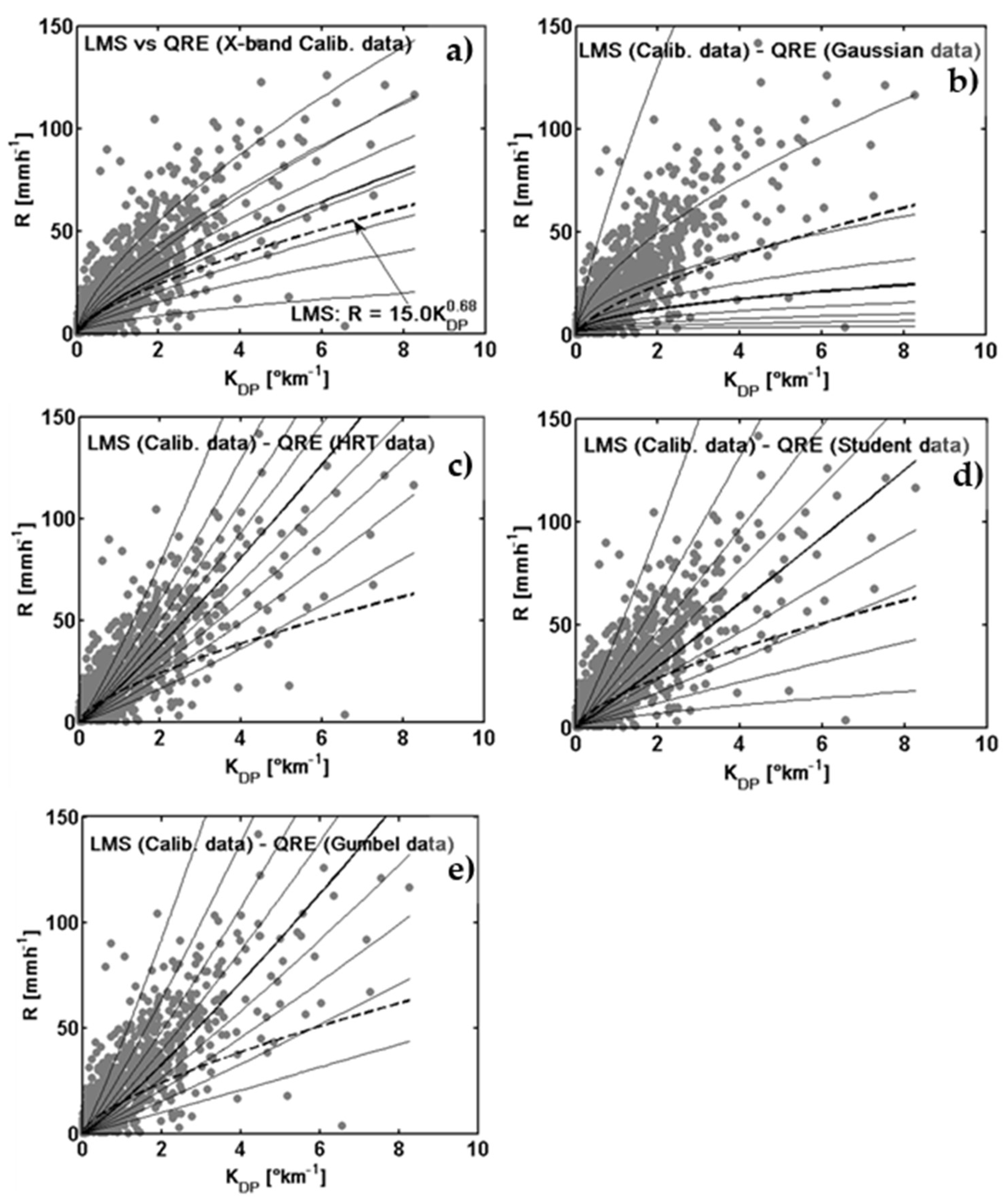
4.2. Statistical Rainfall Regression Estimators

For radar quantitative precipitation estimation to perform well, the convenient choice of algorithm is decisive. Thus, to analyze the impact of the datasets generated by the copula method, these data were used to determine the power-law algorithms $R=a{K}_{DP}^b$ by employing the classic LSE method. Each copula synthetic datasets were used to derive an equation for mean rain rate estimation. As a comparison, the Least Mean Square estimate (LMS) based on an observed ‘calibration’ dataset was also performed. Figure 9 illustrates the difference between the derived algorithms by superimposing on the scatterplot of R-K_DP observed data (gray points), the fitting curves from copula datasets and the resulting rainfall algorithms based on the original database. We also show the relation of the LMS method based on ‘calibration’ data without thresholds, which differs from the estimator derived by Koffi et al. [29] that discarded rain rates of below 5 mm/h, whereas in the present study, we considered the entire range of rain rates.

The algorithms from extreme values of Gumbel copula and that of Student’s copula (which has no null asymptotic upper tail dependence coefficient) fit well with the observed dataset. The copula approach can help to correct the disadvantages due to the lack of sufficient extreme values in the database of previous investigations. Moreover, the fact that the algorithm from the Gaussian copula (or bivariate normal copula), which is not an extreme values model, performs better than the classic R-K_DP derived directly from ‘calibration data’ indicates the usefulness of the copula approach, which allows us to better characterize the dependency between variables in relationships by using invariant data logarithm transformation correlation coefficients.

The further analysis of LMS together with QRE-based rainfall algorithms is subsequently presented in Figure 10 with the aim of showing the potential improvement of fitting by taking into account quantile regression estimation. From Quantile Regression Estimation (QRE) and LMS-derived algorithms, there is evidence that there is a gap between the LMS mean fitted curve and the 0.5 quantile adjustments. As mentioned above, this is partially due to the non-robustness of the LMS method that is affected by the effect exerted by unusual extreme values in the dataset [68]. This gap appears to increase when considering extreme value copulas, as Gumbel and HRT show uneven fitting results for 0.5 quantile conditional distributions relative to LMS regression. In addition, according to the copula considered, adjusted R-K_DP curves are qualitatively better for quantiles above 0.5. For Gaussian copula, to achieve the best performing algorithm, we should consider 0.8 percentile distribution. Conversely, lower percentiles are better for Student’s, Gumbel and HRT copula estimators. This highlights the need to investigate the entire conditional distribution to determine radar rainfall estimators.

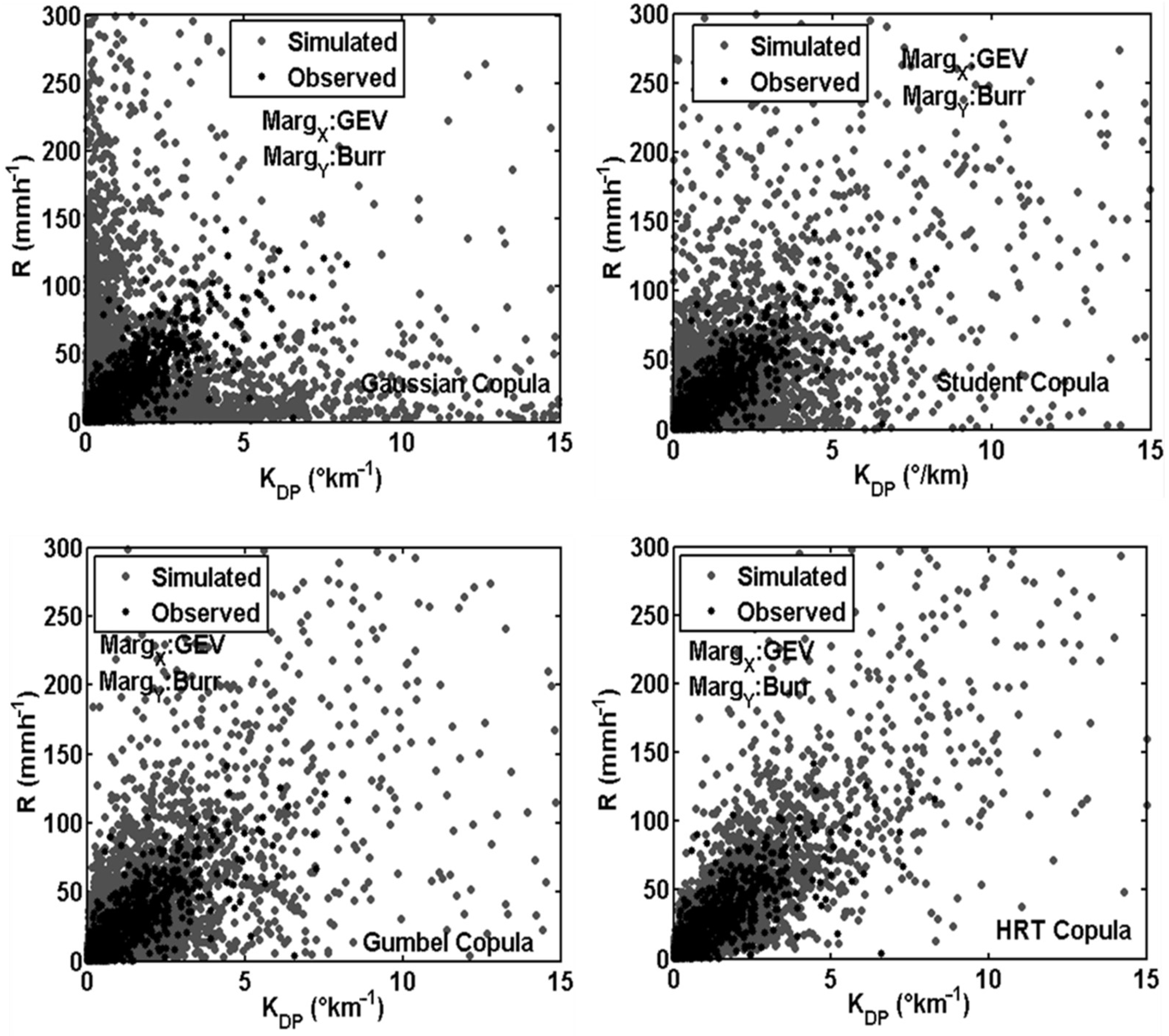
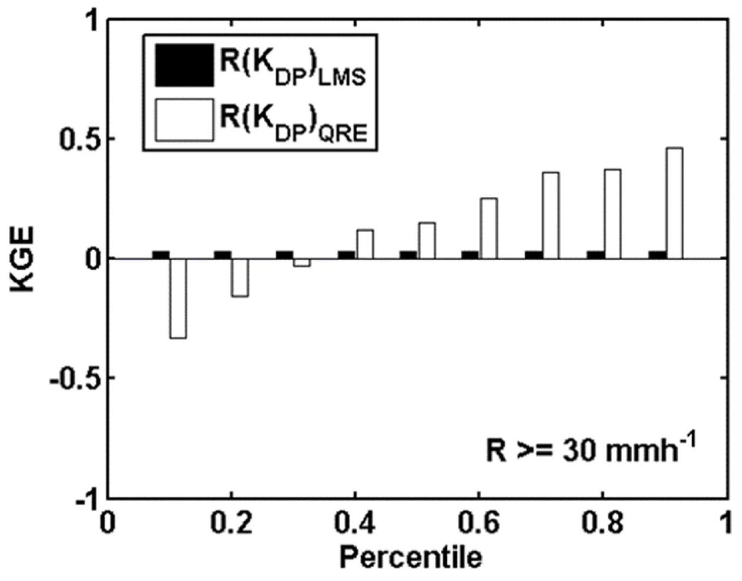
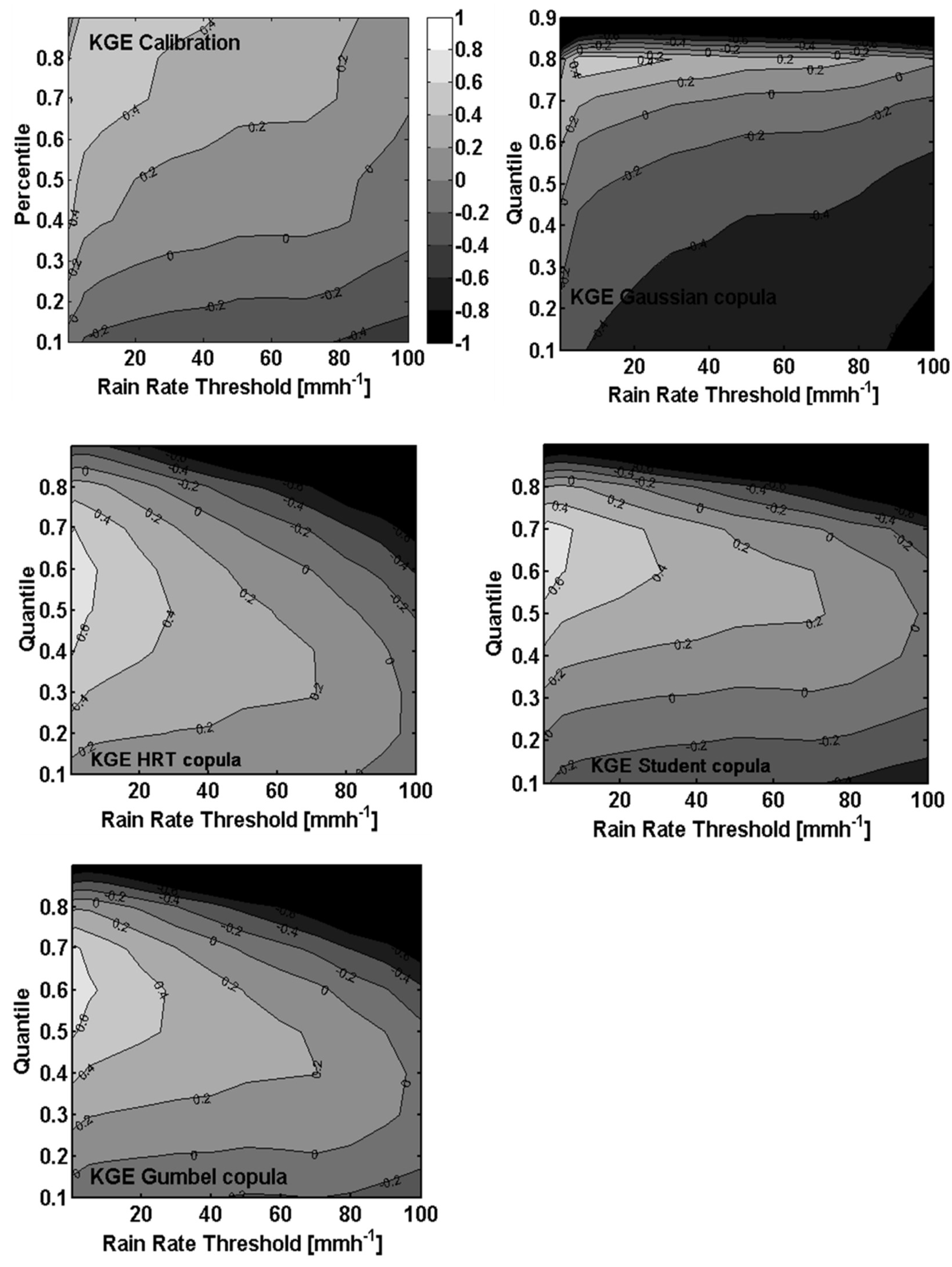
4.3. Evaluation of Rainfall Estimation

The performances of the rainfall estimation algorithms applied to K_DP values from the ‘validation’ sample (data from X-band experiments in Niamey in 2010) were quantitatively evaluated by comparing retrievals to rain rate of the same sample using bulk statistics for intense rain rates (R ≥ 30 mm/h), often poorly retrieved (Figure 11). As expected from Figure 9, in heavy rain situations, the performance of the classic R(K_DP) algorithm from the LMS method was four times less than the 0.5 percentile-derived algorithm. Rain rates of over 30 mm/h yield increased the performance of estimators with the percentile considered. Thus, the 0.9 percentile-derived R(K_DP) is the best estimator with a Kling and Gupta efficiency (KGE) [73] of 12 times higher than Least Mean Square method.

The impact of the copula approach was also quantitatively studied. Figure 12 displays the performance of algorithms investigated by stratifying results according to various thresholds on the rain gauge rates and involving whole data distribution with respect to the percentile of rainfall rates considered to determine algorithms. The KGE score is used to measure how close estimations are to the observations. To better understand the interpretation of results, it is useful to keep in mind that a value of 1 indicates perfect estimates, while a KGE value equal to 0 or negative means the retrieval is not better or even worse, respectively, than using the mean value of predicted rain rates.

It is evident from the figure that for a given rainfall rate threshold (lower bound of the considered rainfall rate interval) indicating the targeted rainfall type for radar retrieval, the R(K_DP) estimator becomes more efficient considering larger K_DP-conditioned rainfall quantiles for the determination of its coefficients based on radar/rain gauge data samples. A similar result is also observed for R(K_DP) algorithms based on Gaussian copula simulations for quantiles up to 0.7. However, between quantiles 0.7 and 0.8, it was exhibited that the KGE values (standing for the performance of estimator) are independent of the quantile considered for a targeted rainfall type.

On the other hand, for the retrieval of a specific type of rainfall from the radar, the estimators deduced from HRT, Gumbel and Student’s copulas show a greater independence from the quantile considered for its determination. This result indicates that such algorithms are more robust with respect to the choice of K_DP-conditioned rainfall quantiles considered when establishing them.

For heavy rainfall rates (>30 mm/h), algorithms derived from synthetic Gumbel, Student’s, HRT and Gaussian simulated datasets exhibited better performance compared to the retrieval method based on ‘calibration’ observed radar and rain gauge datasets. Specifically, for the percentile range from 0.2 to 0.8, algorithms derived from Gumbel, Student’s and HRT copulas with non-null tail distributions led to a KGE of above 0 for a rain rate threshold of almost 100 mm/h. This result shows that copula-based R(K_DP) algorithms lead to better performance than the classic method based on radar-gauge comparison for rain rates higher than 100 mm/h. Thus, to reach such a performance, a Gaussian-derived algorithm should be determined considering percentiles between 0.6 and 0.8. The reason would be that the Gaussian copula with a null tail distribution is unable to reliably reproduce rain rates and specific differential phase extreme values, as shown in Figure 8.

5. Discussion and Conclusions

Quantitative precipitation estimates (QPE) by weather radar suffer from several sources of uncertainties that are often difficult to disentangle. Very often, the poor representation of the links between radar observables and rainfall parameters such as rain rate, especially for intense rainfall, which is insufficiently represented in the adjustment samples of rainfall estimators, limits its performance. The optimization methods of algorithms based on setting up estimators by focusing on specific ranges of rainfall may prove to be ineffective when applied for the retrieval of other types of rain rates outside the calibration rainfall range considered. Furthermore, the generally used statistical method for determining the algorithms based on Least Mean Squares may be inadequate when it comes to investigating the whole distribution of variables targeted for establishing the rainfall estimators.

In this study, we proposed a method for estimating rainfall rates through the R(K_DP) algorithm, whose coefficients were determined from simulations of extreme value copulas, allowing us to transcribe the link between R and K_DP for all rain types. This approach explicitly accounts for the joint empirical distributions of these two variables that are modeled by the well-chosen copulas. To evaluate the robustness of the method, the algorithms were fitted based on radar/gauge data of events gathered during the AMMA intensive campaign in Northern Benin in 2007 and applied to the events in Niamey observed during the validation experiment of Megha-Tropiques satellite measurements in 2010.

By conducting a quantitative diagnosis in terms of the KGE performed for rain rates of greater than 30 mm/h for algorithms based only on radar/gauge observed ‘calibration’ dataset (LMS and QRE statistical methods applied to derive R(KDP) coefficients), conditional quantile regression algorithms significantly reduced the errors in rainfall retrieval, more so than LMS regression. It was shown that assuming a 0.9 percentile, KGE increases to 0.5, a score that is rarely achieved for this type of rain. The similarity score for the R(K_DP) algorithm has been reported by researchers [29,74] in the optimizing framework of the performances of this estimator. To reach such scores, in the cited previous work, all rainfall types were included in the bulk statistics. Given the high weight of rainfall rates below 30 mm/h, their results were more influenced by this range of rainfall. Unlike these works, in our study, only higher intensity rainfalls (>30 mm/h) were considered for the KGE calculation, whereas for these rain types, the performance of the algorithms was generally degraded. Thus, it was shown that Quantile Regression Estimation performs better than the Least Mean Square method that assumes the mean distribution.

Another interesting result that is clearly shown in this study is the contribution of the copula approach to increasing the performance of algorithms in estimations of the higher intensity rain rates. At this stage, R(K_DP) formulas were fitted using either copula-simulated datasets or radar/gauge observations by applying only Quantile Regression Estimation. We noticed that the R(K_DP) estimator adjusted for radar/rain calibration does not exceed 0.6 in terms of KGE regardless of the percentile and rainfall rate threshold considered. In addition, the reliable determination of intense rainfall (>30 mm/h) is almost impossible considering R(K_DP) algorithms pre-established by considering sample quantiles of calibration data of less than 0.3. For higher rainfall rates (i.e., for higher thresholds considered to describe extreme rainfall), more important quantiles must be considered for the establishment of algorithms in order to lead to reliable estimates. For this purpose, Matrosov et al. [27,28] and Koffi et al. [29] used the traditional LMS method that is closest to the 50th quantile (a measure of the central tendency of the distribution) to achieve satisfactory results for rainfall greater than 30 mm/h. However, as we can see in the current work, this is a minimum threshold since the QRE method shows that better performance can be achieved by considering higher quantiles for the same types of targeted precipitation rates. Thus, it was found that rainfall corresponding to higher quantiles provides more accurate estimates of intense precipitation. With a QRE method, users are free to choose the desired statistical quantile level according to their application [49].

For estimators derived from simulated extreme value copulas (Gumbel and HRT) or with non-null distribution tail copulas (Student’s copula), the errors are considerably reduced, with the possibility of obtaining a performance score (KGE) varying between 0.6 and 0.8 for rainfall rates of above 5 mm/h. These results are all the more important as they overpass those of Koffi et al. [29], although they applied optimization criteria (giving more weight to higher rain rates by discarding values below 5 mm/h) when determining the coefficients of the R(K_DP) estimator, contrary to our results, for which no thresholding on rain rate values were obtained a priori. Moreover, at equal percentiles between 0.15 and 0.8, the estimators derived from the synthetic copula data outperformed those derived from the radar/gauge observations. This indicates that taking into account the link between the radar (K_DP) and rainfall (R) variables is crucial for better-performing algorithms. The knowledge of such a link is even more important for acceptable retrievals of heavy rainfall. Our results show that for the Gumbel, HRT and Student’s copulas, given percentiles between 0.2 and 0.8, it appears possible to adequately estimate rainfall rates of almost above 100 mm/h (KGE > 0). For a Gaussian copula, reaching such performances requires considering higher percentiles (0.6 to 0.8) for estimators’ determination. This demonstrates, first, the importance of taking into account tail dependence copulas (HRT, Gumbel and Student’s) in the context of extreme rainfall quantitative estimation. The algorithms for estimating intense rainfall based on such copulas of extreme values (HRT and Gumbel) and those with non-zero tail distribution (Student’s) to a lesser degree are better suited and more robust since their performances seem, in terms of KGE, not to be dependent on the choice of the rain rate range (standing by a wide range of percentile values from 0.2 to 0.8 providing similar KGE scores) considered for their determinations. These results illustrate the interest of including the copula approach in the design of QPE algorithms. In particular, to overcome the limitation in the size of the calibration datasets and scarcity of extreme values, which are drawbacks in determining efficient rainfall estimators of intense precipitations, the copula method appears quite important to generate reliable synthetic datasets. This study highlighted the advantage of using a copula model that captures the dependence between radar observable and rainfall parameters and consequently offers a way to produce accurate simulations of extreme rainfall. Furthermore, the Quantile Regression Estimation method, applied on such synthetic datasets, provides a more detailed picture than the classic LMS method as it focuses on the entire conditional distribution of the dependent variables, not only on its mean. In future work, a promising approach using copulas that we should consider is probabilistic quantitative precipitation estimation by directly inverting, analytically or numerically, the first partial derivative of the considered parametric copula. Such a method would allow us to discard the assumption of a power-law relationship between R and K_DP. Moreover, monitoring the probability of extreme precipitation leading to flash flooding could be achieved by combining this method with pre-established precipitation rate thresholds.

References

1. Chapon, B.; Delrieu, G. Variability of rain drop size distribution and its effect on the Z-R relationship: A case study for intense Mediterranean rainfall. Atmos. Res. 2008, 87, 52–65. [Google Scholar] [CrossRef]
2. Zawadzki, I. Factors Affecting the Precision of Radar Measurement of Rain. In Proceedings of the 22th Conference on Radar Meteorology, AMS, Zurich, Switzerland, 10–13 September 1984; pp. 251–256. [Google Scholar]
3. Pellarin, T.; Delrieu, G.; Saulnier, G.-M.; Andrieu, H.; Vignal, B.; Creutin, J.-D. Hydrologic Visibility of Weather radar systems operating in mountainous regions: Case study for the Ardèche Catchment (France). J. Hydrometeor. 2002, 3, 539–555. [Google Scholar] [CrossRef]
4. Steiner, M.; Smith, J.; Uijlenenhoet, R. A microphysical interpretation of Radar Reflectivity-Rain rate relationships. J. Atmos. Sci. 2004, 61, 1114–1131. [Google Scholar] [CrossRef]
5. Lee, G.W.; Zawadzki, I. Variability of drop size distributions: Time-scale dependence of the variability and its effects on rain estimation. J. Appl. Meteorol. 2005, 44, 241–255. [Google Scholar] [CrossRef]
6. Berne, A.D.; Uijlenenhoet, R. A stochastic model of range profiles of raindrop size distributions: Application to radar attenuation correction. Geophys. Res. Lett. 2005, 32. [Google Scholar] [CrossRef]
7. Moumouni, S.; Gosset, M.; Houngninou, E. Main features of rain drop size distributions observed in Benin, West Africa, with optical disdrometers. Geophys. Res. Lett. 2008. [Google Scholar] [CrossRef]
8. Gosset, M.; Zahiri, E.-P.; Moumouni, S. Rain drop size distribution variability and impact on X-band polarimetric radar retrieval: Results from the AMMA campaign in Benin. Q. J. R. Meteorol. Soc. 2010, 136, 243–256. [Google Scholar] [CrossRef]
9. Ochou, A.D.; Zahiri, E.-P.; Bamba, B.; Koffi, M. Understanding the variability of Z-R relationships caused by natural variations in raindrop size distributions (DSD): Implication of drop size and number. Atmos. Clim. Sci. 2011, 1, 147–164. [Google Scholar] [CrossRef]
10. Bamba, B.; Ochou, A.D.; Zahiri, E.-P.; Kacou, M. Consistency in Z-R relationship variability regardless precipitating systems, climatic zones observed from two types of disdrometer. Atmos. Clim. Sci. 2014, 4, 941–955. [Google Scholar] [CrossRef]
11. Sauvageot, H.; Lacaux, J.P. The shape of averaged drop size distributions. J. Atmos. Sci. 1995, 52, 1070–1083. [Google Scholar] [CrossRef]
12. Tokay, A.; Short, D.A. Evidence from tropical raindrop spectra of the origin of rain from stratiform versus convective clouds. J. Appl. Meteorol. 1996, 35, 355–371. [Google Scholar] [CrossRef]
13. Yuter, S.E.; Houze, R.A. Measurements of raindrop size distribution over the pacific warm pool and implementations for Z-R relations. J. Appl. Meteorol. 1997, 36, 847–867. [Google Scholar] [CrossRef]
14. Tenorio, R.S.; Moraes, M.C.S.; Sauvageot, H. Raindrop size distribution radar parameters in coastal tropical rain systems of northeastern Brazil. J. Appl. Meteorol. Clim. 2012, 51, 1960–1970. [Google Scholar] [CrossRef]
15. Campos, E.; Zawadzki, I. Instrumental Uncertainties in Z–R Relations. J. Appl. Meteorol. 2000, 39, 1088–1102. [Google Scholar] [CrossRef]
16. Bringi, V.; Rico-Ramirez, M.; Thurai, M. Rainfall estimation with an operational polarimetric C-band radar in the United Kingdom: Comparison with a gauge network and error analysis. J. Hydrometeor. 2011, 12, 935–954. [Google Scholar] [CrossRef]
17. Hasan, M.M.; Sharma, A.; Johnson, F.; Mariethoz, G.; Seed, A. Correcting bias in radar Z–R relationships due to uncertainty in point rain gauge networks. J. Hydrol. 2014, 519, 1668–1676. [Google Scholar] [CrossRef]
18. Dai, Q.; Yang, Q.; Zhang, J.; Zhang, S. Impact of gauge representative error on a radar rainfall uncertainty model. J. Appl. Meteorol. Clim. 2018, 57, 2769–2787. [Google Scholar] [CrossRef]
19. Steiner, M.; Houze, R.A., Jr. Sensitivity of the estimated monthly convective rain fraction to the choice of Z-R relation. J. Appl. Meteorol. Clim. 1997, 36, 452–462. [Google Scholar] [CrossRef]
20. Seliga, T.A.; Bringi, V.N.; Al-Khatib, H.H. A preliminary study of comparative measurements of rainfall rate using the differential reflectivity radar technique and a raingage network. J. Appl. Meteorol. 1981, 20, 1362–1368. [Google Scholar] [CrossRef]
21. Seliga, T.A.; Aydin, K.; Direskeneli, H. Disdrometer measurements during na intense rainfall event in central Illinois: Implications for differential reflectivity radar observations. J. Clim. Appl. Meteor. 1986, 25, 835–846. [Google Scholar] [CrossRef]
22. Gorgucci, E.; Scarchilli, G.; Chandrasekar, V. A robust estimator of rainfall rate using differential reflectivity. J. Atmos. Oceanic Technol. 1994, 11, 586–592. [Google Scholar] [CrossRef]
23. Gorgucci, E.; Chandrasekar, V.; Baldini, L. Rainfall estimation from X-band dual polarization radar using reflectivity and differential reflectivity. Atmos. Res. 2006, 82, 164–172. [Google Scholar] [CrossRef]
24. Jameson, A.R. A comparison of microwave techniques for measuring rainfall. J. Appl. Meteorol. 1991, 30, 32–54. [Google Scholar] [CrossRef]
25. Ryzhkov, A.V.; Zrnic, D.S. Comparison of dual-polarisation radar estimators of rain. J. Atmos. Oceanic Technol. 1995, 12, 249–256. [Google Scholar] [CrossRef]
26. Ryzhkov, A.V.; Zrnic, D.S. Assessment of rainfall measurement that uses specific differential phase. J. Appl. Meteor. 1996, 35, 2080–2090. [Google Scholar] [CrossRef]
27. Matrosov, S.Y.; Clark, K.A.; Martner, B.E.; Tokay, A. X-band polarimetric radar measurements of rainfall. J. Appl. Meteor. 2002, 41, 941–952. [Google Scholar] [CrossRef]
28. Matrosov, S.Y.; Kingsmill, D.E.; Martner, B.E.; Ralph, F.M. The utility of X-band radar for quantitative estimates of rainfall parameters. J. Hydrometeorol. 2005, 6, 248–262. [Google Scholar] [CrossRef]
29. Koffi, A.K.; Gosset, M.; Zahiri, E.-P.; Ochou, A.D.; Kacou, M.; Cazenave, F.; Assamoi, P. Evaluation of X-band polarimetric radar estimation of rainfall and rain drop size distribution parameters in West Africa. Atmos. Res. 2014, 143, 438–461. [Google Scholar] [CrossRef]
30. Bringi, V.N.; Chandrasekar, V.; Balakrishnan, N.; Zrnic, D.S. An examination of propagation effects in rainfall on radar measurements at microwave frequencies. J. Atmos. Oceanic Technol. 1990, 7, 829–840. [Google Scholar] [CrossRef]
31. Bringi, V.N.; Chandrasekar, V. Polarimetric Doppler Weather Radar: Principles and Applications; Cambridge University Press: Cambridge, UK, 2001; p. 636. [Google Scholar]
32. Zahiri, E.-P.; Gosset, M.; Lafore, J.P.; Gouget, V. Use of a radar simulator on the output fields from a numerical mesoscale model to analyse X-band rain estimators. J. Atmos. Oceanic Technol. 2008, 25, 341–367. [Google Scholar] [CrossRef]
33. Bouyé, E.; Durrleman, V.; Nikeghbali, A.; Riboulet, G.; Roncalli, T. Copulas for Finance a Reading Guide and Some Applications; Working Paper; Groupe de Recherche Operationnelle, Credit Lyonnais: Paris, France, 2000. [Google Scholar]
34. Embrechts, P.; McNeil, A.; Straumann, D. Correlation and Dependence in Risk Management: Properties and Pitfalls, in Risk Management: Value at Risk and Beyond; Cambridge University Press: Cambridge, UK, 2002; pp. 176–223. [Google Scholar]
35. Frees, E.W.; Valdez, E.A. Understanding relationships using copulas. N. Am. Actuar. J. 1998, 2, 1–25. [Google Scholar] [CrossRef]
36. Grimaldi, S.; Serinaldi, F. Asymmetric copula in multivariate flood frequency analysis. Adv. Water Res. 2006, 29, 1155–1167. [Google Scholar] [CrossRef]
37. Poulin, A.; Huard, D.; Favre, A.-C.; Pugin, S. Importance of tail dependence in bivariate frequency analysis. J. Hydrol. Eng. 2007, 12, 394–403. [Google Scholar] [CrossRef]
38. Tianyuan, L.; Guo, S.; Chen, L.; Guo, J. Bivariate flood frequency analysis with historical information based on copula. J. Hydrol. Eng. 2013, 18, 1018–1030. [Google Scholar] [CrossRef]
39. Favre, A.-C.; El Adlouni, S.; Perreault, L.; Thiémonge, N.; Bobée, B. Multivariate hydrological frequency analysis using copulas. Water Resour. Res. 2004, 40, 1–12. [Google Scholar] [CrossRef]
40. Salvadori, G.; De Michele, C. Frequency analysis via copulas: Theoretical aspects and applications to hydrological events. Water Resour. Res. 2004, 40, W12511. [Google Scholar] [CrossRef]
41. De Michele, C.; Salvadori, G.; Canossi, M.; Petaccia, A.; Rosso, R. Bivariate statistical approach to check adequacy of dam spillway. J. Hydrol. Eng. 2005, 10, 50–57. [Google Scholar] [CrossRef]
42. Hooshyaripor, F.; Tahershamsi, A.; Golian, S. Application of copula method and neural networks for predicting peak outflow from breached embankments. J. Hydro-Environ. Res. 2013, 8, 292–302. [Google Scholar] [CrossRef]
43. Shiau, J.T. Fitting drought duration and severity with two-dimensional copulas. Water Resour. Manag. 2006, 20, 795–815. [Google Scholar] [CrossRef]
44. Reddy, M.J.; Ganguli, P. Application of copulas for derivation of drought severity-duration-frequency curves. Hydrol. Process. 2012, 26, 1672–1685. [Google Scholar] [CrossRef]
45. Mirabbasi, R.; Fakheri-Fard, A.; Dinpashoh, Y. Bivariate drought frequency analysis using the copula method. Theor. Appl. Climatol. 2011, 108, 191–206. [Google Scholar] [CrossRef]
46. Vandenberghe, S.; Verhoest, N.E.C.; De Baets, B. Fitting bivariate copulas to the dependence structure between storm characteristics: A detailed analysis based on 105 year 10 min rainfall. Water Resour. Res. 2010, 46, W011512. [Google Scholar] [CrossRef]
47. Salvadori, G.; De Michele, C. Statistical characterization of temporal structure of storms. Adv. Water Res. 2006, 29, 827–842. [Google Scholar] [CrossRef]
48. Schölzel, C.; Friederichs, P. Multivariate non-normally distributed random variables in climate research—Introduction to the copula approach. Nonlin. Processes Geophys. 2008, 15, 761–772. [Google Scholar] [CrossRef]
49. Maity, R.; Dey, S.; Varum, P. Alternative approach for estimation of precipitation using Doppler weather radar data. J. Hydrol. Eng. 2015, 20, 04015006. [Google Scholar] [CrossRef]
50. Sklar, A. Fonctions de repartitions à n dimensions et leurs marges. Publ. Inst. Statist. Univ. Paris 1959, 8, 229–231. [Google Scholar]
51. Genest, C.; Favre, A.C. Everything you always wanted to know about copula modeling but were afraid to as. J. Hydrol. Eng. 2007, 12, 347–368. [Google Scholar] [CrossRef]
52. Schweizer, B.; Wolff, E. nonparametric measures of dependence for random variables. Ann. Statist. 1981, 9, 879–885. [Google Scholar] [CrossRef]
53. Nelsen, R.B. An Introduction to Copulas; Springer Lecture Notes in Statistics; Springer: New York, NY, USA, 1999; p. 139. [Google Scholar]
54. Fang, H.-B.; Fang, K.-T.; Kotz, S. The meta-elliptical distributions with given marginals. J. Multi. Anal. 2002, 82, 1–16. [Google Scholar] [CrossRef]
55. Genest, C.; MacKay, J. The joy of copulas: Bivariate distributions with uniform marginals. Am. Stat. 1986, 40, 280–283. [Google Scholar] [CrossRef]
56. Genest, C.; Rivest, L.-P. Statistical inference procedures for bivariate Archimedean copulas. J. Am. Statist. Assoc. 1987, 88, 1034–1043. [Google Scholar] [CrossRef]
57. Genest, C.; Ghoudi, K.; Rivest, L.-P. A semiparametric estimation procedure of dependence parameters in multivariate families of distributions. Biometrika 1995, 82, 543–552. [Google Scholar] [CrossRef]
58. Juri, A.; Wüthrich, M.V. Copula convergence theorems for tail events. Insur. Math. Econ. 2002, 24, 139–148. [Google Scholar] [CrossRef]
59. Juri, A.; Wüthrich, M.V. Tail dependence from a distributional point of view. Extremes 2004, 6, 213–246. [Google Scholar] [CrossRef]
60. Li, C.; Singh, V.P.; Mishra, A.K. A bivariate mixed distribution with a heavy-tailed component and its application to single-site daily rainfall simulation. Water Resour. Res. 2013, 49, 767–789. [Google Scholar] [CrossRef]
61. Joe, H.; Xu, J. The Estimation Method of Inference Functions for Margins for Multivariate Models; Technical Report, No. 166; Department of Statistics, University of British Columbia: Vancouver, Canada, 1996. [Google Scholar]
62. Wang, C.; Chang, N.B.; Yeh, G.-T. Copula-based flood frequency (COFF) analysis at the confluences of river systems. Hydrol. Process. 2009, 23, 1471–1486. [Google Scholar] [CrossRef]
63. Mishchenko, M.I.; Travis, L.D. Capabilities and limitations of a current FORTRAN implementation of the T-matrix method for randomly oriented, rotationally symmetric scatters. J. Quant. Spectrosc. Radiat. Transfer. 1998, 60, 309–324. [Google Scholar] [CrossRef]
64. Cazenave, F.; Gosset, M.; Kacou, M.; Alcoba, M.; Fontaine, E. Characterization of hydrometeors in Sahelian convective systems with an X-band radar and comparison with in situ measurements. Part I: Sensitivity of polarimetric radar particle identification retrieval and case study evaluation. J. Appl. Meteor. Climatol. 2016, 55, 241–249. [Google Scholar] [CrossRef]
65. Alcoba, M.; Gosset, M.; Kacou, M.; Cazenave, F.; Fontaine, E. Characterization of hydrometeors in Sahelian convective systems with an X-band radar and comparison with in situ measurements. Part II: A simple brightband method to infer the density of ice hydrometeors. J. Appl. Meteor. Climatol. 2016, 55, 251–263. [Google Scholar] [CrossRef]
66. Fisher, N.I.; Switzer, P. Chi-plots for assessing dependence. Biometrika 1985, 722, 253–265. [Google Scholar] [CrossRef]
67. Fisher, N.I.; Switzer, P. Graphical assessment of dependence: I s a picture worth 100 tests. Am. Stat. 2001, 553, 233–239. [Google Scholar] [CrossRef]
68. Koenker, R.; Hallock, K.F. Quantile Regression. J. Econ. Perspect. 2001, 15, 143–156. [Google Scholar] [CrossRef]
69. Givor, P.; D’Haultfoeuille, X. La Regression Quantile en Pratique, Documents de Travail de la DMCSI; Working Papers of the DMCSI M 2013/01; Institut National de la Statistique et des Etudes Economiques, DMCSI: Paris, France, 2013. [Google Scholar]
70. Bouyé, E.; Salmon, M. Dynamic copula quantile regressions and tail area dynamic dependence in Forex markets. Eur. J. Financ. 2009, 15, 721–750. [Google Scholar] [CrossRef]
71. Genest, C.; Rémillard, B.; Beaudoin, D. Goodness-of-fit tests for copulas: A review and a power study. Insurance Math. Econom. 2009, 44, 199–213. [Google Scholar] [CrossRef]
72. Fermanian, J.-D. Goodness-of-fit tests for copulas. J. Multivariate Anal. 2005, 95, 119–152. [Google Scholar] [CrossRef]
73. Gupta, H.V.; Kling, H.; Yilmaz, K.K.; Martinez, G.F. Decomposition of the mean squared error and NSE performance criteria: Implications for improving hydrological modeling. J. Hydrol. 2009, 377, 80–89. [Google Scholar] [CrossRef]
74. Anagnostou, M.N.; Kalogiros, J.; Marzano, F.S.; Anagnostou, E.N.; Montopoli, M.; Picciotti, E. Performance Evaluation of a New Dual-Polarization Microphysical Algorithm Based of Long-Term X-Band Radar and Disdrometer Observations. J. Hydrometeorol. 2013, 14, 560–576. [Google Scholar] [CrossRef]
Figure 1. PPI image of Xport radar observations in Niamey during the Megha-Tropiques satellite ground validation program at 1411UTC, 13 August 2010: (a) ZH (dBZ), (b) KDP.
Atmosphere 13 01298 g001
Figure 2. Dependence chi-plot for rain rate R from DSD measurements and corresponding KDP synthetic values derived from T-matrix code simulation based on the same DSD dataset gathered during the AMMA intensive campaigns in 2005, 2006 and 2007 in Northern Benin.
Atmosphere 13 01298 g002
Figure 3. Akaike’s Information Criteria (AIC) for various theoretical marginal distributions compared to empirical distribution functions for specific differential phase shifts (a) and rain rates (b), according to the data sample size.
Atmosphere 13 01298 g003
Figure 4. Marginal Cumulative Frequency Distribution (CDF) of the specific phase shift (a) and rain rate (b). The five best fitted curves are determined according Akaike’s Information Criteria (AIC) for various theoretical marginal distributions compared to empirical distribution functions for specific differential phase shifts and rain rates, by considering the sample size of 7000.
Atmosphere 13 01298 g004
Figure 5. Copula-simulated random sample of 20,000 from six chosen families (in gray). The parameters of copulas are estimated using the IFM method, using the rain rate from DSD measurements and simulated specific phase shift, whose pairs of ranks are indicated by black points.
Atmosphere 13 01298 g005
Figure 6. K-K plot of the function K(u).
Atmosphere 13 01298 g006
Figure 7. Same as Figure 2, but for the rain rate and corresponding specific phase shift derived from rain gauge and Xport radar measurements, respectively, gathered during AMMA radar experiments (2006–2007) in Northern Benin.
Atmosphere 13 01298 g007
Figure 8. Simulated random sample of size 20,000 from four copula families with parameters estimated by the IFM (Inference of Margins) method. Observed values are indicated in black circles and copula-simulated values are in gray circles.
Atmosphere 13 01298 g008
Figure 9. Scatterplot of differential specific phase shift (KDP) versus rain rate (R) for the calibration sample data from the radar dataset from AMMA experiments (Benin, 2007). Five estimated regression curves, one from real observed data (darker dashed curve) and four from Least Mean Square fitting (LMS) over copula-simulated data. Gray circles are observed couples.
Atmosphere 13 01298 g009
Figure 10. Same as Figure 9, but superimposed curves are LMS vs. Quantile Regression Estimation (QRE) of R on KDP (R = aKDPb) for different quantile values or different probability levels (0.1, 0.2, 0.3, 0.4, 0.5, 0.6, 0.7, 0.8, 0.9): (a) QRE curves fitted on calibration radar data, (be) QRE curves deduced from adjustments based on simulated samples from four families of copulas. The LMS best fit over calibration data curve and the median (q = 0.5) QRE are indicated by the darker dashed and solid lines, respectively.
Atmosphere 13 01298 g010
Figure 11. Comparison of KGE score through bar plot between radar estimate algorithms (Least Mean Square and Quantile Regression Estimation algorithms based on calibration data). The reference dataset for validation is the Niamey rain gauge data, and the rain rate threshold (30 mm/h) to calculate KGE is also indicated.
Atmosphere 13 01298 g011
Figure 12. Isocontours of KGE score considering threshold of rainfall validation reference data and Quantile Regression Estimation algorithms.
Atmosphere 13 01298 g012