Article

Estimating PM2.5 Concentrations Using an Improved Land Use Regression Model in Zhejiang, China

1
Department of Land Management, Zhejiang University, Hangzhou 310058, China
2
Collaborative Innovation Center of Atmospheric Environment and Equipment Technology, Jiangsu Key Laboratory of Atmospheric Environment Monitoring and Pollution Control (AEMPC), Nanjing University of Information Science & Technology, Nanjing 210044, China
*
Author to whom correspondence should be addressed.
Atmosphere 2022, 13(8), 1273; https://doi.org/10.3390/atmos13081273
Submission received: 15 July 2022 / Revised: 5 August 2022 / Accepted: 8 August 2022 / Published: 11 August 2022

Abstract

:
Fine particulate matter (PM2.5) pollution affects the environment and poses threat to human health. The study of the influence of land use and other factors on PM2.5 is crucial for the rational development and utilization of territorial space. To explore the intrinsic mechanism between PM2.5 pollution and related factors, this study used the land use regression (LUR) model, and introduced geographically weighted regression (GWR), and random forest (RF) to optimize the basic LUR model. The basic LUR model was constructed to predict the annual average PM2.5 concentrations using three elements: artificial surfaces, forest land, and wind speed as explanatory variables, with adjusted R2 of 0.645. The improved LUR models based on GWR and RF, with an adjusted R2 of 0.767 and 0.821, respectively, show better fitting effects. The LUR simulation results show that the PM2.5 pollution in the northern Zhejiang is more serious and concentrated. The concentrations are also higher in regions such as the river valley plains in central Zhejiang and the coastal plains in southeastern Zhejiang. These findings show that pollution emissions should be further reduced and environmental protection should be strengthened.

1. Introduction

Fine particulate matter (PM2.5) refers to particles in ambient air with an aerodynamic equivalent diameter of 2.5 μm or less. PM2.5 affects the environment and climate [1] and is also extremely hazardous to human health [2,3]. Based on micro-level studies on PM2.5 formation mechanisms, an increasing number of studies have confirmed that, as an atmospheric pollutant, PM2.5 has obvious regional transport characteristics [4,5]. The distribution of PM2.5 is more influenced by macro-level factors, and scholars have explored the effects of land use, transportation, and meteorological conditions on PM2.5 [6,7,8,9]. Land is closely related to PM2.5. On the one hand, different land use types are sources or sinks of PM2.5 [10,11]. The artificial surfaces not only carry many pollution emission sites such as factory emissions and traffic emissions, but also have difficulty in blocking and adsorbing dust, making regional PM2.5 concentrations prone to increase. Vegetation cover such as forestland has a strong adsorption effect on air pollutants, which helps to reduce regional PM2.5 concentrations. On the other hand, regional land use patterns also influence local climate and thus have an indirect effect on PM2.5 [12,13]. Studying the influence of land use on PM2.5 means understanding the formation mechanism of this pollutant from a systemic perspective, to guide the rational development, use, and protection of territorial space. In addition, it can also predict and simulate the spatial distribution based on the quantitative study of the relationship between land use and PM2.5 [14,15,16].
Based on the relationship between PM2.5 and related factors, the regression relationship between station monitoring data and elements such as land use can be analyzed, and a regression model of PM2.5 and these factors can be developed to simulate concentrations within the region. This method has been applied in the Small Area Variations in Air Quality and Health (SAVIAH) project in Europe, where scholars have mapped air pollution distribution based on regression methods, using land use, traffic, and other relevant factors as explanatory variables [17]. The method came to be known as the land use regression (LUR) model. Instead of pursuing complex physicochemical processes, LUR models are based on the analysis of the relationship between air pollutant concentrations and relevant factors, and can make predictions according to measured data [18,19,20]. Currently, the LUR model begins to be applied to the study of environmental issues besides atmospheric pollutants [21]. In addition, the development of the LUR model presents an in-depth trend from different angles. Scholars have conducted extended research from different perspectives. Firstly, the data used for modeling have been further enriched. Landscape pattern indicators, aerosol optical depth, point of interest (POI), and three-dimensional (3D) data are introduced into the model to help improve the accuracy and the spatio-temporal resolution of the simulation [22,23,24]. Secondly, the spatio-temporal scale of the study has been expanded. LUR was first used to simulate mean concentrations at urban spatial scales and over long periods. However, now there are studies on the distribution of pollutants at different points over 24 h, spanning across provinces, urban clusters, and countries [25,26,27]. Lastly, and most importantly, LUR modeling methods have developed significantly. Nonlinear regression, geographically weighted regression (GWR), generalized summation models, and machine learning have effectively improved the models [28,29,30]. Therefore, here we take Zhejiang Province as the study area and estimate PM2.5 concentrations using LUR, GWR, and random forest (RF). In previous studies, applying LUR at province-level administrative units in China [22,23,31,32], Liu et al. used land use, population density, road networks, and distance to the ocean data to simulate the spatial distribution of PM2.5 concentrations in Shanghai [31], but ignored POI, meteorological, and socio-economic factors. Wu et al. used land use, population density, road length, and POI data to estimate spatial variations in PM2.5 in Beijing [22], but did not consider meteorological and socio-economic factors. We used more comprehensive predictor variables, including land use data, road data, POI data, meteorological data, and socio-economic data. Moreover, in studies predicting PM2.5 concentrations in China, few studies compared the spatial distribution results and model accuracy of LUR, GWR, and RF, while we provide a comparative analysis of the models.
Zhejiang Province’s strong internal linkages in economic and social activities, rapid economic growth, rising population, and increasing urban scale have put enormous pressure on the regional atmospheric environment. As one of the major provinces in the Yangtze River Delta region, the duration and influence of hazy days in Zhejiang Province has been increasing since the 1970s, especially since 2000 [33]. A previous study shows that from January 2015 to April 2018, the change in air quality in northern Zhejiang was worse than that in southern Zhejiang. For example, the air quality in Hangzhou, the capital of Zhejiang Province, decreased by 6.69%. In contrast, the air quality in Lishui and Zhoushan in southern Zhejiang improved by 8.04% and 4.67%, respectively [34]. As the industrial structure continues to be optimized, and as the Air Pollution Prevention and Control Action Plan is implemented in full, PM2.5 pollution in Zhejiang Province has improved significantly in recent years. The Department of Ecology and Environment of Zhejiang Province has issued a range of PM2.5 concentrations of 15–28 µg/m3 for the 11 cities in 2021. Further studies are needed to track its changing characteristics. Based on the mechanism and characteristics between PM2.5 and land use, the LUR model can be better applied to PM2.5 spatial distribution simulation, which helps us study the PM2.5 distribution characteristics in Zhejiang Province. It also helps us understand the causes of pollution to a certain extent, and to explore the inner formation mechanism of the influence of land use structure and other factors on PM2.5. The main objectives of the study are: (1) exploring the correlation between PM2.5 and the explanatory variables in the study area; (2) establishing a basic LUR model and improved LUR models based on GWR and RF methods for more accurate regional PM2.5 simulation; and (3) providing a comparative analysis of the LUR, GWR, and RF.

2. Materials and Methods

2.1. Data Sources

Figure 1 shows the location of the study area and spatial distribution of monitoring sites and land use types. Data collection includes PM2.5 concentration monitoring data, land use data, road data, POI data, meteorological data, and socio-economic data.
The PM2.5 concentration data used hourly monitoring data of pollutants in μg/m3 from 1 January 2020 to 31 December 2020 at state-controlled air quality monitoring stations. Data were obtained from the China National Environmental Monitoring Centre (http://www.cnemc.cn/, accessed on 20 June 2022). This study was mainly based on the annual average PM2.5 concentration. For the validity of the data, PM2.5 concentration data were pre-processed. Firstly, anomalous values with concentration values less than zero or meaningless were excluded. Secondly, according to the China Ambient Air Quality Standards (GB 3095-2012) on data validity, there should be at least 20 h of average concentration or sampling time per day. When calculating the annual average concentrations, there should be at least 324 daily average concentration values per year and at least 27 daily average concentration values per month (at least 25 daily average concentration values in February). According to the above principles, invalid data were eliminated and 49 valid annual average data sites were retained in total.
Land use data were obtained from the global land cover data “GlobeLand30 (V2020)” (http://www.globallandcover.com/home.html?type=data, accessed on 20 June 2022) [35,36]. Road network lengths were used to represent traffic flow, which was obtained from OpenStreetMap (OSM). Meteorological data, including wind speed, precipitation, air temperature, and sea level pressure, were obtained from ground-based weather stations and sourced from the National Climatic Data Center (NCDC) (https://www.ncdc.noaa.gov/, accessed on 20 June 2022). Population data were obtained from the WorldPop open population dataset (https://www.worldpop.org/, accessed on 20 June 2022) [37].

2.2. Methods

The LUR model (involving GWR, RF, and other spatial analysis methods) as well as related model testing methods were used in this study.
The core idea of the LUR model is to construct regression relationships between air pollutant concentrations at monitoring stations and factors such as land use and geographical elements of emission sources within a certain spatial scale. To build the fitted model, the basic LUR was subjected to a multiple linear regression using the ordinary least squares (OLS) method. The regression model was then used to simulate the atmospheric pollutant concentrations and finally generate the spatial distribution of pollutants [31,38]. The multiple linear regression equation is as follows:
Y = a 0 + a 1 X 1 + a 2 X 2 + a 3 X 3 + + a n X n + μ
where Y is the atmospheric pollutant concentration value; X i is the explanatory variable that is ultimately included in the model; a i is the unknown parameter; and μ is the random error term.
From a geographical perspective, the regression model should take spatial non-stationarity into account, i.e., changes in the relationship between variables caused by changes in geographical location. GWR reflects the spatial heterogeneity of the parameters, allowing the relationship between variables to vary with spatial location [39]. By introducing the geographic location factor into the regression equation, the expression of the GWR model is as follows:
Y = β 0 ( u i , v i ) +   β k ( u i , v i ) x i k + ε i   ( i = 1 , 2 , , n ;   k = 1 , 2 , , p )
where k is the number of independent variables in the model; x i k is the k th independent variable of sample i ; ( u i , v i ) is the geographical coordinates (longitude, latitude) of the i th sample;   β k ( u i , v i ) is the regression coefficient of the k th independent variable in the i th sample, as a function of geographical location; and ε i is the random error, which should obey a normal distribution.
Using classification techniques (predicting data classification results from a classifier based on a training set) as an important source, and incorporating the idea of integrated learning algorithms, a machine learning algorithm that builds multiple classification trees (decision trees) and combines them in a bootstrap aggregating (Bagging) manner has been proposed and widely used. Because of the integration of multiple decision trees (weak learners), this learning method is known as RF. A diagram of the modeling process is shown in Figure 2. First, multiple training samples were randomly selected from the data sets to construct the classification and regression tree (CART). In the process of training, m features were randomly selected from all features for the best split. The final prediction result is the mean of all decision trees’ predictions [40]. Similar to the classical regression model, random forest regression can construct the relationship between the explanatory variables ( x 1 , x 2 , …, x n ) and the atmospheric pollutant concentration Y .
Randomness is reflected in two aspects. On the one hand, randomness is reflected in the selection of the samples, i.e., the training set is a bootstrap sample from the data sets. On the other hand, randomness is reflected in the selection of the features. When constructing the decision trees, instead of including all M features of the sample in the node split, m ( m M ) features were randomly selected as feature variables, making each decision tree distinct from the others.

2.3. Selected Factors

Before exploring the influence of factors on PM2.5, this study analyzed the correlation between PM2.5 and the explanatory variables. Table 1 shows the correlation analysis results of 14 factors which finally used explanatory variables in the multiple regression model. Here, we used more comprehensive predictor variables compared to previous studies [22,23,31,32], including land use, road length, POI, as well as meteorological and socio-economic variables.
Among the land use factors, according to the classification system of GlobeLand30 data, there are eight first-class land cover types in Zhejiang Province. However, the analysis of the correlation between different land use types and PM2.5 pollution must be based on a certain scale. Since the proportion of shrubland, wetland, and bare land in Zhejiang Province is all well below 1%, only five types of land—cropland, forest land, grassland, water, and artificial surfaces (construction land)—were selected. Pearson coefficients of these variables and annual average PM2.5 concentrations were calculated for correlation analysis. The results show that among the five types of land within a buffer zone of 2 km, 3 km, 5 km, and 10 km radius, the water variable was excluded as it failed to pass the significance test. The correlation coefficients of area of other four types of land within the buffer zone of 10 km radius was the highest and passed the significance test. The complete results of the correlation coefficients between land use variables and PM2.5 concentrations are shown in Table A1 in Appendix A.
Among the geographical elements of emission sources, this study used road length to represent the emission intensity of traffic sources. Because of the unavailability of traffic density data here, we used road length data. Previous researches have demonstrated that road length can be a feasible substitute for traffic density factor [41,42]. The lengths of four types of road networks—motorway, trunk road, primary road, and secondary road, within a buffer zone of 2 km, 3 km, 5 km, and 10 km radii centered on the 49 monitoring stations in Zhejiang Province—were extracted. The Pearson correlation analysis shows that among the length of all roads within a buffer zone of 2 km, 3 km, 5 km, and 10 km radii, the correlation coefficients of that within the buffer zone of the 10 km radius were the highest, as well as the length of trunk roads, primary roads, and secondary roads. The length of motorway within the buffer zone of 10 km radius was excluded as it failed to pass the significance test. Four types of POI data were obtained from factories, catering services, car parks, and petrol stations, through the Gaode Map open platform. The number of POIs within a 2 km, 3 km, 5 km, and 10 km buffer zone centered on the 49 monitoring stations was calculated, and then analyzed by Pearson correlation with the annual average PM2.5 concentration of the stations. The results show that the factories variable was excluded as it failed to pass the significance test. The correlation coefficients of other three types of POIs within the buffer zone of 10 km radius was the highest. The complete results of the correlation coefficients between geographical elements of emission sources and PM2.5 concentration are shown in Table A2 in Appendix A.
For the meteorological factors, wind speed, precipitation, air temperature, and sea level pressure were considered. The Pearson correlation analysis shows that air temperature and sea level pressure were excluded as the two variables failed to pass the significance test. The complete results of the correlation coefficients between meteorological factors and PM2.5 concentration are shown in Table A3 in Appendix A. Among the socioeconomic factors, this study investigates their influence on PM2.5 pollution from both demographic and economic perspectives. For the population, the correlation between population and PM2.5 concentration within different buffer zones centered on national ambient air quality monitoring stations was studied. The results show that the correlation coefficients of population within the buffer zone of 10 km radius was the highest meteorological factors. The complete results of the correlation coefficients between population and PM2.5 concentration are shown in Table A4 in Appendix A. For the economy, based on the environmental Kuznets curve theory, the panel data of GDP, per capita GDP, and an annual average PM2.5 concentration of 11 cities in Zhejiang Province in 2020 were used for the analysis. The coefficients for GDP and per capita GDP in the liner regression were −1.42 and −1.3, respectively, and were both significant at the 0.01 level.
To avoid multicollinearity, only the factors with the strongest correlation within the buffer zones of different radii were retained. Fourteen factors were finally used as explanatory variables in the multiple regression model. The area of water, the length of motorway, the number of factories, air temperature, and sea level pressure were excluded as they failed to pass the significance test.

3. Results

3.1. The Basic Land Use Regression Model

In the multiple stepwise linear regression, the variable Y in the regression model is the average PM2.5 concentration in 2020 at each station. The most significant explanatory variable was gradually added to the regression equation. Based on the regression coefficients and statistics, the variables that were not significant or could not improve the fitting effect were removed until there were no variables that needed to be removed or no variables that could be introduced. Moreover, as samples with absolute values of standardized residuals greater than 2.5 affect the normal distribution of residuals, these samples need to be excluded. Therefore, the final model was constructed based on 48 samples.
The multiple stepwise linear regression model contains three explanatory variables, namely the area of artificial surfaces within a 10 km buffer zone radius, the area of forestland within a 10 km buffer zone radius, and the wind speed.
Table 2 shows the multiple stepwise linear regression model parameters. The model was better fitted with an adjusted R2 of 0.645. The root mean squared error (RMSE) was 2.46, with good accuracy. The standardized coefficients of artificial surfaces, forest land, and wind speed were 0.416, −0.446, and −0.525, respectively. In addition to reflecting the direction of each factor’s contribution to PM2.5, it also indicates that wind speed plays a relatively more important role in reducing PM2.5 pollution when the land use type is similar. In summary, the equation for the multiple stepwise linear regression is shown below:
Y = 0.000056 × AS 0.000072 × FL 0.424674 × WS + 34.234868
The constructed regression equation was subjected to residual analysis to verify the reasonableness of the hypothesis and the reliability of the data. The significance of the Kolmogorov–Smirnov (K-S) test was 0.200 and the significance of the Shapiro–Wilk (S-W) test was 0.505, and the residuals were consistent with a normal distribution.
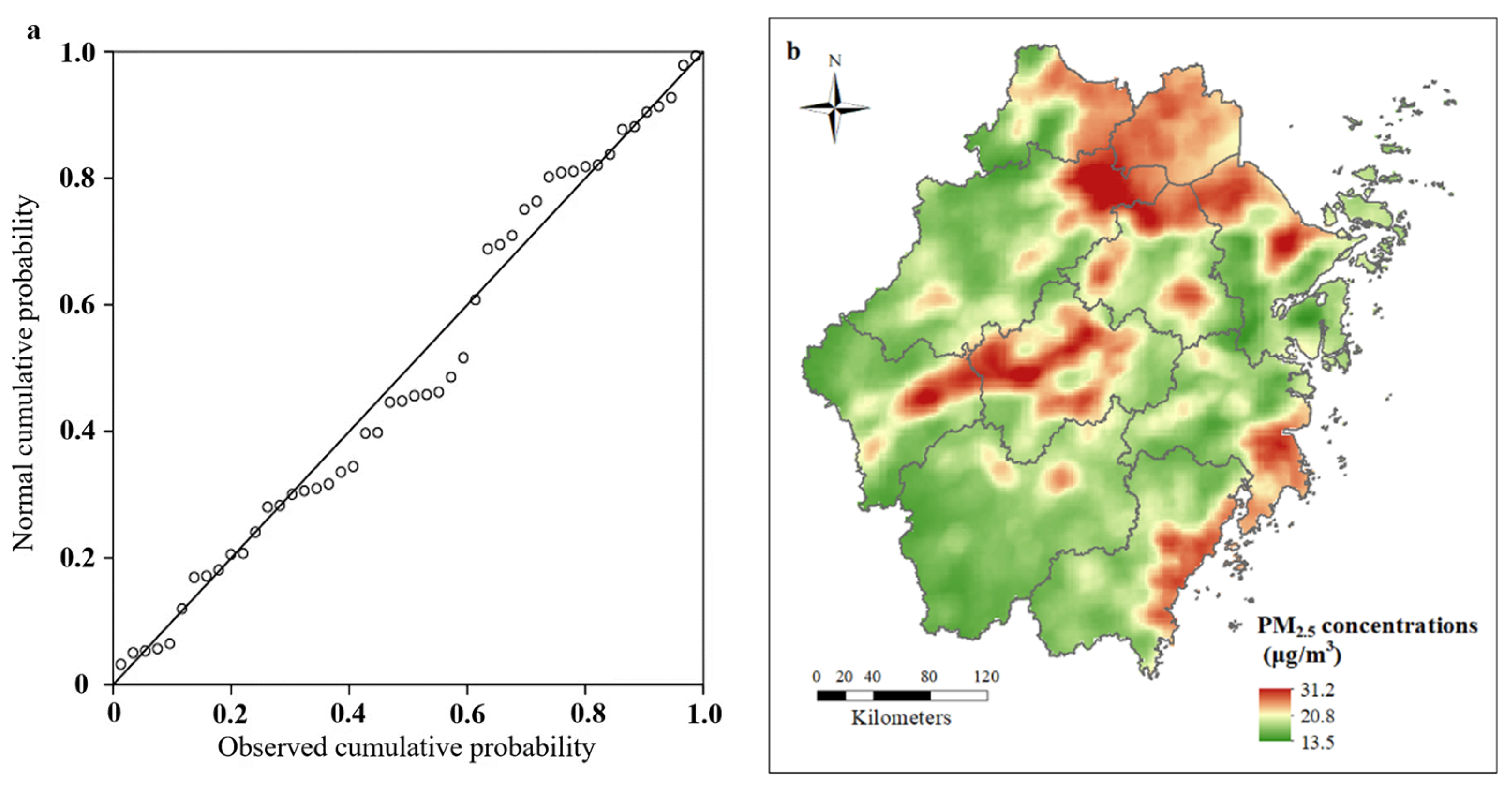
Figure 3a shows the probability–probability (P-P) plot of the standardized residuals. The scatter was distributed around the straight line y = x, indicating that the standardized residuals conform to a standard normal distribution, verifying that the regression hypothesis holds and that the data are reliable. The accuracy of the constructed model was then tested using the leave-one-out cross-validation method, and the RMSE was 2.56. Based on a 2 km × 2 km fishnet, Zhejiang Province was divided into a total of 26,329 grids, and each grid’s area of artificial surfaces within a buffer zone of 10 km radius, the area of forestland within a buffer zone of 10 km radius, and the annual average wind speed were extracted. The values of the explanatory variables were substituted into the obtained model and the gridded PM2.5 concentration values were calculated to simulate the spatial distribution of PM2.5 concentrations, as shown in Figure 3b.

3.2. Improved LUR Model Based on Geographically Weighted Regression

Since only a few variables were ultimately included in the regression equation, some variables that affect PM2.5 concentrations were ignored. In particular, there were differences between regions in socio-economic and natural environment, which may cause the relationship or structure between the explanatory variables and PM2.5 to change spatially. Therefore, this study considered the spatial heterogeneity and further analyzed the effect of the relevant factors in different regions based on the GWR method.
To avoid global multicollinearity between variables in the GWR, three factors, the area of artificial surfaces within a 10 km buffer zone radius, the area of forestland within a 10 km buffer zone radius, and the wind speed, were used as explanatory variables for the analysis. Figure 4 shows the coefficient of the three variables in the GWR. The results show that the area of artificial surfaces has a positive effect on the increase in PM2.5 concentration. This is attributed to the rapid expansion of artificial surfaces as urbanization progresses, gathering a large number of industrial activities, energy emissions, etc., which directly contributes to the increase in PM2.5 concentrations [11]. The coefficient of artificial surfaces gradually increases from northeast to southwest. This indicates that the area of artificial surfaces in southwest Zhejiang has a stronger positive effect on the increase in the PM2.5 concentration than that in northeast Zhejiang. The area of forestland has a negative effect on the increase in PM2.5 concentration. This is due to the dust-blocking effect of the vegetation leaves and absorption effect of the stem surfaces to weaken the PM2.5 concentrations [43]. The absolute value of the coefficient of forestland gradually increases from southwest to northeast. This indicates that forestland in northeast Zhejiang has a stronger negative effect on PM2.5 than in the southwest region. The coefficient of wind speed shows a trend that is higher in the east and lower in the west. As in the case of the annual mean wind speed, the effect on decreasing PM2.5 concentration may be enhanced as the wind speed increases.
The global adjusted R2 of the GWR model was 0.767. The local R2 of the samples ranged from a minimum of 0.53 to a maximum of 0.88, with an average of 0.65. The normality of the standardized residuals of the model was tested and the significance of the Shapiro–Wilk (S-W) test was 0.944, which is much greater than 0.05, indicating that it conforms to a normal distribution. The P-P plot of the standardized residuals is shown in Figure 5a. In addition, the standardized residuals should also show a random rather than a clustering distribution in terms of geographical distribution. The global Moran index (Moran I) was used for diagnosis and the results showed a global Moran index of −0.15 with a p-value of 0.23, with no significant clustering trend. The above analysis indicates that the model is reliable. Compared with the basic LUR model, the GWR-based improved LUR model has a higher simulation accuracy with a residual sum of squares of 148.18, an RMSE of 1.757, and an Akaike information criterion (AICc) of 214.73.
The simulation results of the spatial distribution of the GWR-based improved LUR model are shown in Figure 5b, which are generally consistent with the results of the multiple linear regression simulation. The PM2.5 pollution concentration areas are roughly the same, mainly in the urbanized areas of northern Zhejiang, central Zhejiang, and southeastern Zhejiang.

3.3. Improved LUR Model Based on Random Forest Regression

The improved LUR model based on random forest regression aims to use the screened factors as explanatory variables based on the results from the correlation analysis. Then, the random forest regression was applied for model construction. The training and validation sets were divided in a ratio of 8:2. The optimal parameters were determined using a random search cross-validation method. The number of decision trees in the final model was 600, and the maximum eigenvalue was 3.
The variables, in descending order of contribution to the model, are precipitation, cropland, grassland, forestland, wind speed, population, and artificial surfaces. Unlike the stepwise regression screening results, precipitation and cropland played a greater role in the random forest model.
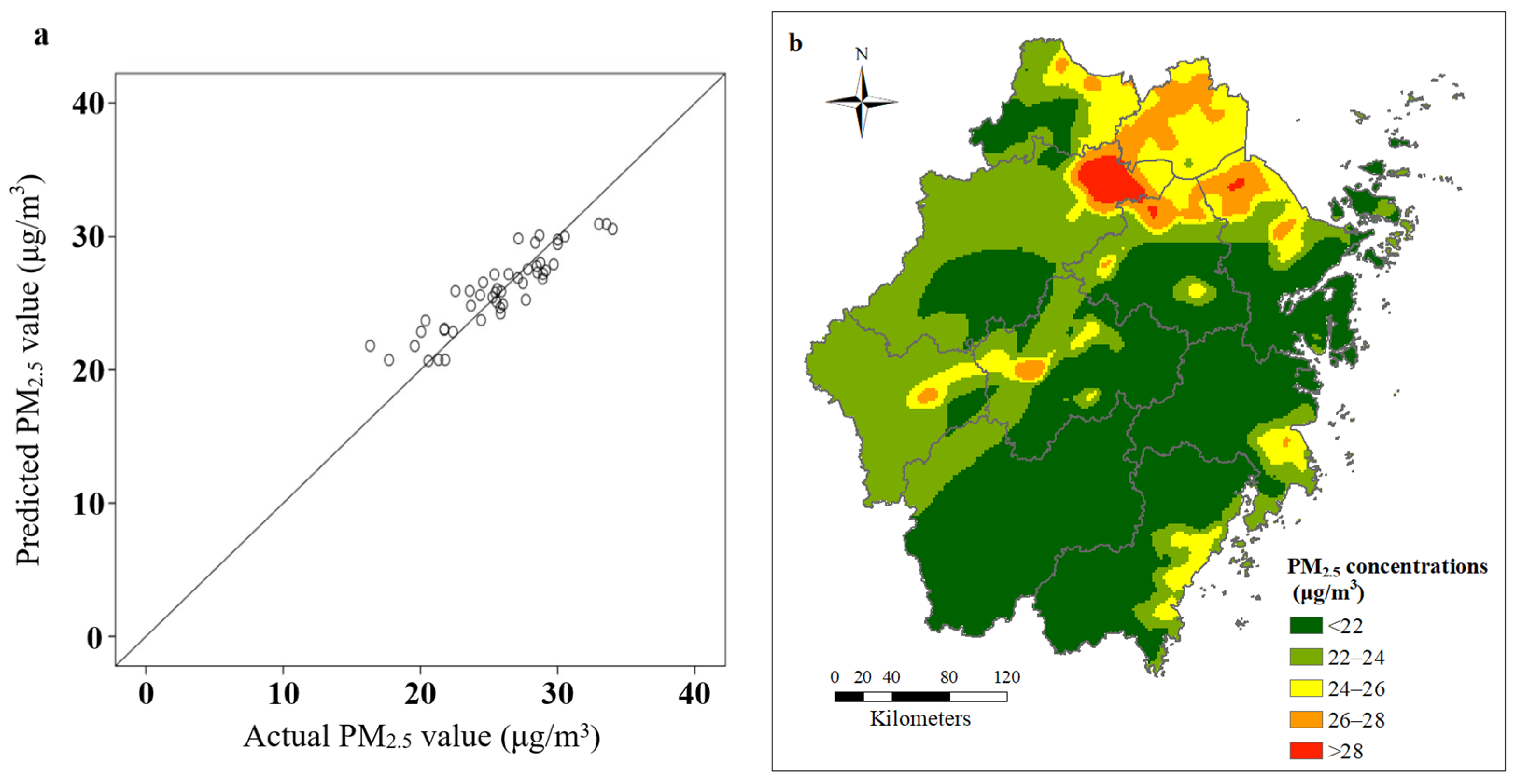
Figure 6a shows the linear fit of the model predictions to the actual values. The predicted values of the model largely matched the actual values, with the scatter concentrated around the diagonal line, indicating a good fit. The adjusted R2 for the training set of the model was 0.82, with an RMSE of 2.64 and a mean absolute error (MAE) of 1.34. The adjusted R2 for the validation set was 0.65, with an RMSE of 6.04 and a MAE of 1.90.
The simulation results of spatial distribution based on random forest regression are shown in Figure 6b, which are significantly different from those of multiple linear regression and GWR simulation, but the judgment of high pollution areas is roughly the same.

3.4. Model Comparisons

The evaluation of the different models on each indicator is shown in Table 3. To deepen the understanding of the different models, a comparative analysis of the regression models is provided, based on indicators such as MAE, RMSE, adjusted R2, and modified AICc.
It can be seen that the GWR-based improved LUR model performs better on all four indicators compared to multiple linear regression. The GWR-based improved LUR model shows less deviation between predicted and measured values, better accuracy of model fit, and higher precision. However, it is also noteworthy that the results of multiple stepwise linear regression identify the relevant factors which provide the best fit for GWR. The RF-based LUR model has a much higher adjusted coefficient of determination for the training set and a much smaller MAE, while also performing well in the validation set. However, the RMSE is relatively large, which could be attributed to the limited samples, making the fit results more accidental. It indicates that the accuracy of the model needs to be improved by introducing more samples or selecting more suitable explanatory variables to take advantage of the random forest’s ability to handle a large number of explanatory variables. Similar to previous studies with a small number of monitoring sites [44,45], here we achieved the spatial distribution of PM2.5 concentrations based on 49 monitoring sites, but the issue of distribution and the number of monitoring sites still needs to be addressed in the future. More monitoring sites could increase the precision of PM2.5 concentration estimation [46]. Furthermore, although an improved LUR model with acceptable accuracy was developed using GWR and RF, the accuracy of this model could be further improved by introducing more predictors under a spatially uniform distribution of monitoring stations.
The average PM2.5 concentrations obtained by different methods for each city in 2020 were compared and analyzed, and the results are shown in Table 4. The values in the three models were derived from the zonal statistics of the raster simulation results. The overall trend of PM2.5 spatial distribution in Zhejiang Province obtained by different methods is similar, but the average PM2.5 concentrations in prefecture-level cities obtained from different models are quite different. First, the average PM2.5 concentrations obtained based on the national control air quality monitoring sites are generally larger. This is because apart from the control points, the vast majority of stations are arranged within the urban area of the city. As analyzed in the previous section, urban areas are where PM2.5 pollution sources are concentrated, and land use patterns are not conducive to PM2.5 dispersion. Therefore, the average value based on monitoring stations mainly reflects the pollution situation in the urban area. However, the zonal statistics results obtained through the models reflect the city-wide pollution concentration.
Due to the different underlying logic and methodology, the results based on the regression model simulations differ significantly from those based on the monitoring sites; (the simulated average PM2.5 concentrations are relatively low), while the differences between the different regression models are relatively small. Geographically weighted regression simulations yielded the lowest mean PM2.5 concentrations for each city in the zonal statistics. It is also worth noting the relatively high estimate of pollution for Jiaxing at 26.35 μg/m³. Due to the inclusion of more explanatory variables and a different model structure, the random forest regression simulation results give different PM2.5 pollution emissions for each city compared to the other two regression models. The simulation results of the RF-based improved LUR show a small difference between the upper and lower limits.

4. Conclusions

We established a basic LUR model and improved LUR models based on geographically weighted regression and random forest methods to simulate the distribution of PM2.5 concentration. The basic LUR model was established based on the multiple stepwise linear regression method. The three elements of artificial surfaces, forest land, and wind speed were finally included as explanatory variables. The model was well fitted with an adjusted R2 of 0.645. The average RMSE of the leave-one-out cross-validation was 2.56. The results of the basic LUR model show that PM2.5 pollution was concentrated in the northern part of Zhejiang Province. The concentrations were also higher in regions such as the river valley plains in central Zhejiang and the coastal plains in southeastern Zhejiang. The explanatory variables of the GWR-based improved LUR model exhibited spatial heterogeneity. The adjusted R2 of the GWR-based improved LUR model reached 0.767, showing a better fit. In the RF-based improved LUR model, precipitation and cropland showed greater contribution than the factors of artificial surfaces, forest land, and wind speed. The adjusted R2 of the training model reaches 0.821, which is a significant improvement compared with the basic LUR model. The PM2.5 concentration simulation results of different models differ in some regions, but the distribution of high-pollution areas in three models are roughly the same, concentrated in northern Zhejiang, the river valley plains in central Zhejiang, and the coastal plains in southeastern Zhejiang. These findings indicate that more effective measures to reduce air pollutants need to be implemented.

Author Contributions

Conceptualization, S.Z.; data curation, C.Z.; formal analysis, C.Z. and X.W.; funding acquisition, S.Z.; methodology, S.Z., C.Z. and X.W.; supervision, S.Z.; validation, C.Z.; writing—original draft, S.Z., C.Z. and X.W.; writing—review and editing, S.Z. and X.W. All authors have read and agreed to the published version of the manuscript.

Funding

This research was funded by the National Natural Science Foundation of China (Grant No. 42007194); and the open fund by Jiangsu Key Laboratory of Atmospheric Environment Monitoring and Pollution Control (KHK1907).

Institutional Review Board Statement

Not applicable.

Informed Consent Statement

Not applicable.

Data Availability Statement

The data in the article are detailed in Section 2.1. All the data used are reflected in the article. If you need other relevant data, please contact the authors.

Acknowledgments

The authors are grateful to the China National Environmental Monitoring Centre (CNEMC, http://www.cnemc.cn/, accessed on 20 June 2022) for making PM2.5 data in Zhejiang, China for 2020 available. The authors are thankful to the OpenStreetMap (OSM, https://www.openstreetmap.org, accessed on 20 June 2022) for the road data in Zhejiang, China.

Conflicts of Interest

The authors declare no conflict of interest.

Appendix A

Table A1. Correlation coefficients between the area of each land type and PM2.5 concentration at different buffer radii. The missing value is attributed to insufficient data on the area of forestland within a buffer zone of 2 km.
Types2 km3 km5 km10 km
Area of cropland0.0530.0600.0410.308 *
Area of forestland-−0.389 **−0.483 **−0.485 **
Area of grassland−0.244 *−0.323 *−0.399 **−0.533 **
Area of water−0.180−0.177−0.1220.064
Area of artificial surfaces0.331 *0.375 **0.523 **0.545 **
** Correlation is significant at the 0.01 level (two-tailed); * correlation is significant at the 0.05 level (two-tailed).
Table A2. Correlation coefficients between geographical elements of emission sources and PM2.5 concentration at different buffer radii.
Types2 km3 km5 km10 km
Length of all roads0.345 **0.382 **0.477 **0.525 **
Number of factories−0.027−0.141−0.0700.140
Number of catering services0.1460.270 *0.400 **0.456 **
Number of car parks0.276 *0.336 **0.443 **0.470 **
Number of petrol stations0.268 *0.291 *0.472 **0.575 **
** Correlation is significant at the 0.01 level (two-tailed); * correlation is significant at the 0.05 level (two-tailed).
Table A3. Correlation coefficients between meteorology and PM2.5 concentration.
TypesCorrelation coefficients
Annual average wind speed−0.247 **
Annual precipitation0.492 **
Annual air temperature−0.121
Annual sea level pressure0.113
** Correlation is significant at the 0.01 level (two-tailed).
Table A4. Correlation coefficients between population and PM2.5 concentration at different buffer radii.
Types2 km3 km5 km10 km
Population0.2430.256 *0.376 **0.422 **
** Correlation is significant at the 0.01 level (two-tailed); * correlation is significant at the 0.05 level (two-tailed).

References

  1. Zhou, L.; Chen, X.; Tian, X. The impact of fine particulate matter (PM2.5) on China’s agricultural production from 2001 to 2010. J. Clean Prod. 2018, 178, 133–141. [Google Scholar] [CrossRef]
  2. Zheng, S.; Schlink, U.; Ho, K.F.; Singh, R.P.; Pozzer, A. Spatial distribution of PM2.5-related premature mortality in China. Geohealth 2021, 5, e2021GH000532. [Google Scholar] [CrossRef] [PubMed]
  3. Zheng, S.; Wu, X.; Lichtfouse, E.; Wang, J. High-resolution mapping of premature mortality induced by atmospheric particulate matter in China. Environ. Chem. Lett. 2022, 1–9. [Google Scholar] [CrossRef]
  4. Wang, Q.; Luo, K.; Fan, J.; Gao, X.; Cen, K. Spatial distribution and multiscale transport characteristics of PM2.5 in China. Aerosol Air Qual. Res. 2019, 19, 1993–2007. [Google Scholar] [CrossRef] [Green Version]
  5. Chang, X.; Wang, S.X.; Zhao, B.; Xing, J.; Liu, X.X.; Wei, L.; Song, Y.; Wu, W.J.; Cai, S.Y.; Zheng, H.T.; et al. Contributions of inter-city and regional transport to PM2.5 concentrations in the Beijing-Tianjin-Hebei region and its implications on regional joint air pollution control. Sci. Total Environ. 2019, 660, 1191–1200. [Google Scholar] [CrossRef]
  6. Chen, G.B.; Li, S.S.; Knibbs, L.D.; Hamm, N.A.S.; Cao, W.; Li, T.T.; Guo, J.P.; Ren, H.Y.; Abramson, M.J.; Guo, Y.M. A machine learning method to estimate PM2.5 concentrations across China with remote sensing, meteorological and land use information. Sci. Total Environ. 2018, 636, 52–60. [Google Scholar] [CrossRef]
  7. Juda-Rezler, K.; Reizer, M.; Maciejewska, K.; Blaszczak, B.; Klejnowski, K. Characterization of atmospheric PM2.5 sources at a Central European urban background site. Sci. Total Environ. 2020, 713, 136729. [Google Scholar] [CrossRef]
  8. Bae, C.; Kim, B.U.; Kim, H.C.; Yoo, C.; Kim, S. Long-range transport influence on key chemical components of PM2.5 in the Seoul metropolitan area, South Korea, during the years 2012-2016. Atmosphere 2020, 11, 48. [Google Scholar] [CrossRef] [Green Version]
  9. Zheng, S.; Zhou, X.Y.; Singh, R.P.; Wu, Y.Z.; Ye, Y.M.; Wu, C.F. The spatiotemporal distribution of air pollutants and their relationship with land-use Patterns in Hangzhou City, China. Atmosphere 2017, 8, 110. [Google Scholar] [CrossRef] [Green Version]
  10. Feng, H.; Zou, B.; Tang, Y. Scale- and region-dependence in Landscape-PM2.5 correlation: Implications for urban planning. Remote Sens. 2017, 9, 918. [Google Scholar] [CrossRef] [Green Version]
  11. Lu, D.B.; Mao, W.L.; Yang, D.Y.; Zhao, J.N.; Xu, J.H. Effects of land use and landscape pattern on PM2.5 in Yangtze River Delta, China. Atmos. Pollut. Res. 2018, 9, 705–713. [Google Scholar] [CrossRef]
  12. Wang, X.M.; Tian, G.H.; Yang, D.Y.; Zhang, W.X.; Lu, D.B.; Liu, Z.M. Responses of PM2.5 pollution to urbanization in China. Energ. Policy 2018, 123, 602–610. [Google Scholar] [CrossRef]
  13. Lu, D.B.; Mao, W.L.; Xiao, W.; Zhang, L. Non-linear response of PM2.5 pollution to land use change in China. Remote Sens. 2021, 13, 1612. [Google Scholar] [CrossRef]
  14. Shao, J.J.; Ge, J.F.; Feng, X.M.; Zhao, C.R. Study on the relationship between PM2.5 concentration and intensive land use in Hebei Province based on a spatial regression model. PLoS ONE 2020, 15, e0238547. [Google Scholar] [CrossRef] [PubMed]
  15. Goyal, P.; Gulia, S.; Goyal, S.K. Review of land use specific source contributions in PM2.5 concentration in urban areas in India. Air Qual. Atmos. Hlth. 2021, 14, 691–704. [Google Scholar] [CrossRef]
  16. Xu, W.Y.; Jin, X.B.; Liu, M.M.; Ma, Z.W.; Wang, Q.; Zhou, Y.K. Analysis of spatiotemporal variation of PM2.5 and its relationship to land use in China. Atmos. Pollut. Res. 2021, 12, 101151. [Google Scholar] [CrossRef]
  17. Briggs, D.J.; Collins, S.; Elliott, P.; Fischer, P.; Kingham, S.; Lebret, E.; Pryl, K.; van Reeuwijk, H.; Smallbone, K.; van der Veen, A. Mapping urban air pollution using GIS: A regression-based approach. Int. J. Geogr. Inf. Sci. 1997, 11, 699–718. [Google Scholar] [CrossRef] [Green Version]
  18. Abernethy, R.C.; Allen, R.W.; McKendry, I.G.; Brauer, M. A land use regression model for ultrafine particles in Vancouver, Canada. Environ. Sci. Technol. 2013, 47, 5217–5225. [Google Scholar] [CrossRef] [Green Version]
  19. Amini, H.; Schindler, C.; Hossein, V.; Yunesian, M.; Kunzli, N. Land use regression models for Alkylbenzenes in a middle eastern megacity: Tehran Study of Exposure Prediction for Environmental Health Research (Tehran SEPEHR). Environ. Sci. Technol. 2017, 51, 8481–8490. [Google Scholar] [CrossRef] [Green Version]
  20. Han, L.; Zhao, J.Y.; Gao, Y.J.; Gu, Z.L.; Xin, K.; Zhang, J.X. Spatial distribution characteristics of PM2.5 and PM10 in Xi’an City predicted by land use regression models. Sustain. Cities Soc. 2020, 61, 102329. [Google Scholar] [CrossRef]
  21. Wang, H.Z.; Yilihamu, Q.; Yuan, M.N.; Bai, H.T.; Xu, H.; Wu, J. Prediction models of soil heavy metal(loid)s concentration for agricultural land in Dongli: A comparison of regression and random forest. Ecol. Indic. 2020, 119, 106801. [Google Scholar] [CrossRef]
  22. Wu, J.S.; Li, J.C.; Peng, J.; Li, W.F.; Xu, G.; Dong, C.C. Applying land use regression model to estimate spatial variation of PM2.5 in Beijing, China. Environ. Sci. Pollut. R. 2015, 22, 7045–7061. [Google Scholar] [CrossRef] [PubMed]
  23. Yang, S.; Wu, H.T.; Chen, J.; Lin, X.T.; Lu, T. Optimization of PM2.5 estimation using landscape pattern information and land use regression model in Zhejiang, China. Atmosphere 2018, 9, 47. [Google Scholar] [CrossRef] [Green Version]
  24. Zhang, Y.; Cheng, H.G.; Huang, D.; Fu, C.B. High temporal resolution land use regression models with POI characteristics of the PM2.5 distribution in Beijing, China. Int. J. Env. Res. Pub. Heatlh 2021, 18, 6143. [Google Scholar] [CrossRef] [PubMed]
  25. Yang, D.Y.; Lu, D.B.; Xu, J.H.; Ye, C.; Zhao, J.A.; Tian, G.H.; Wang, X.G.; Zhu, N.N. Predicting spatio-temporal concentrations of PM2.5 using land use and meteorological data in Yangtze River Delta, China. Stoch. Env. Res. Risk A. 2018, 32, 2445–2456. [Google Scholar] [CrossRef]
  26. Zhang, Z.Y.; Wang, J.B.; Hart, J.E.; Laden, F.; Zhao, C.; Li, T.T.; Zheng, P.W.; Li, D.; Ye, Z.H.; Chen, K. National scale spatiotemporal land-use regression model for PM2.5, PM10 and NO2 concentration in China. Atmos. Environ. 2018, 192, 48–54. [Google Scholar] [CrossRef]
  27. Mo, Y.Z.; Booker, D.; Zhao, S.Z.; Tang, J.; Jiang, H.X.; Shen, J.; Chen, D.H.; Li, J.; Jones, K.C.; Zhang, G. The application of land use regression model to investigate spatiotemporal variations of PM2.5 in Guangzhou, China: Implications for the public health benefits of PM2.5 reduction. Sci. Total Environ. 2021, 778, 146305. [Google Scholar] [CrossRef]
  28. Beckerman, B.S.; Jerrett, M.; Serre, M.; Martin, R.V.; Lee, S.J.; van Donkelaar, A.; Ross, Z.; Su, J.; Burnett, R.T. A hybrid approach to estimating national scale spatiotemporal variability of PM2.5 in the contiguous United States. Environ. Sci. Technol. 2013, 47, 7233–7241. [Google Scholar] [CrossRef] [Green Version]
  29. Yazdi, M.D.; Kuang, Z.; Dimakopoulou, K.; Barratt, B.; Suel, E.; Amini, H.; Lyapustin, A.; Katsouyanni, K.; Schwartz, J. Predicting fine particulate matter (PM2.5) in the Greater London Area: An ensemble approach using machine learning methods. Remote Sens. 2020, 12, 914. [Google Scholar] [CrossRef] [Green Version]
  30. Wong, P.Y.; Lee, H.Y.; Chen, Y.C.; Zeng, Y.T.; Chern, Y.R.; Chen, N.T.; Lung, S.C.C.; Su, H.J.; Wu, C.D. Using a land use regression model with machine learning to estimate ground level PM2.5. Environ. Pollut. 2021, 277, 116846. [Google Scholar] [CrossRef]
  31. Liu, C.; Henderson, B.H.; Wang, D.F.; Yang, X.Y.; Peng, Z.R. A land use regression application into assessing spatial variation of intra-urban fine particulate matter (PM2.5) and nitrogen dioxide (NO2) concentrations in City of Shanghai, China. Sci. Total Environ. 2016, 565, 607–615. [Google Scholar] [CrossRef] [PubMed]
  32. Hu, L.J.; Liu, J.P.; He, Z.Y. Self-adaptive revised land use regression models for estimating PM2.5 concentrations in Beijing, China. Sustainability 2016, 8, 786. [Google Scholar] [CrossRef] [Green Version]
  33. Wang, X.F.; He, S.L.; Chen, S.C.; Zhang, Y.L.; Wang, A.H.; Luo, J.B.; Ye, X.L.; Mo, Z.; Wu, L.Z.; Xu, P.W.; et al. Spatiotemporal characteristics and health risk assessment of heavy metals in PM2.5 in Zhejiang Province. Int. J. Env. Res. Pub. Health 2018, 15, 583. [Google Scholar] [CrossRef] [Green Version]
  34. Wang, X.D.; Yang, Z.Y. Application of fuzzy optimization model based on entropy weight method in atmospheric quality evaluation: A case study of Zhejiang Province, China. Sustainability 2019, 11, 2143. [Google Scholar] [CrossRef] [Green Version]
  35. Chen, J.; Chen, J.; Liao, A. Remote Sensing Mapping of Global Land Cover; Science Press: Beijing, China, 2016. (In Chinese) [Google Scholar]
  36. Jun, C.; Ban, Y.F.; Li, S.N. Open access to Earth land-cover map. Nature 2014, 514, 434. [Google Scholar] [CrossRef] [Green Version]
  37. Bondarenko, M.; Kerr, D.; Sorichetta, A.; Tatem, A.J. Census/Projection-Disaggregated Gridded Population Datasets for 189 Countries in 2020 Using Built-Settlement Growth Model (BSGM) Outputs. WorldPop, University of Southampton, UK. 2002. Available online: https://doi.org/10.5258/SOTON/WP00684 (accessed on 20 June 2022). [CrossRef]
  38. Yang, X.F.; Zheng, Y.X.; Geng, G.N.; Liu, H.; Man, H.Y.; Lv, Z.F.; He, K.B.; de Hoogh, K. Development of PM2.5 and NO2 models in a LUR framework incorporating satellite remote sensing and air quality model data in Pearl River Delta region, China. Environ. Pollut. 2017, 226, 143–153. [Google Scholar] [CrossRef]
  39. Fotheringham, A.S.; Yue, H.; Li, Z. Examining the influences of air quality in China’s cities using multi-scale geographically weighted regression. Trans. GIS 2019, 23, 1444–1464. [Google Scholar] [CrossRef]
  40. Hu, X.F.; Belle, J.H.; Meng, X.; Wildani, A.; Waller, L.A.; Strickland, M.J.; Liu, Y. Estimating PM2.5 Concentrations in the Conterminous United States Using the Random Forest Approach. Environ. Sci. Technol. 2017, 51, 6936–6944. [Google Scholar] [CrossRef]
  41. Henderson, S.B.; Beckerman, B.; Jerrett, M.; Brauer, M. Application of land use regression to estimate long-term concentrations of traffic-related nitrogen oxides and fine particulate matter. Environ. Sci. Technol. 2007, 41, 2422–2428. [Google Scholar] [CrossRef]
  42. Xu, X.Y.; Ge, Y.H.; Wang, W.D.; Lei, X.N.; Kan, H.D.; Cai, J. Application of land use regression to map environmental noise in Shanghai, China. Environ. Int. 2022, 161, 107111. [Google Scholar] [CrossRef]
  43. Lu, D.B.; Xu, J.H.; Yue, W.Z.; Mao, W.L.; Yang, D.Y.; Wang, J.Z. Response of PM2.5 pollution to land use in China. J. Clean. Prod. 2020, 244, 118741. [Google Scholar] [CrossRef]
  44. Wang, J.W.; Cohan, D.S.; Xu, H. Spatiotemporal ozone pollution LUR models: Suitable statistical algorithms and time scales for a megacity scale. Atmos. Environ. 2020, 237, 117671. [Google Scholar] [CrossRef]
  45. Hystad, P.; Demers, P.A.; Johnson, K.C.; Brook, J.; van Donkelaar, A.; Lamsal, L.; Martin, R.; Brauer, M. Spatiotemporal air pollution exposure assessment for a Canadian population-based lung cancer case-control study. Environ. Health 2012, 11, 22. [Google Scholar] [CrossRef] [PubMed] [Green Version]
  46. Zou, B.; Luo, Y.Q.; Wan, N.; Zheng, Z.; Sternberg, T.; Liao, Y.L. Performance comparison of LUR and OK in PM2.5 concentration mapping: A multidimensional perspective. Sci. Rep. 2015, 5, 8698. [Google Scholar] [CrossRef] [Green Version]
Figure 1. Location of the study area and spatial distribution of monitoring sites and land use types.
Atmosphere 13 01273 g001
Figure 2. Steps of the random forest regression model.
Atmosphere 13 01273 g002
Figure 3. (a) Standardized residual probability–probability (P-P) plot. (b) Multiple linear regression simulation results.
Atmosphere 13 01273 g003
Figure 4. The coefficient of artificial surfaces (a), forestland (b), and wind speed (c) in the geographically weighted regression (GWR).
Atmosphere 13 01273 g004
Figure 5. (a) Standardized residual P-P plot. (b) Simulation results of the GWR-based improved land use regression (LUR) model.
Atmosphere 13 01273 g005
Figure 6. (a) The predicted and actual values of the random forest model. (b) Simulation results of the random forest-based improved LUR model.
Atmosphere 13 01273 g006
Table 1. Correlation analysis results.
TypesFactorsExplanatory VariablesPearson’s Correlation Coefficients
Land useArea of cropland within a 10 km buffer zone radius of the monitoring stationCL0.308 *
Area of forestland within a 10 km buffer zone radius of the monitoring stationFL−0.485 **
Area of grassland within a 10 km buffer zone radius of the monitoring stationGL−0.533 **
Area of artificial surfaces within a 10 km buffer zone radius of the monitoring stationAS0.545 **
Geographical elements of emission sourcesLength of all roads within a 10 km buffer zone radius of the monitoring stationAR0.525 **
Length of trunk roads within a 10 km buffer zone radius of the monitoring stationTR0.449 **
Length of primary roads within a 10 km buffer zone radius of the monitoring stationPR0.543 **
Length of secondary roads within a 10 km buffer zone radius of the monitoring stationSR0.414 **
Number of catering services within a 10 km buffer zone radius of the monitoring stationCS0.456 **
Number of car parks within a 10 km buffer zone radius of the monitoring stationCP0.470 **
Number of petrol stations within a 10 km buffer zone radius of the monitoring stationPS0.575 **
MeteorologyAnnual average wind speedWS−0.247 **
Annual precipitationPrec0.492 **
PopulationPopulation within a 10 km buffer zone radius of the monitoring stationPop0.422 **
** Correlation is significant at the 0.01 level (two-tailed); * correlation is significant at the 0.05 level (two-tailed).
Table 2. Multiple stepwise linear regression model parameters.
VariablesCoefficientTBetaVIFAd-R2RMSEp-Value
Intercept34.23486812.933 **--0.6452.460.000 **
AS0.0000563.759 **0.4161.619
FL−0.000072−3.851 **−0.4461.777
WS−0.424674−5.690 **−0.5251.126
** Correlation is significant at the 0.01 level (2-tailed); T: t-test statistic value; Beta: standardized coefficient; VIF: variance inflation factor; RMSE: root mean square error.
Table 3. Regression model evaluation.
MAERMSEAdjust R2AICc
Multiple linear regression1.952.460.645229.94
Geographically weighted regression1.391.760.767214.73
Random forest training set1.342.640.821-
Random forest validation set1.906.040.645-
MAE: mean absolute error; RMSE: root mean square error; AICc: Akaike information criterion.
Table 4. Each city’s average PM2.5 concentrations based on monitoring stations and regression model simulations.
Monitoring Sites (μg/m³)Multiple Linear Regression (μg/m³)Geographically Weighted Regression (μg/m³)Random Forest Regression (μg/m³)
Hangzhou28.8619.3217.6722.91
Ningbo22.9019.8519.4822.74
Wenzhou25.2319.2216.6621.90
Jiaxing27.8823.8726.3525.52
Huzhou25.9820.3319.0023.27
Shaoxing28.6020.9121.1122.43
Jinhua27.4621.4519.9421.83
Quzhou25.9618.7317.2923.07
Zhoushan16.7518.6418.4522.01
Taizhou24.5319.5118.4921.49
Lishui21.2317.2915.7221.17
Zhejiang Province25.0319.6018.4522.36
Publisher’s Note: MDPI stays neutral with regard to jurisdictional claims in published maps and institutional affiliations.

