Statistical Research on Seismo-Ionospheric Ion Density Enhancements Observed via DEMETER

Abstract

In this paper, in order to investigate the correlation between seismic activity and ionospheric density variation, nighttime ion density (Ni) data from IAP onboard the Detection of Electro-Magnetic Emissions Transmitted from Earthquake Regions (DEMETER) satellite from 2005 to 2010 are used to carry out statistical analysis. Only data with kp ≤ 3 are selected to avoid density perturbations due to magnetic activity. The aftershocks are also carefully removed. The earthquake-related data were further strictly screened, and the apparent position of anomalies were normalized using Dobrovolsky’s radius. Real and pseudorandom earthquakes are compared and analyzed. The statistical results show that the postseismic effect is obvious; the Ni enhancements are more focused 3–5 days, 9–10 days, and 13–14 days before the earthquake; as the magnitude of earthquake increases, the apparent range and intensity of the ion density enhancements is also increased; and for medium–strong earthquakes, the position of disturbance will exceed Dobrovolsky’s radius.

1. Introduction

The earthquake preparation phase has influence on different physical and chemical processes from the lithosphere to the atmosphere and ionosphere [1,2,3,4]. A large number of studies show that important anomalies in plasma parameters are observed before earthquakes. In recent decades, many papers and monographs have been published on the ionospheric plasma perturbations associated with seismic activity. Scientists have used different data processing methods to explore characteristics of the plasma anomalies before the earthquake, including data variation in distance, time, etc. [5,6,7,8,9].

The lithosphere–atmosphere–ionosphere coupling (LAIC) mechanism is widely used to explain the variation in the ionospheric parameters in relation to major seismic activity [1,2,4,10]. Different models based on LAIC have been proposed. The model based on the theory of p-holes (positive holes), which are produced by the stress along the fault, was suggested and was successfully tested in a laboratory [1]. Pulinets and Ouzounov [4] conclude that formation of large ion clusters changes the conductivity of the boundary layer of the atmosphere and the parameters of the global electric circuit over active tectonic faults. Variations in atmospheric electricity are the main source of ionospheric anomalies over seismically active areas. Kuo et al. [10] considered the role of the earth’s magnetic field and suggested a possible mechanism for the alteration of the ionosphere: an upward electric charge flux from the earthquake preparation area along the magnetic field line produces the corresponding plasma enhancement just above the epicentral region and its conjugate point. Under LAIC theory, case studies and statistical research from in-situ plasma parameters have been conducted.

Case studies have proved that there are obvious ionospheric plasma disturbances in the period of time before and after earthquakes, and these disturbances mainly appear in a certain range around the epicenter [11,12,13,14,15] and over the magnetic conjugate region of epicenter [16,17]. In addition, variation in plasma structures, such as EIA and plasma bubbles, are also observed and are probably related to earthquakes [6,16,18].

Statistical studies can provide common features of a lot of seismic events. He et al. [19] demonstrated that electron density increases close to epicenters both in the Northern and the Southern Hemisphere, but the position of the anomaly is slightly shifted to the north in the Northern Hemisphere and to the south in the Southern Hemisphere. Sarkar et al. [20] discussed that short-middle term precursors for most of the earthquakes occur in a time span of 3–5 days, while a post effect is observed for almost all the earthquakes up to a time span of 4 days. The registered electron density anomalies spread across an area of hundreds of kilometers in diameter. Statistical analyses have been performed using plasma density in the DEMETER dataset (6.5 years) and concluded that perturbations probably appear more southeast of the epicenter before earthquakes, and that there is an obvious trend which perturbations appear west of the conjugated point of an earthquake epicenter [17]. Liu et al. [21] found that more perturbations were seen in 1, 3, 5, 6, and 8 days before EQs and 1 day after EQs. In regard to spatial distribution, the anomalies before EQs were not just above the epicenters, but shifted equatorward by several degrees to almost twenty degrees.

Superposed epoch method analyses have been performed for the TEC anomalies associated with earthquakes (M > 6.0) during the 12-year period from May 1998–May 2010 by Kon et al. [22], and the statistical results indicate the significance of the positive TEC anomalies 1–5 days before earthquakes within 1000 km from the epicenter. Yan et al. [23] also used the superposed epoch method to perform statistical research on DEMETER data and found an anomalous increase in Ni related to earthquakes with M ≥ 5, while Ni fluctuations occur up to 200 km from the epicenters and mainly 5 days before earthquakes. On this basis, Zhu et al. [24] conducted a statistical study using CSES data and concluded that the significant variations of positive Ne and negative Te related to earthquakes mainly occurred ~1–7 days and ~13–15 days before the earthquakes, respectively, and within 200 km from the epicenters. Throughout the literature, most studies have limited the space–time range of anomalies to within a radius of 10° or 1500 km around the epicenter and 15 days before the earthquake. De Santis et al. [25] expanded the time and distance range and then carried out a statistical study using Swarm data. They found that some clear concentrations of electron density and magnetic anomalies are from more than two months to several days before the occurrence of an earthquake.

In view of the methods and conclusions from the above statistical research, the relationship between the location of anomalies and the epicenter is a very interesting phenomenon worth further discussion. In addition, the accurate selection of data related to an earthquake will affect the final statistical results. As such, exclusion of data affected by multiple earthquakes is required. Therefore, this study further investigates these issues. The purpose of this paper is to explore the time and spatial characteristics of plasma anomalies related to earthquakes using the improved method based on 6 years’ worth of DEMETER data. Section 2 and Section 3 describes the data and their processing methods, Section 4 and Section 5 present the results and discussions separately, and the conclusions are summarized in Section 6.

2. Data and Earthquakes

The ion density (Ni) from IAP onboard DEMETER from 2005 to 2010 are used in this paper. The detail of the IAP experiment can be found in Berthelier et al. [26]. As the density variation is strongly dominated by the sun during daytime, only nighttime data are selected. We also removed data during kp > 3 to avoid density perturbations due to magnetic activity.

The considered earthquake database includes 20,547 earthquakes with M ≥ 4.8 occurring from 2005 to 2010 (U.S. Geological Survey: http://www.usgs.gov, accessed on 1 May 2021). The aftershocks in the list of earthquakes are carefully removed by characterizing the occurrence time and its associated area of main shock. That is, for a given earthquake in the list, any other earthquake that occurred inside the area of 2° × 2° centered on the epicenter and within 15 days after its occurrence time is systematically removed from the list (see the detail in Yan et al. [23]). After this, 10,320 earthquakes (EQs) are remaining in the list. The global distribution of these EQs is shown in Figure 1a.

To check the reliability of the results from real earthquakes, a list of pseudorandom EQs is generated to be analyzed by the same statistical analysis. The statistical results will be compared with those from the list of real earthquakes. Pseudorandom earthquakes were generated as follows: the longitudes of the 10,320 real earthquakes epicenter have been shifted by 10° to the west, and the occurring time has been set to advance by a month. This was conducted to try to keep the same ionospheric conditions, because most of the earthquakes are concentrated around the equator, and the one-month shift of time was also to stay at the same season [27]. The global distribution of pseudorandom earthquakes is shown in Figure 1b.

3. Method

In this study, the basic data processing progress is the same as that of Yan et al. [23]; however, some adjustments and improvements were made, i.e., the selection of data is more strictly limited, and the apparent position of anomalies is normalized using Dobrovolsky’s radius. Details are given as follows.

Firstly, we built background maps with a cell of 2° (lat) × 4° (lon) according to the sun cycle and the seasons. We classified the Ni background maps according to the monthly global distribution characteristics and intensity changes of Ni. In most cases, the data during May–June–July–August are combined into one background map, data in November–December and January–February of the next year are merged into another background map, and data from March–April and September–October are merged in another background map. As data for 2004 and 2011 are not available, the data from January–February 2005 and November–December 2010 are each merged into their background map separately. In total, for the period 2005–2010, 19 background maps have been built.

Secondly, the density variations associated with seismic activity were exacted by comparing the data related to earthquakes with those of the background maps. The adjustment and improvements of methods adopted are in this section.

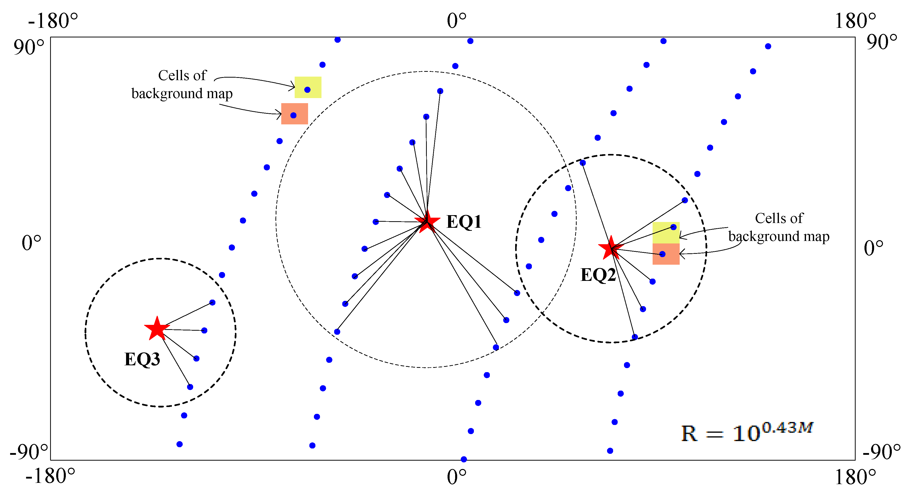
It is generally accepted that the radius of the effective precursor manifestation zone is given by Dobrovolsky’s formula, R = 10^0.43M. In the formula, the radius of the earthquake preparation zone is in kilometers and M is the earthquake’s magnitude [28]. We normalized the distance of apparent anomalies according to Dobrovolsky’s formula. For each earthquake, the relevant data were associated with Dobrovolsky’s radius R corresponding to the magnitude of this earthquake, instead of selecting the same distance range for all magnitude earthquakes. At the same time, we are still more interested in anomalies that take place in the short term (within two weeks). Therefore, the time interval of interest was corrected to be from 15 days before the occurrence time of earthquakes and until 5 days after.

In addition, to avoid the possibility that the used data may be affected or disturbed by multiple earthquakes, only data related to one earthquake were acquired. In order to solve this problem, in the first step all the data related to the earthquakes are labeled using ‘mark’, i.e., for each earthquake, the data during the period from 15 days before to 5 days after the earthquake and within Dobrovolsky’s radius R were selected and labeled. If this was affected by one earthquake, its mark was 1; If affected by two earthquakes, its mark was 2, etc. Then, all earthquakes and all data were labeled. Finally, a column of ‘mark’ was added to the data file to identify that the data point is affected by the number of earthquakes.

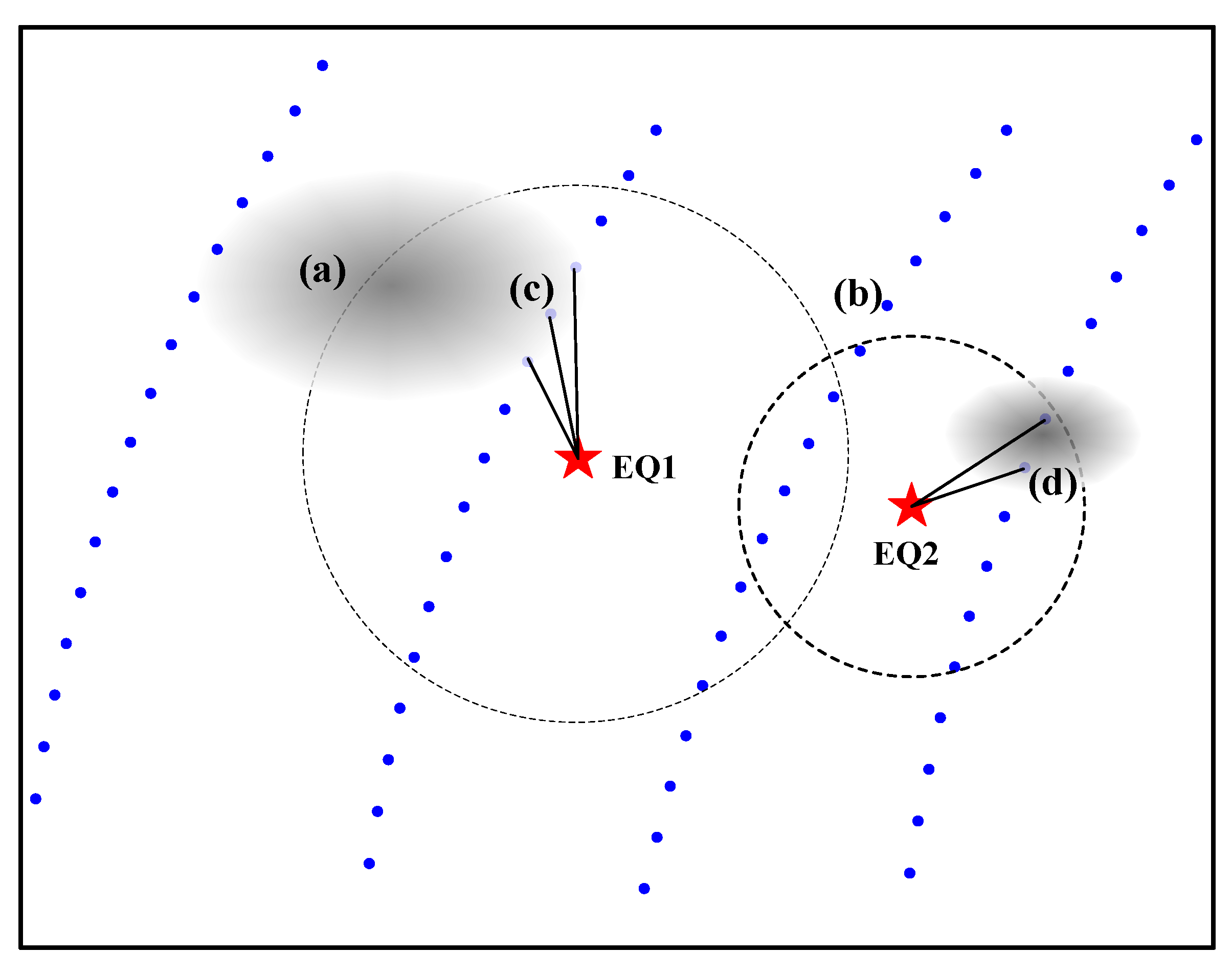
In order to explore whether the plasma anomaly in the ionosphere affected by the earthquake will be outside Dobrovolsky’s radius R, data within three times Dobrovolsky’s radius R were selected to perform statistical research. The specific data selection method was as follows: For each earthquake, the data with mark = 1 from 15 days before to 5 days after the earthquake and within Dobrovolsky’s radius R were obtained as the relevant data of the earthquake, which demonstrates that the selected data are only affected by this earthquake, shown in Figure 2. In Figure 2, the data points on the orbit (blue dots), earthquake epicenters (red star), and the areas of Dobrovolsky’s radius R around the epicenters (dashed circles) are shown. Data points that are only used for one earthquake (with mark = 1) is connected to the epicenter by black lines. While during the range from R to 3R for each earthquake, the data with mark = 0 during the period between 15 days before and 5 days after the earthquake are selected, which shows that, in theory, these data have not been affected by any earthquake.

Following that, the density variations of each datapoint for every earthquake is exacted [23]. Each datapoint is normalized considering the average and the standard deviation values in the corresponding cell of the background map. Then for each earthquake j, the new calculated quantity (D_i)_j is given by

$${(D_i(\Delta R,\Delta t))}_j=\frac{{(N_i(\Delta R,\Delta t))}_j-{\overline{X}}_j}{\sigma j}$$

(D_i)_j is a function of data location within the normalized Dobrovolsky’s radius (ΔR) of the considered earthquake and function of the time difference (Δt) between the measurement time of the data and the occurrence time of the earthquake j. ${\overline{X}}_j$ is the average value in the corresponding cell of the background map, and ${\sigma }_j$ is the deviation value.

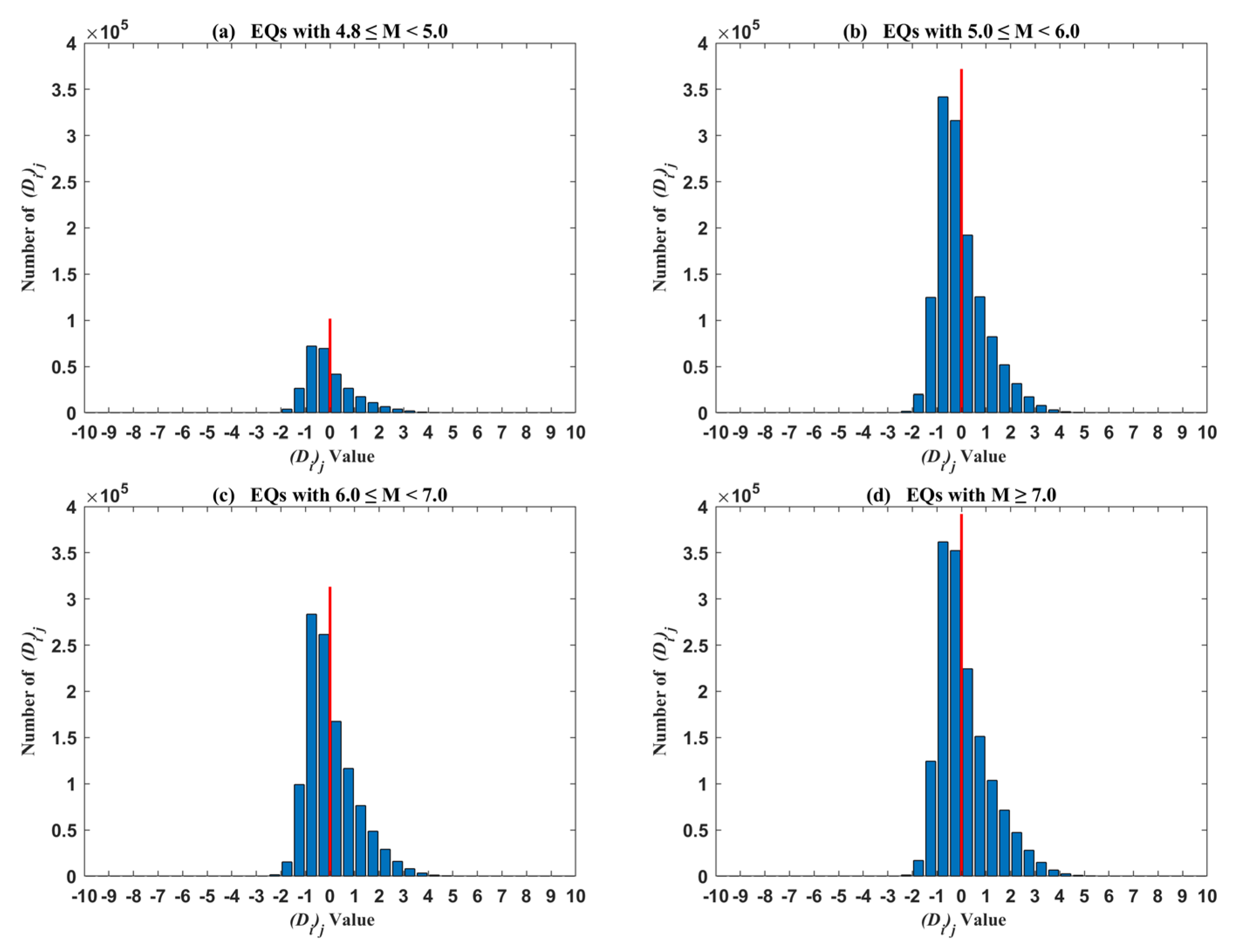
The histogram of the (D_i)_j values obtained from earthquakes with different magnitude is presented in Figure 3. For the four subpanels from earthquakes with different magnitudes in Figure 3, the distribution of negative (D_i)_j is roughly Gaussian, whereas the distribution of positive one is obviously not Gaussian. As discussed by previous research, if earthquakes would have no effects on the ionospheric ion density, then the statistics of Ni should be similar to the statistics of the ion density measurements used to build the background maps and, in such a case, the (D_i)_j distribution should be Gaussian-like [23]. Therefore, non-Gaussian-like positive (D_i)_j is probably affected by other factors, such as an earthquake. In addition, regarding some LAIC models an anomalous statistical increase in the ionospheric ion density above earthquakes is favored at the altitude of DEMETER [4,10,23]. Therefore, the positive (D_i)_j is of interest for our study. It should be noted that the amount of data in Figure 3a is obviously less than others because the Dobrovolsky’s radius R is small for earthquakes M < 5.

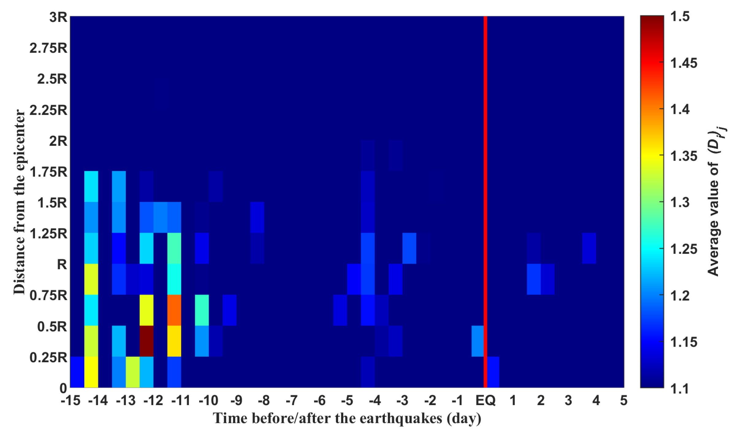
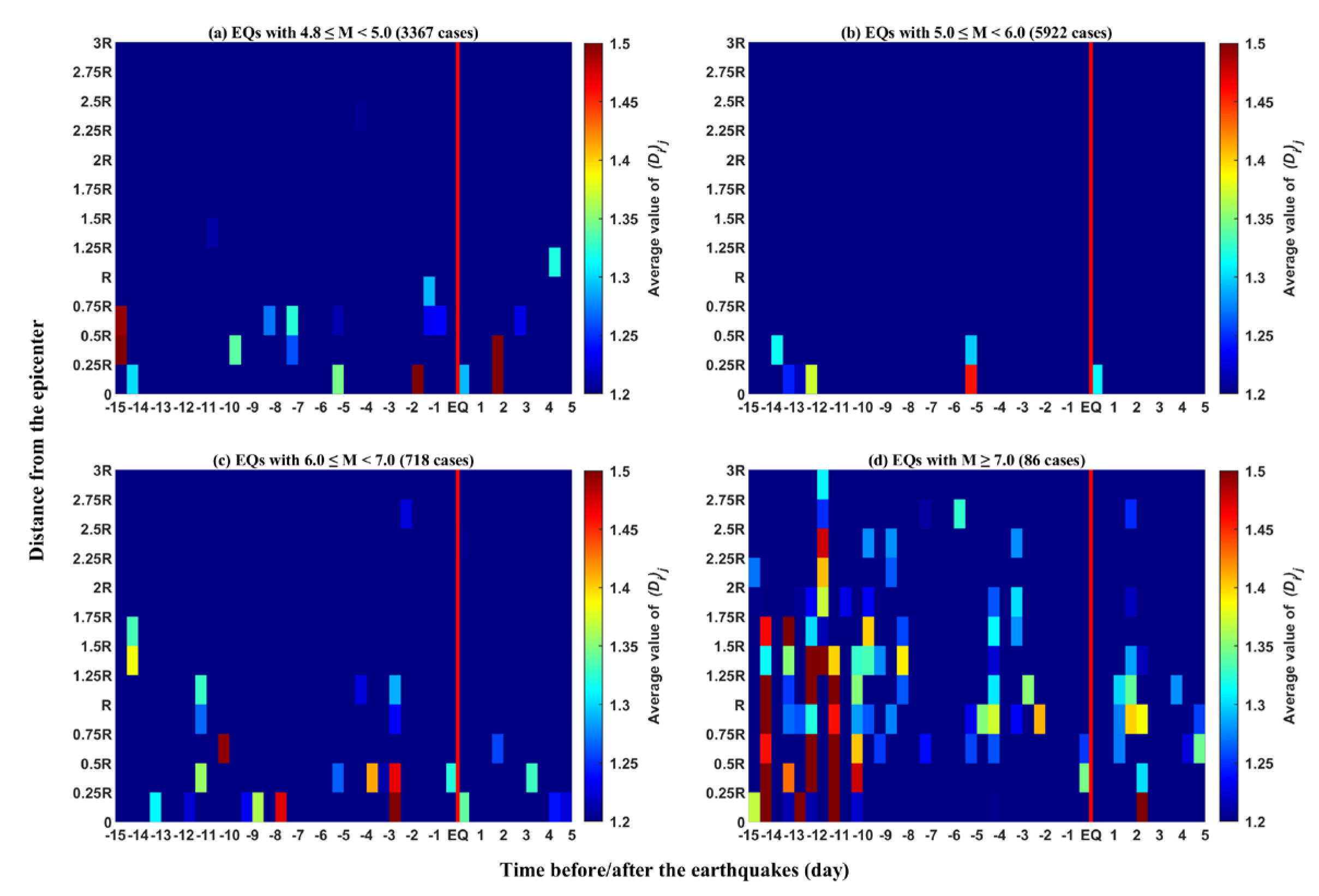
Finally, the superposed epoch method is used to present the final statistical results. A grid is considered where the horizontal (X) axis is related to time and the vertical (Y) axis is related to the distance. The X axis is from 15 days before to 5 days after the earthquake, with a resolution of 12 h. The Y axis is the normalized Dobrovolsky’s radius R, from 0 to 3R with a resolution of 0.25R. Therefore, the area of interest was taken as a disk with a radius of 3R centered on the epicenter of the earthquakes, and each ion density variation both inside the time interval and space area associated with an earthquake is considered. All earthquakes are assumed to occur at the time equal to 0 and at the same location (distance = 0). For each earthquake, the data are cumulated in appropriate cells with a dimension of 0.25R × 12 h. An average value of all positive (D_i)_j values in each cell is calculated and shown in figures according to the color scale.

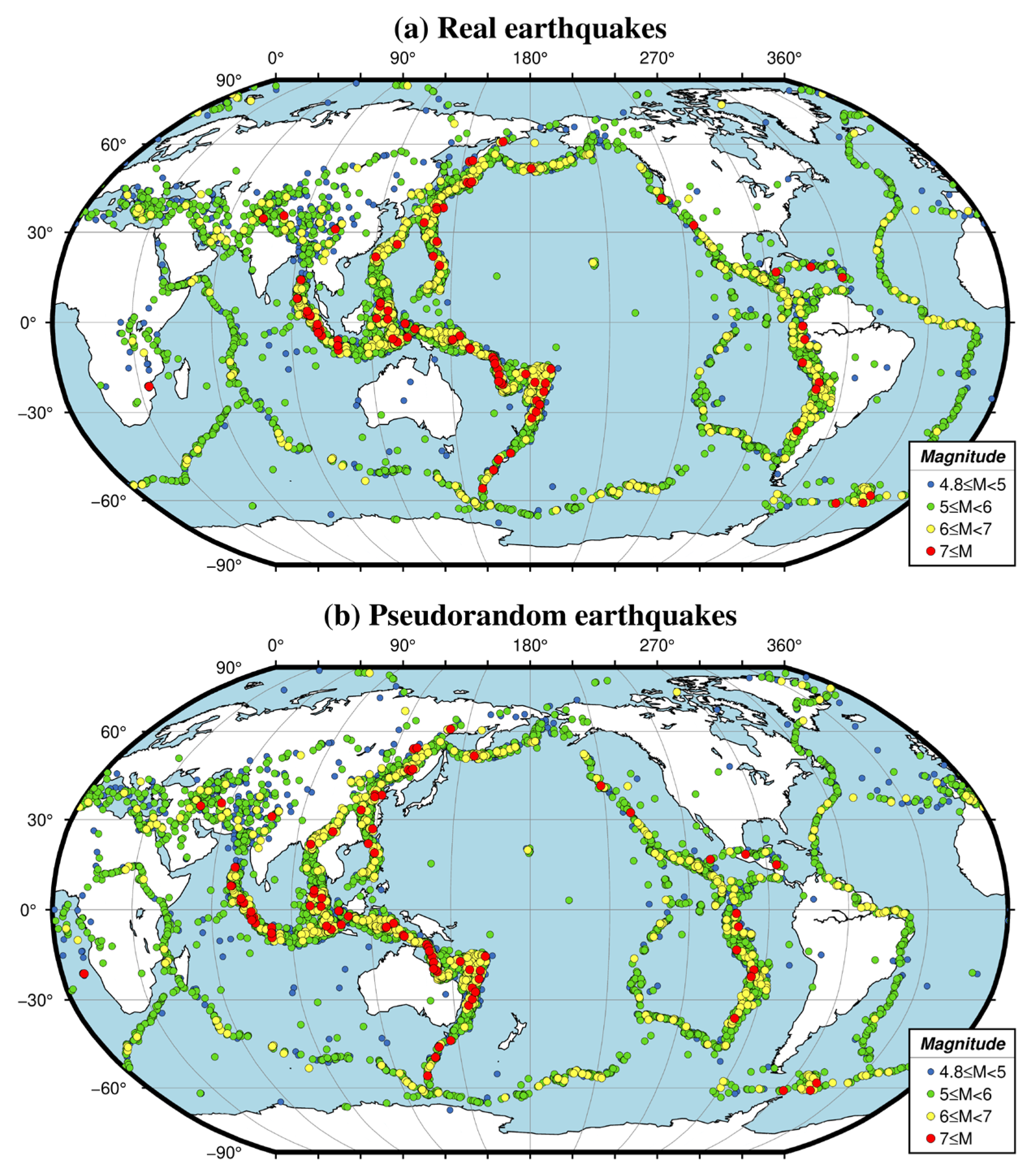
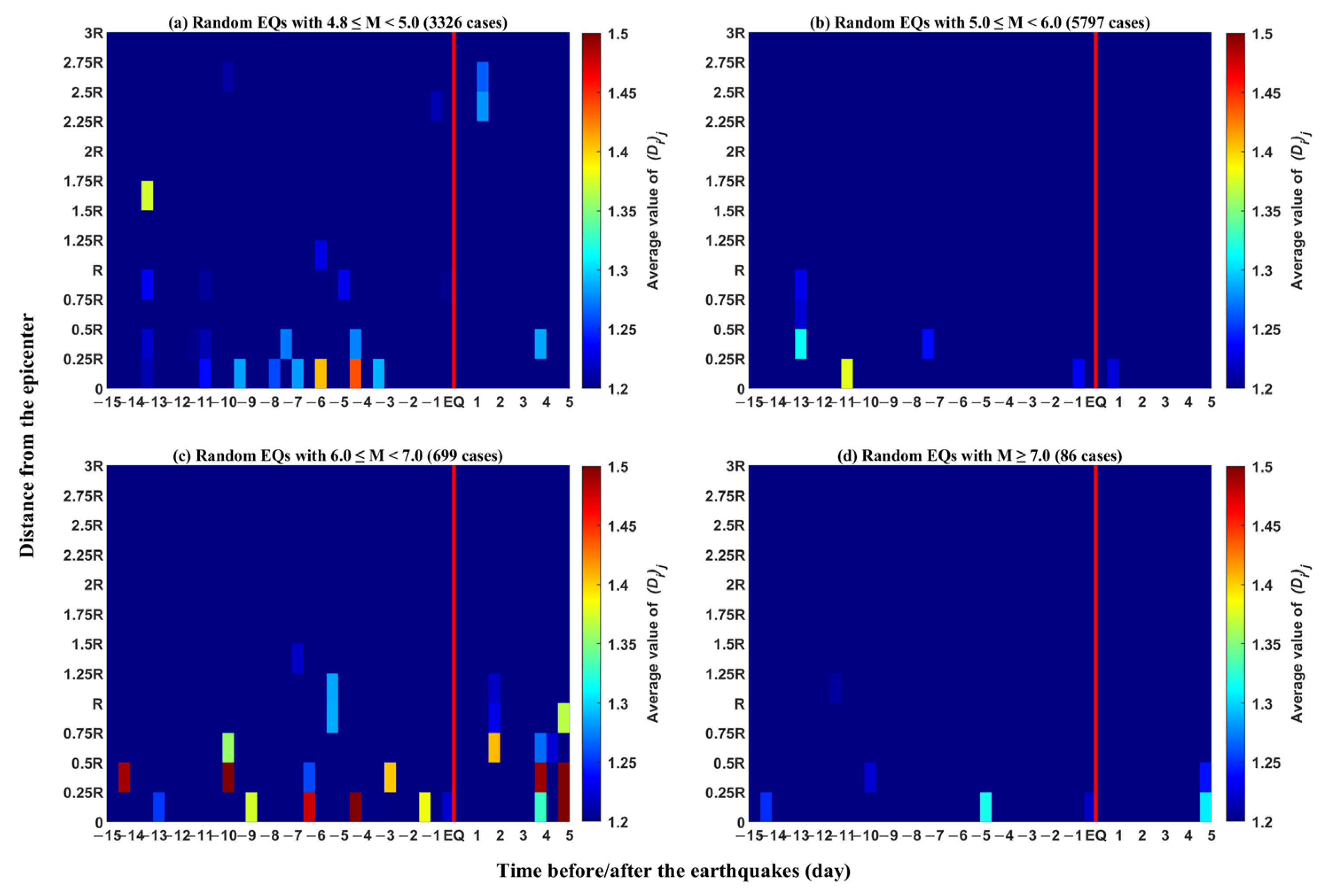
In order to compare the characteristics of seismic-related and random events, we repeat the above method for the random earthquake lists and also analyze the results. It is important to note here that data during the period from 15 days before and 5 days after the earthquake and within Dobrovolsky’s radius R are labeled using the random earthquakes list, so that the regularity of data associated with real earthquakes could be completely broken.

4. Results

4.1. The Results of Real EQs

Figure 4 represents the final statistical results from 10,093 earthquakes with M ≥ 4.8. It is noted that due to strict data selection, there may be earthquakes for which there are no data available and the final number of earthquakes used for statistical analysis will be smaller than the number of earthquakes in the main earthquake list. In Figure 4, more perturbations are observed from 10 days to 15 days before the EQ occurrence time. At the same time, 3–5 days before the earthquake was another period of significant disturbance. In addition, the postseismic effect is obvious. The apparent position of disturbance can extend to 1.75R.

Then, we separated the EQs into different sets and the results of the statistical analysis are shown in Figure 5, including EQs with M ≥ 4.8 and M < 5 (Figure 5a), EQs with M ≥ 5 and M < 6 (Figure 5b), EQs with M ≥ 6 and M < 7 (Figure 5c), and EQs with M ≥ 7 (Figure 5d). It can be found that, compared with the statistical results of all earthquake magnitudes together in Figure 4, the statistical results of earthquakes with different magnitude classifications have better regularity. Firstly, the postseismic effect in Figure 5a–c is obvious. This isa very important phenomenon that can be used to prove that signals related to earthquake can propagate to the ionosphere. Secondly, with an increase in magnitude, the temporal and spatial range of disturbance increases. For earthquakes with M < 6, the disturbance mainly occurs within the range of R, and for earthquakes with M ≥ 6, there are abnormal phenomenon that appear outside the range of R. Thirdly, as the magnitude increases, the disturbance becomes more intense.

Comparing Figure 4 and Figure 5d, it can be seen that the two figures have similar anomaly distribution characteristics. We infer that the abnormal phenomena 10–15 days before the earthquake in Figure 4 are mainly caused by earthquakes with M ≥ 7, rather than ones with M < 7. Therefore, compared with earthquakes with M < 7, the abnormal variations in plasma caused by earthquakes with M ≥ 7 are larger in both intensity and space–time range. In particular, the distance range has far exceeded the range of R radius. The variation can be physically understandable (shown in Figure 5).

4.2. The Results of Pseudorandom EQs

To confirm if the above statistical results of disturbance are related to earthquakes, we also studied the results of the pseudorandom earthquakes, as shown in Figure 6.

Compared with ones in Figure 5, obvious differences are observed in Figure 6: (1) there is no postseismic effect observed in all four panels; (2) The occurrence time of the disturbance before the earthquake is relatively scattered; (3) The intensity of the disturbance and the range of its occurrence do not change with magnitude. Especially for the results of earthquakes with M ≥ 7 in Figure 6d, the disturbance cannot even be observed. Compared to earthquakes with smaller magnitudes, it is obviously illogical for earthquakes with larger magnitudes to bring such weaker changes in plasma anomalies.

5. Discussion

The statistical results (Figure 5) are consistent with the conclusions of previous research. Especially for earthquakes set with M ≥ 5 and M < 6 (Figure 5b), the anomaly characteristics of spatial/temporal distribution and intensity shows more in line with expectations. The postseismic ionospheric disturbances have been demonstrated by many publications [20,23,25]; the spatio-temporal range variation of anomalies with different earthquake magnitudes have also been confirmed by the literature [11,12,13,14,15]. For example, Sarkar et al. [20] reported that for earthquakes with a moderate magnitude, the electron density anomalies occurred within 5 days before and after the earthquakes; however, for the great Sumatra earthquake of 28 March 2005, its lead time was around 14 days.

The newly obtained results in this paper show that the occurrence range of seismic ionospheric anomalies depend on the magnitude, and for medium–strong earthquakes, the occurrence range of anomalies will exceed Dobrovolsky’s radius R, as shown in Figure 5c,d. Many previous earthquake case studies have also confirmed these results, such as findings that the disturbance does not occur directly above the earthquake epicenter but is shifted towards the equatorial direction, and may occur in the magnetic conjugate region [17,21], or cause an increase in EIA [6]. Oyama et al. [9,13] concluded that the disturbance region extends to roughly 70° both east and west in longitude and about 20° to north and west from the epicenter. Theoretical simulations also support this expansion of range. According to the LAIC, it is believed that the earth surface electric field caused by earthquakes will deviate to the equatorial direction when it reaches the ionosphere along the magnetic field lines of the geomagnetic field [16]. Ryu et al. [18] concluded that the EIA was enhanced in the west of the epicenter and reduced in the east of the epicenter, which fits the ‘increased conductivity’ model. In this paper, for the earthquakes with M ≥ 6, the anomaly range tends to exceed the radius R of the earthquake preparation zone, especially for earthquakes with M ≥ 7, and there are obvious anomalies 12 days before the earthquake at approximately 2.5R from the epicenter. According to the earthquake preparation radius [28], when the earthquake with M = 7.5, its R will be approximately 1678 km, that is around 15°, its magnetic conjugate region may be located at 2.5R distance. These seem to be reasonable phenomena.

However, there are also unreasonable phenomena observed from the statistical results by different magnitude sets, such as the anomalies from the earthquakes with M ≥ 4.8 and M < 5 (Figure 5a) show greater variation and wider range than those from earthquakes with M ≥ 5.0 and M < 6 (Figure 5b). This is probably related to the amount of data used for statistical analysis and the number of earthquake cases (see the amount of data in Figure 3), as the amount of data used for statistics affects the final statistical result to a certain extent [29]. According to the location of each earthquake (ocean, land, or island), the underground electrical structure in the epicenter, and the different environment during the process of abnormal signal propagation from the lithosphere to the ionosphere, it is likely that the time of the anomalies before the earthquake and their location relative to the epicenter are uncertain. However, the DEMETER satellite cannot observe the same location for a long time, therefore, the anomaly data observed by the satellite are random relative to the earthquake. In this case, the more earthquake cases there are, the less the random the statistical results may be. Sufficient earthquakes and sufficient data superimposed in statistical studies will eliminate randomness and ensure that the results are more objective.

At the same time, we believe that the limitation of single satellite observation is also a main reason for this. A single satellite is always moving, rather than performing long-term tracking observation at a fixed position. Under the circumstances, as shown in Figure 7, when an anomaly appears, there may not be satellite passing by (such as the state of a), or when the satellite passes by, there is no apparent anomaly (such as the state of b). It is also possible that for the strong and large anomaly caused by earthquakes with a large magnitude, the satellite only passed the edge of the anomaly and measured weak variation, such as the state of (c) in Figure 7, while for the weak and small anomaly by earthquakes with small magnitude, the satellite passed right through the center of the anomaly and measured the strongest anomaly, such as the state of (d) in Figure 7. This leads to abnormal phenomena before the earthquake is observed whereby the satellite cannot fully correspond to the magnitude one by one.

The statistical results of random earthquakes can prove that the statistical results of real earthquakes are reasonable and reliable from another point of view, as shown in Figure 6. It can be seen that there is no postseismic phenomenon at all. In addition, with an increase in magnitude, the intensity and range do not regularly change. Especially for the statistics of earthquakes with M ≥ 7 in Figure 6d, there is barely any disturbance observed, which is obviously unreasonable. Meanwhile, because the same amount of data and earthquake cases are used in Figure 5 and Figure 6, it can also be explained that the abnormal phenomenon in Figure 5 is not caused by the difference in the amount of data used for the statistics. When we selected the data related to the random earthquake, the regularity of the data related to the real earthquake may be scrambled and the time and location of the abnormal phenomenon will not be concentrated. As a result, the statistical anomalies of random earthquakes (Figure 6) are weaker than those of real earthquakes (Figure 5).

In this study, to let the distance of occurrence anomalies have the same significance for earthquakes with all magnitude, Doborvolsky’s radius R was used to normalize the range of the occurrence of anomalies. At the same time, it was not limited to the range of R, but also extended to the distance of 3R. Dobrovolsky’s 3R varies greatly across earthquakes with different magnitudes, which will lead to differences in the amount of data obtained. Therefore, we classified earthquakes according to magnitudes carefully and more effectively obtained the distance characteristics for the abnormal seismic phenomenon. Comparing the results in this study to the results of Yan et al. [23], we can see that the position of anomalies in the two results is different. According to Dobrovolsky’s radius, for earthquakes with M = 5, Dobrovolsky’s radius R is around 141 km, while for earthquakes with M = 7, R is around 1023 km. The anomaly appeared mainly inside 600 km in the results from Yan et al. [23]. In this case, for earthquakes with a small magnitude, more abnormal data may be available closer to the epicenter, while for earthquakes with a large magnitude, some abnormal data may be missing in the far range. However, regardless of earthquake magnitude, anomalies within 600 km are more concentrated, so the results in Yan et al. [23] more effectively show the time characteristics of the anomaly.

6. Conclusions

In this paper, we performed statistical research on seismo-ionospheric ion density enhancements observed via DEMETER using the superposed epoch method. A strict screening of the earthquake-related data was carried out, and the locations of anomalies were normalized using Dobrovolsky’s radius according to the different magnitudes. In addition, real and pseudorandom earthquakes were compared and analyzed. The major findings are summarized as follows:

(1)

The postseismic ionospheric disturbances is very obvious;

(2)

With the magnitude of the earthquake increasing, the apparent range and intensity of anomaly is also increased;

(3)

The anomaly was focused on 3–5 days, 9–10 days, and 13–14 days before the earthquake;

(4)

For medium–strong earthquakes, the occurrence range of anomalies will exceed Dobrovolsky’s radius R.

The statistics results from pseudorandom earthquakes have no law, which confirms the regularity of earthquake related anomalies. The observed perturbations are real but can only be statistically evidenced. The radius of the earthquake preparation zone given by Dobrovolsky is an empirical formula, whether the radius is fully applicable to the study of seismo-ionospheric anomalies, more seismic parameters (such as depth, location, focal mechanism, etc.) need to be considered and more in-depth research should be carried out. Furthermore, in order to more effectively capture more real and objective abnormal information, simultaneous observation by multiple satellites may be more necessary.

References

1. Freund, F. Pre-earthquake signals: Underlying physical processes. J. Asian Earth Sci. 2011, 41, 383–400. [Google Scholar] [CrossRef]
2. Hayakawa, M.; Izutsu, J.; Schekotov, A.; Yang, S.-S.; Solovieva, M.; Budilova, E. Lithosphere–Atmosphere–Ionosphere Coupling Effects Based on Multiparameter Precursor Observations for February–March 2021 Earthquakes (M~7) in the Offshore of Tohoku Area of Japan. Geosciences 2021, 11, 481. [Google Scholar] [CrossRef]
3. Ouzounov, D.; Pulinets, S.; Romanov, A.; Romanov, A.; Tsybulya, K.; Davidenko, D.; Kafatos, M.; Taylor, P. Atmosphere-ionosphere response to the M9 Tohoku earthquake revealed by multi-instrument space-borne and ground observations: Preliminary results. Earthq. Sci. 2011, 24, 557–564. [Google Scholar] [CrossRef]
4. Pulinets, S.; Ouzounov, D. Lithosphere–Atmosphere–Ionosphere Coupling (LAIC) model—An unified concept for earthquake precursors validation. J. Asian Earth Sci. 2011, 41, 371–382. [Google Scholar] [CrossRef]
5. Ghamry, E.; Mohamed, E.K.; Abdalzaher, M.S.; Elwekeil, M.; Marchetti, D.; De Santis, A.; Hegy, M.; Yoshikawa, A.; Fathy, A. Integrating Pre-Earthquake Signatures From Different Precursor Tools. IEEE Access 2021, 9, 33268–33283. [Google Scholar] [CrossRef]
6. Gurram, P.; Kakad, B.; Ravi Kumar, M.; Bhattacharyya, A. Earthquake/Tsunami-Linked Imprints in the Equatorial F Region Zonal Plasma Drifts and Spatial Structures of Plasma Bubbles. J. Geophys. Res. Space Phys. 2019, 124, 504–520. [Google Scholar] [CrossRef]
7. Hayakawa, M.; Molchanov, O.A.; Kodama, T.; Afonin, V.V.; Akentieva, O.A. Plasma density variations observed on a satellite possibly related to seismicity. Adv. Space Res. 2000, 26, 1277–1280. [Google Scholar] [CrossRef]
8. Liu, J.Y.; Chen, Y.I.; Chen, C.H.; Hattori, K. Temporal and spatial precursors in the ionospheric global positioning system (GPS) total electron content observed before the 26 December 2004 M9.3 Sumatra–Andaman Earthquake. J. Geophys. Res. Space Phys. 2010, 115, A09312. [Google Scholar] [CrossRef]
9. Oyama, K.I.; Kakinami, Y.; Liu, J.Y.; Abdu, M.A.; Cheng, C.Z. Latitudinal distribution of anomalous ion density as a precursor of a large earthquake. J. Geophys. Res. Space Phys. 2011, 116, A04319. [Google Scholar] [CrossRef]
10. Kuo, C.L.; Lee, L.C.; Huba, J.D. An improved coupling model for the lithosphere-atmosphere-ionosphere system. J. Geophys. Res. Space Phys. 2014, 119, 3189–3205. [Google Scholar] [CrossRef]
11. Liu, J.; Zhang, X.M.; Novikov, V.; Shen, X.H. Variations of ionospheric plasma at different altitudes before the 2005 Sumatra Indonesia M-s 7.2 earthquake. J. Geophys. Res. Space Phys. 2016, 121, 9179–9187. [Google Scholar] [CrossRef]
12. Marchetti, D.; De Santis, A.; Shen, X.; Campuzano, S.A.; Perrone, L.; Piscini, A.; Di Giovambattista, R.; Jin, S.; Ippolito, A.; Cianchini, G.; et al. Possible Lithosphere-Atmosphere-Ionosphere Coupling effects prior to the 2018 Mw = 7.5 Indonesia earthquake from seismic, atmospheric and ionospheric data. J. Asian Earth Sci. 2020, 188, 104097. [Google Scholar] [CrossRef]
13. Oyama, K.I.; Kakinami, Y.; Liu, J.Y.; Kamogawa, M.; Kodama, T. Reduction of electron temperature in low-latitude ionosphere at 600 km before and after large earthquakes. J. Geophys. Res. Space Phys. 2008, 113, A11317. [Google Scholar] [CrossRef]
14. Parrot, M.; Berthelier, J.J.; Lebreton, J.P.; Sauvaud, J.A.; Santolik, O.; Blecki, J. Examples of unusual ionospheric observations made by the DEMETER satellite over seismic regions. Phys. Chem. Earth. 2006, 31, 486–495. [Google Scholar] [CrossRef]
15. Zeng, Z.C.; Zhang, B.; Fang, G.Y.; Wang, D.F.; Yin, H.J. An Analysis of Ionospheric Variations Before the Wenchuan Earthquake with DEMETER Data. Chin. J. Geophys. 2009, 52, 13–22. [Google Scholar] [CrossRef]
16. Kuo, C.L.; Huba, J.D.; Joyce, G.; Lee, L.C. Ionosphere plasma bubbles and density variations induced by pre-earthquake rock currents and associated surface charges. J. Geophys. Res. Space Phys. 2011, 116, A10317. [Google Scholar] [CrossRef]
17. Li, M.; Parrot, M. Statistical analysis of the ionospheric ion density recorded by DEMETER in the epicenter areas of earthquakes as well as in their magnetically conjugate point areas. Adv. Space Res. 2018, 61, 974–984. [Google Scholar] [CrossRef]
18. Ryu, K.; Lee, E.; Chae, J.S.; Parrot, M.; Oyama, K.I. Multisatellite observations of an intensified equatorial ionization anomaly in relation to the northern Sumatra earthquake of March 2005. J. Geophys. Res. Space Phys. 2014, 119, 4767–4785. [Google Scholar] [CrossRef]
19. He, Y.; Yang, D.; Qian, J.; Parrot, M. Response of the ionospheric electron density to different types of seismic events. Nat. Hazards Earth Syst. Sci. 2011, 11, 2173–2180. [Google Scholar] [CrossRef]
20. Sarkar, S.; Tiwari, S.; Gwal, A.K. Electron density anomalies associated with M ≥ 5.9 earthquakes in Indonesia during 2005 observed by DEMETER. J. Atmos. Sol. Terr. Phys. 2011, 73, 2289–2299. [Google Scholar] [CrossRef]
21. Liu, J.; Huang, J.P.; Zhang, X.M. Ionospheric perturbations in plasma parameters before global strong earthquakes. Adv. Space Res. 2014, 53, 776–787. [Google Scholar] [CrossRef]
22. Kon, S.; Nishihashi, M.; Hattori, K. Ionospheric anomalies possibly associated with M ≥ 6.0 earthquakes in the Japan area during 1998–2010: Case studies and statistical study. J. Asian Earth Sci. 2011, 41, 410–420. [Google Scholar] [CrossRef]
23. Yan, R.; Parrot, M.; Pinçon, J.L. Statistical Study on Variations of the Ionospheric Ion Density Observed by DEMETER and Related to Seismic Activities. J. Geophys. Res. Space Phys. 2017, 122, 12421–12429. [Google Scholar] [CrossRef]
24. Zhu, K.; Zheng, L.; Yan, R.; Shen, X.; Zeren, Z.; Xu, S.; Chu, W.; Liu, D.; Zhou, N.; Guo, F. The variations of electron density and temperature related to seismic activities observed by CSES. Nat. Hazards Res. 2021, 1, 88–94. [Google Scholar] [CrossRef]
25. De Santis, A.; Marchetti, D.; Pavon-Carrasco, F.J.; Cianchini, G.; Perrone, L.; Abbattista, C.; Alfonsi, L.; Amoruso, L.; Campuzano, S.A.; Carbone, M.; et al. Precursory worldwide signatures of earthquake occurrences on Swarm satellite data. Sci. Rep. 2019, 9, 20287. [Google Scholar] [CrossRef]
26. Berthelier, J.J.; Godefroy, M.; Leblanc, F.; Seran, E.; Peschard, D.; Gilbert, P.; Artru, J. IAP, the thermal plasma analyzer on DEMETER. Planet. Space Sci. 2006, 54, 487–501. [Google Scholar] [CrossRef]
27. Li, M.; Parrot, M. Statistical analysis of an ionospheric parameter as a base for earthquake prediction. J. Geophys. Res. Space Phys. 2013, 118, 3731–3739. [Google Scholar] [CrossRef]
28. Dobrovolsky, I.P.; Zubkov, S.I.; Miachkin, V.I. Estimation of the size of earthquake preparation zones. Pure Appl. Geophys. 1979, 117, 1025–1044. [Google Scholar] [CrossRef]
29. Němec, F.; Santolík, O.; Parrot, M. Decrease of intensity of ELF/VLF waves observed in the upper ionosphere close to earthquakes: A statistical study. J. Geophys. Res. Space Phys. 2009, 114, A04303. [Google Scholar] [CrossRef]
Figure 1. The global distribution of real earthquakes (a) and pseudorandom earthquakes (b).
Atmosphere 13 01252 g001
Figure 2. Sketch map showing the datapoints on the orbit (blue dots), earthquake epicenters (red star), and the areas of Dobrovolsky’s radius R around epicenters (dashed circles). Datapoints only used for one earthquake (with mark = 1) are connected to the epicenter by black lines. The radius of the circles is not at the scale of the map.
Atmosphere 13 01252 g002
Figure 3. The histogram of (Di)j values obtained from earthquakes with different magnitudes, including EQs with M ≥ 4.8 and M < 5 (a), EQs with M ≥ 5 and M < 6 (b), EQs with M ≥ 6 and M < 7 (c) and EQs with M ≥ 7 (d).
Atmosphere 13 01252 g003
Figure 4. Grid showing the result of the superposed epoch method as a function of normalized Dobrovolsky’s radius and as a function of the difference between the time of the data registration along the orbits and the occurrence time of the earthquakes. The vertical red line corresponds to the occurrence time of the 10,093 earthquakes with M ≥ 4.8 considered in this study. The dimension of a cell is 0.25R × 12 h. The value inside each cell corresponds to the average value of (Di)j and is coded according to the color scale on the right.
Atmosphere 13 01252 g004
Figure 5. Same as in Figure 4 but for earthquakes with different magnitudes, including EQs with M ≥ 4.8 and M < 5 (a), EQs with M ≥ 5 and M < 6 (b), EQs with M ≥ 6 and M < 7 (c), and EQs with M ≥ 7 (d).
Atmosphere 13 01252 g005
Figure 6. Same as in Figure 5 but for pseudorandom earthquakes, including EQs with M ≥ 4.8 and M < 5 (a), EQs with M ≥ 5 and M < 6 (b), EQs with M ≥ 6 and M < 7 (c), and EQs with M ≥ 7 (d).
Atmosphere 13 01252 g006
Figure 7. Schematic map of relative position between satellite orbit and seismic ionospheric anomaly, showing the datapoints on the orbit (blue dots), earthquake epicenters (red star), the areas of Dobrovolsky’s radius R around epicenters (dashed circles), and presumed anomalies (gray shadows). (ad) in the figure represents different states of the relationship between anomaly position and data acquired. See details in the text.
Atmosphere 13 01252 g007
Publisher’s Note: MDPI stays neutral with regard to jurisdictional claims in published maps and institutional affiliations.