
Hydrogen Sulfide Emission Properties from Two Large Landfills in New York State

 , ,
, ,
Abstract
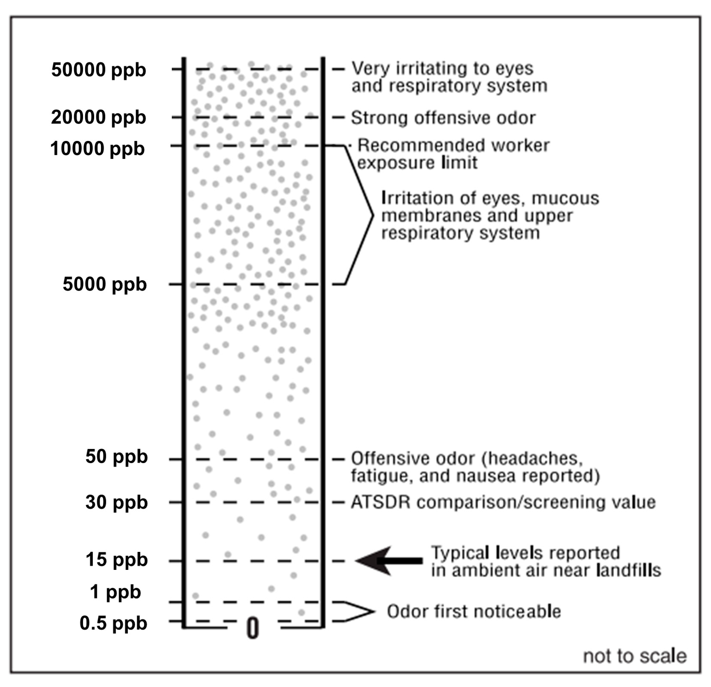
:1. Introduction
2. Materials and Methods
2.1. Measurements Period and Methods
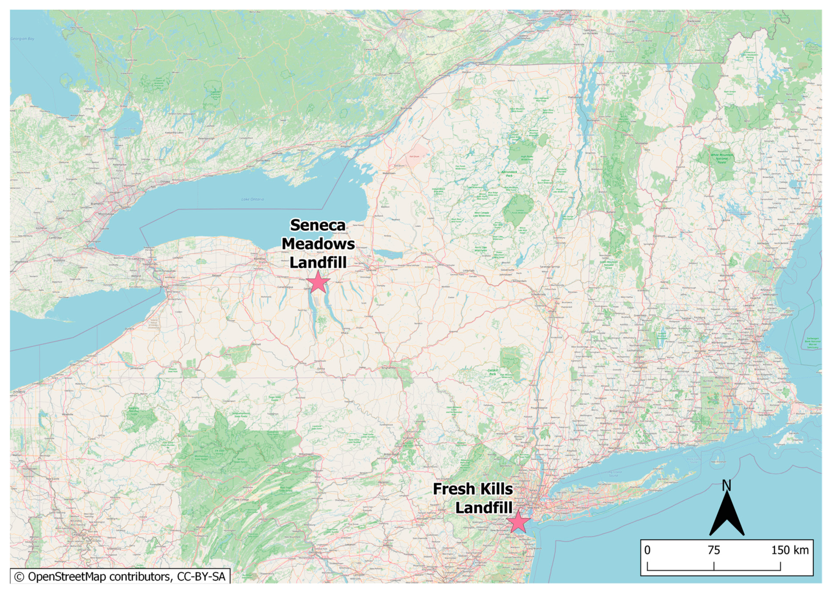
2.2. Measurement Locations (Landfills)
2.3. Data Analysis
3. Results and Discussion
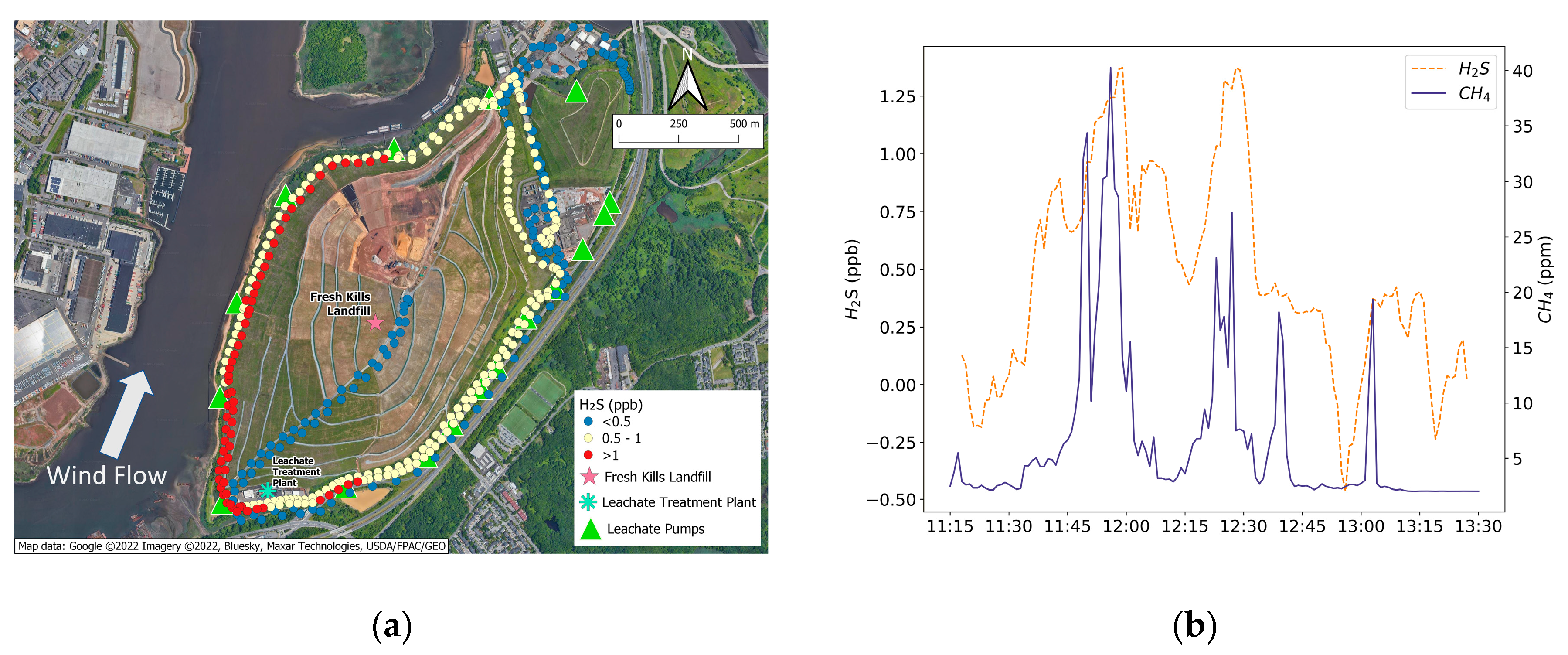
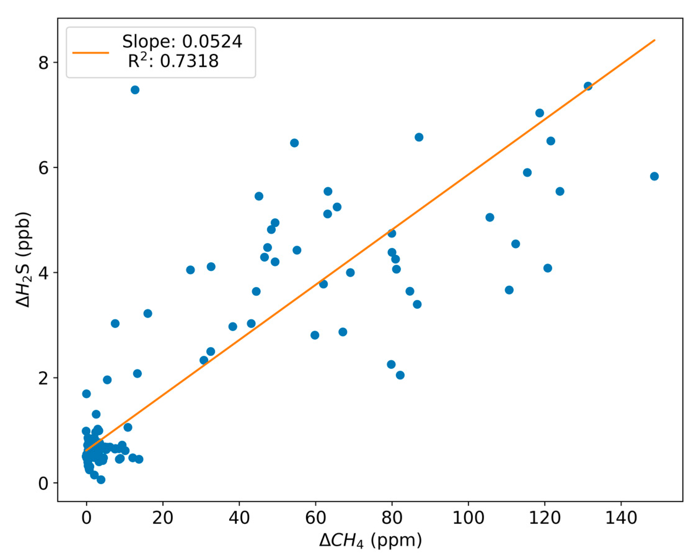
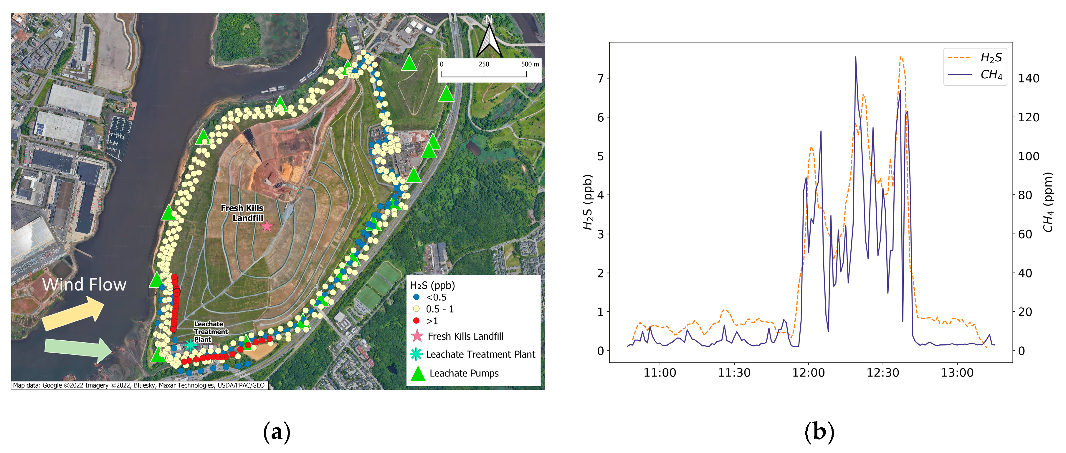
3.1. Landfill-Dependent H2S Mixing Ratio, ΔH2S/ΔCH4 Ratio, and Emission Flux at Fresh Kills Landfill
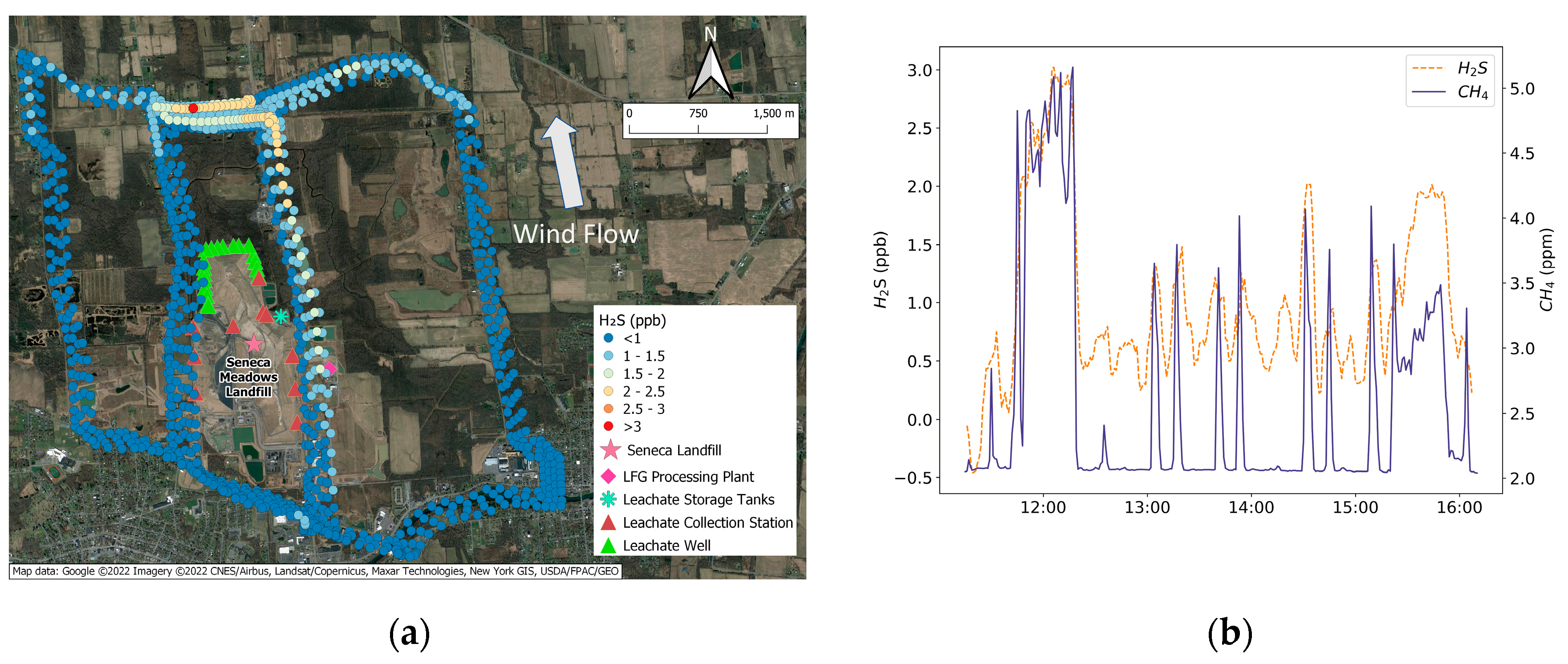
3.2. Landfill-Dependent H2S Concentration, ΔH2S/ΔCH4 Ratio, and Emission Flux at Seneca Meadows Landfill
3.3. Comparisons with Previous Work at Landfills
4. Conclusions
Author Contributions
Funding
Institutional Review Board Statement
Informed Consent Statement
Data Availability Statement
Acknowledgments
Conflicts of Interest
References
- Kurniawan, T.A.; Liang, X.; Singh, D.; Othman, M.H.D.; Goh, H.H.; Gikas, P.; Kern, A.O.; Kusworo, T.D.; Shoqeir, J.A. Harnessing Landfill Gas (LFG) for Electricity: A Strategy to Mitigate Greenhouse Gas (GHG) Emissions in Jakarta (Indonesia). J. Environ. Manag. 2022, 301, 113882. [Google Scholar] [CrossRef]
- United States Environmental Protection Agency. Basic Information about Landfill Gas. Available online: https://www.epa.gov/lmop/basic-information-about-landfill-gas (accessed on 16 July 2022).
- Lim, S.Y.; Lim, K.M.; Yoo, S.H. External Benefits of Waste-to-Energy in Korea: A Choice Experiment Study. Renew. Sustain. Energy Rev. 2014, 34, 588–595. [Google Scholar] [CrossRef]
- Heaney, C.D.; Wing, S.; Campbell, R.L.; Caldwell, D.; Hopkins, B.; Richardson, D.; Yeatts, K. Relation between Malodor, Ambient Hydrogen Sulfide, and Health in a Community Bordering a Landfill. Environ. Res. 2011, 111, 847–852. [Google Scholar] [CrossRef] [Green Version]
- Xu, Q.; Townsend, T. Factors Affecting Temporal H2S Emission at Construction and Demolition (C&D) Debris Landfills. Chemosphere 2014, 96, 105–111. [Google Scholar] [CrossRef] [PubMed]
- Long, Y.; Fang, Y.; Shen, D.; Feng, H.; Chen, T. Hydrogen Sulfide (H2S) Emission Control by Aerobic Sulfate Reduction in Landfill. Sci. Rep. 2016, 6, 38103. [Google Scholar] [CrossRef] [PubMed]
- Sakawi, Z.; Mastura, S.a.; Jaafar, O.; Mahmud, M.; Centre, E.O. Community Perception of Odor Pollution from the Landfill. GEOGRAFIA Online Malays. J. Soc. Space 2011, 7, 18–23. [Google Scholar]
- Ko, J.H.; Xu, Q.; Jang, Y.C. Emissions and Control of Hydrogen Sulfide at Landfills: A Review. Crit. Rev. Environ. Sci. Technol. 2015, 45, 2043–2083. [Google Scholar] [CrossRef]
- National Overview: Facts and Figures on Materials, Wastes and Recycling|US EPA. Available online: https://www.epa.gov/facts-and-figures-about-materials-waste-and-recycling/national-overview-facts-and-figures-materials#Trends1960-Today (accessed on 20 June 2022).
- Martuzzi, M.; Mitis, F.; Forastiere, F. Inequalities, Inequities, Environmental Justice in Waste Management and Health. Eur. J. Public Health 2010, 20, 21–26. [Google Scholar] [CrossRef]
- Kim, K.H.; Choi, Y.; Jeon, E.; Sunwoo, Y. Characterization of Malodorous Sulfur Compounds in Landfill Gas. Atmos. Environ. 2005, 39, 1103–1112. [Google Scholar] [CrossRef]
- Kim, K.H.; Jeon, E.C.; Choi, Y.J.; Koo, Y.S. The Emission Characteristics and the Related Malodor Intensities of Gaseous Reduced Sulfur Compounds (RSC) in a Large Industrial Complex. Atmos. Environ. 2006, 40, 4478–4490. [Google Scholar] [CrossRef]
- Ying, D.; Chuanyu, C.; Bin, H.; Yueen, X.; Xuejuan, Z.; Yingxu, C.; Weixiang, W. Characterization and Control of Odorous Gases at a Landfill Site: A Case Study in Hangzhou, China. Waste Manag. 2012, 32, 317–326. [Google Scholar] [CrossRef] [PubMed]
- Kim, K.H. Emissions of Reduced Sulfur Compounds (RSC) as a Landfill Gas (LFG): A Comparative Study of Young and Old Landfill Facilities. Atmos. Environ. 2006, 40, 6567–6578. [Google Scholar] [CrossRef]
- He, R.; Xia, F.F.; Bai, Y.; Wang, J.; Shen, D.S. Mechanism of H2S Removal during Landfill Stabilization in Waste Biocover Soil, an Alterative Landfill Cover. J. Hazard Mater. 2012, 217–218, 67–75. [Google Scholar] [CrossRef] [PubMed]
- United States Environmental Protection Agency. Best Management Practices to Prevent and Control Hydrogen Sulfide and Reduced Sulfur Compound Emissions at Landfills That Dispose of Gypsum Drywall; Environmental Protection Agency: Federal Triangle, WA, USA, 2014.
- ATSDR. Health Consultation—Ambient Airborne Exposures to Hydrogen Sulfide and Particulate Matter. Available online: https://www.atsdr.cdc.gov/HAC/pha/IndustrialPipeInc/Industrial_Pipe_Inc_EI-HC_08-21-2017_508.pdf (accessed on 20 June 2022).
- National Research Council (US). Hydrogen Sulfide Acute Exposure Guideline Levels—Acute Exposure Guideline Levels for Selected Airborne Chemicals—NCBI Bookshelf; National Academies Press: Cambridge, MA, USA, 2010; Volume 9. [Google Scholar]
- Reiffenstein, R.J.; Hulbert, W.C.; Roth, S.H. Toxicology of Hydrogen Sulfide. Annu. Rev. Pharmacol. Toxicol 2003, 32, 109–134. [Google Scholar] [CrossRef]
- ATSDR. Landfill Gas Primer—Chapter 3 Continued: What do We Know about the Potential Health Effects of Exposure to Landfill Gas? Available online: https://www.atsdr.cdc.gov/HAC/landfill/html/ch3a.html (accessed on 18 July 2022).
- United States Environmental Protection Agency. Emission Factor Documentation for AP-42 Section 2.4 Municipal Solid Waste Landfills. Available online: https://www3.epa.gov/ttn/chief/ap42/ch02/bgdocs/b02s04.pdf (accessed on 20 June 2022).
- Themelis, N.J.; Ulloa, P.A. Methane Generation in Landfills. Renew. Energy 2007, 32, 1243–1257. [Google Scholar] [CrossRef]
- Myhre, G.; Shindell, D.; Bréon, F.; Collins, W.; Fuglestvedt, J.; Huang, J.; Koch, D.; Lamarque, J.; Lee, D.; Mendoza, B.; et al. Anthropogenic and Natural Radiative Forc-Ing. In Climate Change 2013: The Physical Science Basis. Contribution of Working Group I; Cambridge University Press: Cambridge, UK, 2013. [Google Scholar]
- New York State Department of Environmental Conservation. Summary Report 2021 NYS Statewide GHG Emissions Report. Available online: https://www.dec.ny.gov/docs/administration_pdf/ghgsumrpt21.pdf (accessed on 27 June 2022).
- ASTDR. Toxicological Profile for Hydrogen Sulfide and Carbonyl Sulfide; U.S. Department of Health and Human Services, Public Health Service: Atlanta, GA, USA, 2016.
- Zhang, J.; Lance, S.; Marto, J.; Sun, Y.; Ninneman, M.; Crandall, B.A.; Wang, J.; Zhang, Q.; Schwab, J.J. Evolution of Aerosol Under Moist and Fog Conditions in a Rural Forest Environment: Insights From High-Resolution Aerosol Mass Spectrometry. Geophys. Res. Lett. 2020, 47, e2020GL089714. [Google Scholar] [CrossRef]
- Zhang, J.; Ninneman, M.; Joseph, E.; Schwab, M.J.; Shrestha, B.; Schwab, J.J. Mobile Laboratory Measurements of High Surface Ozone Levels and Spatial Heterogeneity During LISTOS 2018: Evidence for Sea Breeze Influence. J. Geophys. Res. Atmos. 2020, 125, 31961. [Google Scholar] [CrossRef]
- G2204 Analyzer Datasheet|Picarro. Available online: https://www.picarro.com/support/library/documents/g2204_analyzer_datasheet (accessed on 28 June 2022).
- The City of New York Department of Sanitation. NYC Sanitation, NYC Parks and NYS Department of Environmental Conservation Announce Final Certification of Fresh Kills Landfill Closure. Available online: https://www1.nyc.gov/assets/dsny/site/resources/press-releases/nyc-sanitation-nyc-parks-and-nys-department-of-environmental-conservation-announce-final-certification-of-fresh-kills-landfill-closure (accessed on 27 June 2022).
- United States Environmental Protection Agency. Determination of Landfill Gas Composition and Pollutant Emission Rates at Fresh Kills Landfill; National Service Center for Environmental Publications: Cincinnati, OI, USA; Volume 1, p. 272.
- New York State Department of Environmental Conservation. Permit Review Report: NYCDOS Fresh Kills Landfill. Permit ID: 2-6499-00029/00151. Available online: https://www.dec.ny.gov/dardata/boss/afs/permits/prr_264990002900151_r3.pdf (accessed on 27 June 2022).
- New York State Department of Environmental Conservation. Air Title V Facility Permit: Seneca Meadows Inc. Permit ID: 8-4532-00023/00041. Available online: https://www.dec.ny.gov/dardata/boss/afs/permits/prr_845320002300041_r2_4.pdf (accessed on 27 June 2022).
- New York State Department of Environmental Conservation. 2019 MSW Landfill Capacity Chart. Available online: https://www.dec.ny.gov/chemical/23723.html (accessed on 27 June 2022).
- CFR. eCFR :: 40 CFR Part 258—Criteria for Municipal Solid Waste Landfills. Available online: https://www.ecfr.gov/current/title-40/chapter-I/subchapter-I/part-258 (accessed on 27 June 2022).
- Brotzge, J.A.; Wang, J.; Thorncroft, C.D.; Joseph, E.; Bain, N.; Bassill, N.; Farruggio, N.; Freedman, J.M.; Hemker, K.; Johnston, D.; et al. A Technical Overview of the New York State Mesonet Standard Network. J. Atmos. Ocean. Technol. 2020, 37, 1827–1845. [Google Scholar] [CrossRef]
- Monteiro, V.C.; Miles, N.L.; Richardson, S.J.; Barkley, Z.; Haupt, B.J.; Lyon, D.; Hmiel, B.; Davis, K.J. Methane, Carbon Dioxide, Hydrogen Sulfide, and Isotopic Ratios of Methane Observations from the Permian Basin Tower Network. Earth Syst. Sci. Data 2022, 14, 2401–2417. [Google Scholar] [CrossRef]
- Conley, S.; Faloona, I.; Mehrotra, S.; Suard, M.; Lenschow, D.H.; Sweeney, C.; Herndon, S.; Schwietzke, S.; Pétron, G.; Pifer, J.; et al. Application of Gauss’s Theorem to Quantify Localized Surface Emissions from Airborne Measurements of Wind and Trace Gases. Atmos. Meas. Tech. 2017, 10, 3345–3358. [Google Scholar] [CrossRef] [Green Version]
- Schwietzke, S.; Harrison, M.; Lauderdale, T.; Branson, K.; Conley, S.; George, F.C.; Jordan, D.; Jersey, G.R.; Zhang, C.; Mairs, H.L.; et al. Aerially Guided Leak Detection and Repair: A Pilot Field Study for Evaluating the Potential of Methane Emission Detection and Cost-Effectiveness. J. Air Waste Manag. Assoc. 2018, 69, 71–88. [Google Scholar] [CrossRef] [PubMed]
- United States Environmental Protection Agency Office of Atmospheric Programs. Greenhouse Gas Reporting Program (GHGRP) [FLIGHT]. Available online: https://www.epa.gov/ghgreporting/ (accessed on 27 June 2022).
- CFR. eCFR :: 40 CFR Part 98 Subpart HH—Municipal Solid Waste Landfills. Available online: https://www.ecfr.gov/current/title-40/chapter-I/subchapter-C/part-98/subpart-HH#p-98.343 (accessed on 16 July 2022).
- United States Environmental Protection Agency. Municipal Solid Waste Landfills Subpart HH, Greenhouse Gas Reporting Program. Available online: https://www.epa.gov/sites/default/files/2018-02/documents/hh_infosheet_2018.pdf (accessed on 15 July 2022).
- Parker, T.; Dottridge, J.; Kelly, S. Investigation of the Composition and Emissions of Trace Components in Landfill Gas—R&D Technical Report; Environmental Agency: Bristol, UK, 2002.
- Naveen, B.P.; Mahapatra, D.M.; Sitharam, T.G.; Sivapullaiah, P.v.; Ramachandra, T.v. Physico-Chemical and Biological Characterization of Urban Municipal Landfill Leachate. Environ. Pollut. 2017, 220, 1–12. [Google Scholar] [CrossRef] [PubMed]
- Bergersen, O.; Haarstad, K. Metal Oxides Remove Hydrogen Sulfide from Landfill Gas Produced from Waste Mixed with Plaster Board under Wet Conditions. J. Air Waste Manag. Assoc. 2008, 58, 1014–1021. [Google Scholar] [CrossRef] [PubMed]
- Ren, X.; Salmon, O.E.; Hansford, J.R.; Ahn, D.; Hall, D.; Benish, S.E.; Stratton, P.R.; He, H.; Sahu, S.; Grimes, C.; et al. Methane Emissions From the Baltimore-Washington Area Based on Airborne Observations: Comparison to Emissions Inventories. J. Geophys. Res. Atmos. 2018, 123, 8869–8882. [Google Scholar] [CrossRef]
- Foster, C.S.; Crosman, E.T.; Holland, L.; Mallia, D.V.; Fasoli, B.; Bares, R.; Horel, J.; Lin, J.C. Confirmation of Elevated Methane Emissions in Utah’s Uintah Basin With Ground-Based Observations and a High-Resolution Transport Model. J. Geophys. Res. Atmos. 2017, 122, 13026–13044. [Google Scholar] [CrossRef]
- Lavoie, T.N.; Shepson, P.B.; Cambaliza, M.O.L.; Stirm, B.H.; Karion, A.; Sweeney, C.; Yacovitch, T.I.; Herndon, S.C.; Lan, X.; Lyon, D. Aircraft-Based Measurements of Point Source Methane Emissions in the Barnett Shale Basin. Environ. Sci. Technol. 2015, 49, 7904–7913. [Google Scholar] [CrossRef] [Green Version]
- Lyon, D.R.; Zavala-Araiza, D.; Alvarez, R.A.; Harriss, R.; Palacios, V.; Lan, X.; Talbot, R.; Lavoie, T.; Shepson, P.; Yacovitch, T.I.; et al. Constructing a Spatially Resolved Methane Emission Inventory for the Barnett Shale Region. Environ. Sci. Technol. 2015, 49, 8147–8157. [Google Scholar] [CrossRef] [Green Version]
- Guha, A.; Newman, S.; Fairley, D.; Dinh, T.M.; Duca, L.; Conley, S.C.; Smith, M.L.; Thorpe, A.K.; Duren, R.M.; Cusworth, D.H.; et al. Assessment of Regional Methane Emission Inventories through Airborne Quantification in the San Francisco Bay Area. Environ. Sci. Technol 2020, 2020, 9264. [Google Scholar] [CrossRef]
- Colledge, M.A. Estimating Impacts of Hydrogen Sulfide Gas Emissions From a Construction and Demolition Debris Landfill. Ph.D. Thesis, University of Illinois, Champaign, IL, USA, 1996. [Google Scholar]
- Eun, S.; Reinhart, D.R.; Cooper, C.D.; Townsend, T.G.; Faour, A. Hydrogen Sulfide Flux Measurements from Construction and Demolition Debris (C&D) Landfills. Waste Manag. 2007, 27, 220–227. [Google Scholar] [CrossRef]
- Mønster, J.; Kjeldsen, P.; Scheutz, C. Methodologies for Measuring Fugitive Methane Emissions from Landfills—A Review. Waste Manag. 2019, 87, 835–859. [Google Scholar] [CrossRef]
- Fang, J.J.; Yang, N.; Cen, D.Y.; Shao, L.M.; He, P.J. Odor Compounds from Different Sources of Landfill: Characterization and Source Identification. Waste Manag. 2012, 32, 1401–1410. [Google Scholar] [CrossRef] [PubMed]
- Song, S.K.; Shon, Z.H.; Kim, K.H.; Cheon Kim, S.; Kim, Y.K.; Kim, J.K. Monitoring of Atmospheric Reduced Sulfur Compounds and Their Oxidation in Two Coastal Landfill Areas. Atmos. Environ. 2007, 41, 974–988. [Google Scholar] [CrossRef]
- Lee, S.; Xu, Q.; Booth, M.; Townsend, T.G.; Chadik, P.; Bitton, G. Reduced Sulfur Compounds in Gas from Construction and Demolition Debris Landfills. Waste Manag. 2006, 26, 526–533. [Google Scholar] [CrossRef] [PubMed]
- Shon, Z.H.; Kim, K.H.; Jeon, E.C.; Kim, M.Y.; Kim, Y.K.; Song, S.K. Photochemistry of Reduced Sulfur Compounds in a Landfill Environment. Atmos. Environ. 2005, 39, 4803–4814. [Google Scholar] [CrossRef]
- Vasarevičius, S. Investigation and Evaluation of H2S Emissions from a Municipal Landfill. J. Environ. Eng. Landsc. Manag. 2011, 19, 12–20. [Google Scholar] [CrossRef]
- de La Rosa, D.A.; Velasco, A.; Rosas, A.; Volke-Sepúlveda, T. Total Gaseous Mercury and Volatile Organic Compounds Measurements at Five Municipal Solid Waste Disposal Sites Surrounding the Mexico City Metropolitan Area. Atmos. Environ. 2006, 40, 2079–2088. [Google Scholar] [CrossRef]
- Font, R.; Carratalá, A.; Edo, M.; Munoz, M. Distribution of Hydrogen Sulfide, Ammonia and Volatile Compounds in the Ambient Air Surrounding a Landfill Facility. Chem. Eng. Trans. 2010, 23, 225–230. [Google Scholar] [CrossRef]
- Calace, N.; Liberatori, A.; Petronio, B.M.; Pietroletti, M. Characteristics of Different Molecular Weight Fractions of Organic Matter in Landfill Leachate and Their Role in Soil Sorption of Heavy Metals. Environ. Pollut. 2001, 113, 331–339. [Google Scholar] [CrossRef]
- Widdel, F. Microbiology and Ecology of Sulfate-and Sulfur-Reducing Bacteria, 99th ed.; Zehnder, A.J.B., Ed.; Wiley-Interscience: Hoboken, NJ, USA, 1988. [Google Scholar]
- Fredenslund, A.M.; Scheutz, C.; Kjeldsen, P. Tracer Method to Measure Landfill Gas Emissions from Leachate Collection Systems. Waste Manag. 2010, 30, 2146–2152. [Google Scholar] [CrossRef]
- Thompson, M.A.; Kelkar, U.G.; Vickers, J.C. The Treatment of Groundwater Containing Hydrogen Sulfide Using Microfiltration. Desalination 1995, 102, 287–291. [Google Scholar] [CrossRef]


| Study | Type of Landfill/Location | H2S Emission Flux Estimate mg m−2 Day−1 |
|---|---|---|
| This study | MSW/Fresh Kills Landfill, NY, USA | 0.02 ± 0.01 * |
| This study | MSW/Seneca Meadows Landfill, NY, USA | 17.7 ± 12.9 ** 5.1 ± 2.6 * |
| EPA (1995) [30] | MSW/Fresh Kills Landfill, NY, USA | Entire landfill: 0.08–10497.6 Section 1/9 cell: 0.19–10.94 |
| Eun et al. (2007) [51] | C&D/multiple landfills in Florida, USA | 0.192–1.76 |
| Xu et al. (2014) [5] | C&D/Orlando, Florida, USA | 0.40–1.07 |
| Colledge et al. (2008) [50] | C&D/Warren Recycling Landfill in Ohio, USA | 19.01–210.82 |
| Study | Type of Landfill/Location | Sampling Month (s) | Measurement Method | Measured H2S Mixing Ratios |
|---|---|---|---|---|
| This Study | MSW/NY, USA | November | Continuous mobile measurements | 1.3–7 ppb |
| Heaney et al., 2011 [4] | Regional MSW/NC, USA | January–February, September–November | Continuous monitoring at fence line | 0–14.86 ppb |
| EPA (1995) [30] | MSW/Fresh Kills Landfill, NY, USA | June and July | Passive vents, flux chamber measurements, and gas collection system measurements at Section 1/9 cell of the landfill | Entire landfill 0.11–220 ppm Section 1/9 5.3–35 ppm |
| Parker et al., 2002 [42] | MSW/co-disposal site, United Kingdom | September and March | LFG sampling from gas wells | 1.2–5.4 ppm |
| Shon et al., 2005 [56] | MSW/Daegu landfill, S. Korea | January | Ambient air sampling at the entrance of landfill, along the border, and center | 0.026–27.01 ppb |
| Fang et al., 2012 [53] | MSW/Shanghai, China | May | Ambient air sampling | 2.9–109 ppb |
| Vasarevicius, 2011 [57] | MSW/Jerubaiciai landfill, Plunge district, Lithuania | August, November, February, April | Ambient air sampling from equidistant points over the landfill | (Highest amounts) Aug—8.6 ppm Nov—8.1 ppm Feb—6.0 ppm Apr—7.3 ppm |
| Kim, 2006 [14] | MSW/Dong Hae, S. Korea | May, July, November, and December | LFG venting pipe | (Measured area <5 years old) May—2.6–124.4 ppm July—6.8–523.8 ppm Nov—0.44–281.0 ppm Dec—70.3–181.3 ppm (Measured area 5–23 years old) May—0.0002–0.002 ppm July—0.00055 ppm Nov—0.0013–0.005 ppm |
| de la Rosa et al., 2006 [58] | MSW/Mexico City, MX | September–November | Sampling from drilled holes in the cover and vent | ~18–150 ppm |
| Font et al., 2010 [59] | Valencianne Community, Spain | July and November | July—3.6–16.3 ppb Nov—2.5–8.8 ppb | Ambient air sampling |
| Song et al., 2007 [54] | MSW/S. Korea | May, July, August, October, and December | Ambient air sampling | 0.046–5.396 ppb |
| Lee et al., 2006 [55] | 10 C&D Landfills/ Florida, USA | NA | Ambient air sampling | 0.003–50 ppm |
| Colledge et al. (2008) [50] | C&D/Warren Recycling Landfill in Ohio, USA | October–September, June–August | Continuous ambient air sampling | 0–178 ppb |
| Ratio (mol mol−1) | R2 | |
|---|---|---|
| Fresh Kills Day 2 | 5.2 ± 2.6 × 10⁻⁵ | ~0.7 |
| Seneca | 8.6 ± 4.3 × 10⁻⁴ | ~0.7 |
Publisher’s Note: MDPI stays neutral with regard to jurisdictional claims in published maps and institutional affiliations. |
© 2022 by the authors. Licensee MDPI, Basel, Switzerland. This article is an open access article distributed under the terms and conditions of the Creative Commons Attribution (CC BY) license (https://creativecommons.org/licenses/by/4.0/).
Share and Cite
Catena, A.M.; Zhang, J.; Commane, R.; Murray, L.T.; Schwab, M.J.; Leibensperger, E.M.; Marto, J.; Smith, M.L.; Schwab, J.J. Hydrogen Sulfide Emission Properties from Two Large Landfills in New York State. Atmosphere 2022, 13, 1251. https://doi.org/10.3390/atmos13081251
Catena AM, Zhang J, Commane R, Murray LT, Schwab MJ, Leibensperger EM, Marto J, Smith ML, Schwab JJ. Hydrogen Sulfide Emission Properties from Two Large Landfills in New York State. Atmosphere. 2022; 13(8):1251. https://doi.org/10.3390/atmos13081251
Chicago/Turabian StyleCatena, Alexandra M., Jie Zhang, Roisin Commane, Lee T. Murray, Margaret J. Schwab, Eric M. Leibensperger, Joseph Marto, Mackenzie L. Smith, and James J. Schwab. 2022. "Hydrogen Sulfide Emission Properties from Two Large Landfills in New York State" Atmosphere 13, no. 8: 1251. https://doi.org/10.3390/atmos13081251
APA StyleCatena, A. M., Zhang, J., Commane, R., Murray, L. T., Schwab, M. J., Leibensperger, E. M., Marto, J., Smith, M. L., & Schwab, J. J. (2022). Hydrogen Sulfide Emission Properties from Two Large Landfills in New York State. Atmosphere, 13(8), 1251. https://doi.org/10.3390/atmos13081251