Abstract
The electric field data of ELF/VLF frequency bands recorded by space Electric Field Detector (EFD) on satellite CSES were utilized to analyze the abnormal electromagnetic (EM) emission associated with seismic activities. Two adjacent earthquakes (EQ), which are the Mw6.9 EQ on 7 July and the Mw7.2 EQ on 14 July 2019 in Indonesia, were selected as examples. The disturbance of the electric field in the ELF/VLF band was extracted by using observational and comparative analysis methods. The results of this study indicate the following. (1) The significant electric field anomalies in the ELF/VLF band (mainly from about 49 to 366 Hz) were detected near the epicenter, exactly in the northeast, of two strong low-latitude earthquakes by the electric field detector of CSES. (2) The electric field disturbances were mainly detected by satellite CSES over the epicenters at night, i.e., along the ascending orbits. (3) These abnormal enhancements will gradually diminish as the frequency increases. (4) The electric field anomalies started to appear in the northeast of the epicenters before the mainshocks and gradually moved closer to the sources after them. At the same time, a clear magnetically conjugated feature also gradually appeared before the first earthquake, but then faded away when approaching the next one.
1. Introduction
Earthquakes are common geological disasters in nature, which seriously threaten the safety of human life and property. The occurrence of earthquakes is a procession of accumulating stress to sudden fracture and displacement of lithosome, and rapid release of energy to produce seismic waves. The electromagnetic emission is also considered as a small part of this massive energy of an earthquake. For decades, numerous abnormal EM emissions, ranging from direct current (DC) to tens of kilohertz and even up to high frequencies, associated with seismic activities during the preparation or co-seismic period were recorded by the ground- and space-based instruments [1,2,3,4,5,6,7,8,9,10,11,12].
Due to the low-frequency, electromagnetic waves can penetrate through the waveguide and lower ionosphere and then be observed by a low Earth orbit (LEO) satellite [13,14]. In recent years, the space-based or satellite-based detection has become an important method to detect the electromagnetic wave radiated from earthquakes. In 2004, the DEMETER (Detection of Electromagnetic Emissions Transmitted from Earthquake Regions) satellite [15] was launched to detect ionospheric perturbations [16]. Case [6,10,17,18,19] and statistical [7,8,20] studies have since reported obvious seismic electromagnetic emissions by using DEMETER observations. Recently, the newly launched China Seismo–Electromagnetic Satellite (CSES, also known as ZhangHeng-1) [21] has also been used to monitor and study seismo–ionospheric perturbations [9,11,22]. In order to better use the CSES data, Zhao et al. [23] have constructed a lithosphere–atmosphere–ionosphere coupling model to estimate the detection capability of electromagnetic payloads of the CSES to electromagnetic signals induced by strong earthquakes. However, more CSES-based observations are needed to obtain a more accurate EM field distribution at satellite altitudes for seismic anomaly studies and cross-validate with theoretical models. In this paper, we used the electric field data of the CSES to analyze possible abnormal electromagnetic emission associated with seismic activities and provide case support and a theoretical basis for earthquake monitoring.
2. Data Acquisition and Pre-Processing
2.1. The EFD Data
The CSES was successfully launched on 2 February 2018, with EFD as one of the main payloads [21,24]. EFD can provide basic data for the study of Solar-terrestrial space physics, space weather, ionosphere, upper atmosphere, magnetosphere and other related interactions and effects, and provide data for research on seismic observation research. The scheme used in the detection is a dual-probe type, which is based on the source and characteristics of the space electric field in the earth’s ionosphere. The design is based on the principle: apply the bias current to the spherical probe and on the premise of reducing the impedance of the plasma sheath of the probe, the potential of the double spherical probe in the space of ionosphere is obtained. The data for the electric field along the line direction is obtained by dividing the difference of the potentials between the two probes by the distance between the probes. Errors in the detected data are mainly caused by solar irradiation and the applied bias current. The detection frequency band of the load is divided into DC~ULF (0~16 Hz), ULF~ELF (6~2.2 kHz) and ELF~VLF (1.8~20 kHz). The results of a large number of earthquakes show that the disturbance before and during earthquake may affect the propagation of high-power radio signals in the ELF~VLF band.
2.2. The Earthquake Information
In this paper, two shallow earthquakes with magnitudes greater than 6.0 and source depths less than 50 km in Indonesia were selected. The seismic parameters are shown in detail in Table 1. According to Dobrovolsky formula , and here, M is the magnitude [25], the radius of the seismogenic zone of earthquake No. 1 is about 926.83 km, and that of earthquake No. 2 is about 1247.38 km.

Table 1.
The information of two earthquakes.
2.3. Data Pre-Processing
According to previous research [26], it is believed that the electromagnetic wave radiated from the seismogenic zone propagates along the magnetic field line, so the ionospheric disturbance recorded by satellite is not directly above the epicenter but has a certain deviation. Therefore, a space window with the epicenter was selected.
Data pre-processing is mainly divided into the two following steps to eliminate the influence of possible electromagnetic background noise as much as possible:
- (1)
- Select the nighttime orbits that passing over the epicenters, namely the ascending orbits. Due to possible weak ionospheric disturbances caused by earthquake may be influenced by the solar radiation environment, the nighttime data were analyzed in this paper.
- (2)
- Considering the potential impact of solar and geomagnetic activities, a stringent condition (, and ) was set for selecting quiet period. The perturbation of the ionosphere caused by solar activity and interplanetary magnetic field is much greater than that caused by the movement of the earth’s crust. Therefore, only the orbital data during the quiet period were selected for analysis in this paper.
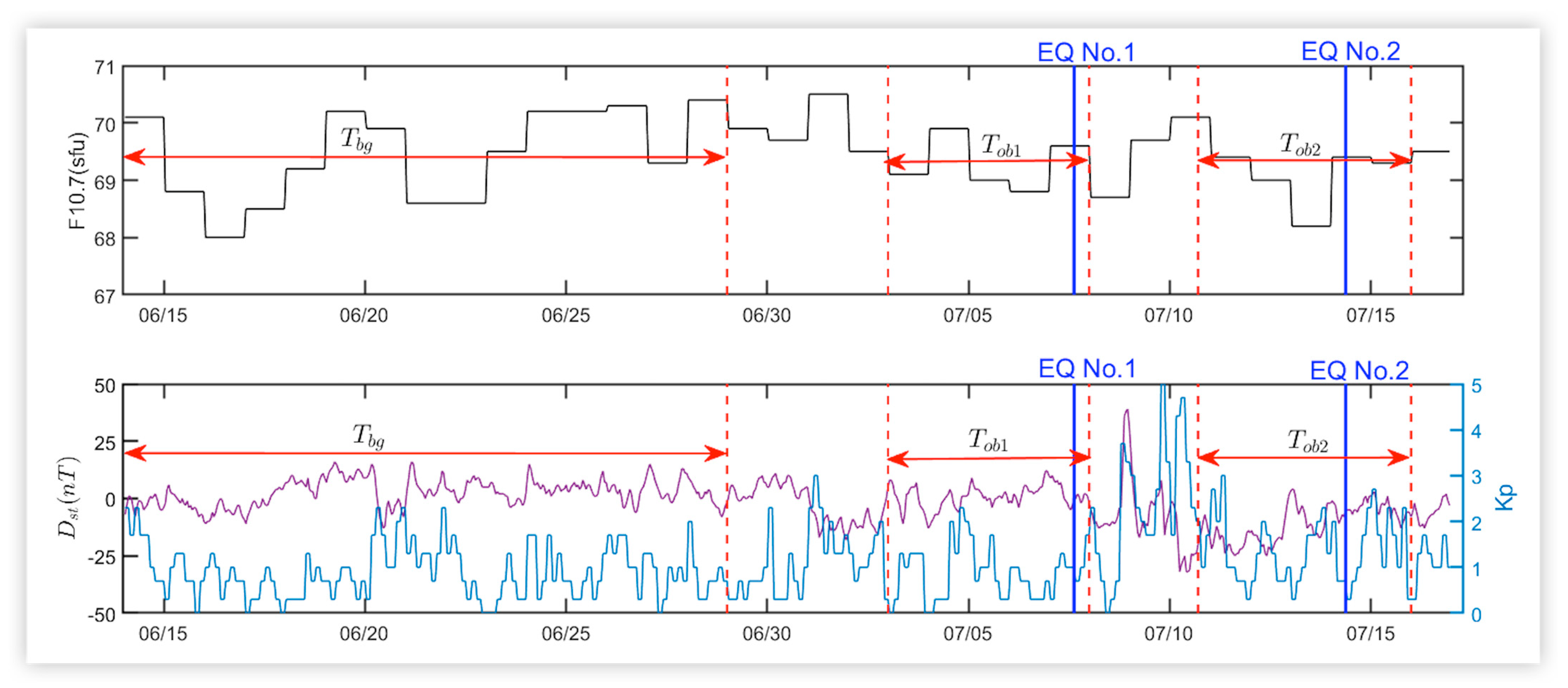
Figure 1 illustrates the levels of F10.7, Dst and Kp from 14 June to 15 July, namely the time interval from three weeks before case No. 1 to one day after case No. 2. As shown in the figure, the background data and the observation data of the two earthquakes used in this paper are both in quiet period.
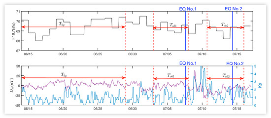
Figure 1.
The levels of indexes F10.7, Dst and Kp. is the time interval of the background data, and and are the observed intervals for case No. 1 and No. 2, respectively. The blue vertical lines illustrate the time of the main shocks.
3. Methodology and Results
The frequency range of electromagnetic disturbances generated by earthquakes is from DC to high frequency [1,2,3,5]. Due to the low attenuation of the low frequency (ULF, ELF, and VLF) currents in the propagation, it is easier to be observed by low Earth orbit satellites before and after earthquakes. For example, the electric field disturbance before the earthquake observed by the DEMETER satellite in the frequency range of 39–80 Hz [27], and the enhancement of magnetic field intensity at 100, 216, and 467 Hz observed by the OGO-6 satellite [28]. Usually, the frequency range of seismo–ionospheric electromagnetic disturbance occurs below 500 Hz, and often manifests as signal enhancement. Therefore, the data of power spectral density (PSD) of the electric field at single frequency points were selected as observational data for comparative analysis. Due to the five-day revisit period of CSES, the time span of the selected observational data for each case is five days.
3.1. Analysis of Observed Values
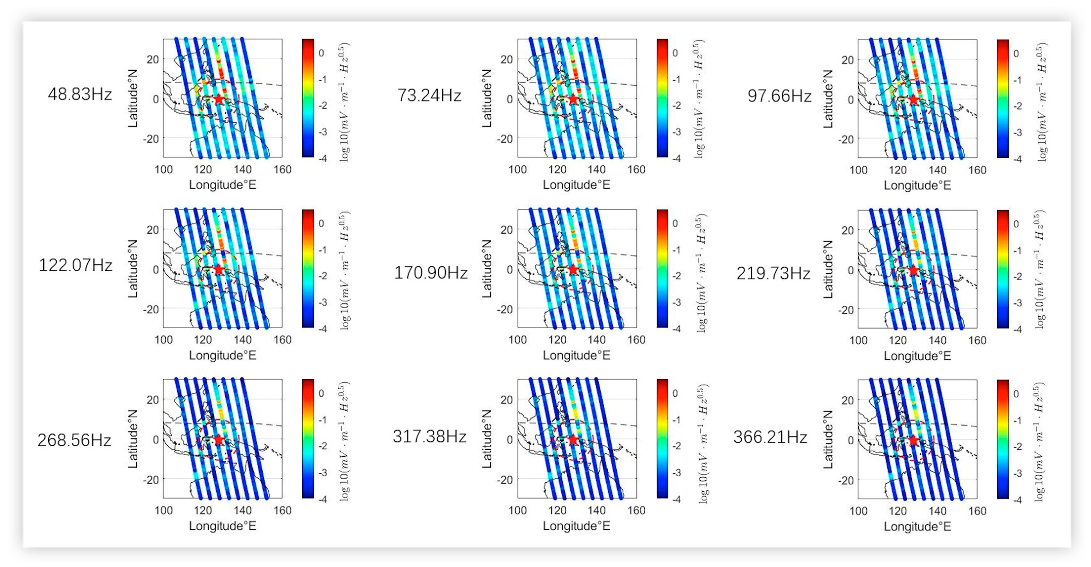
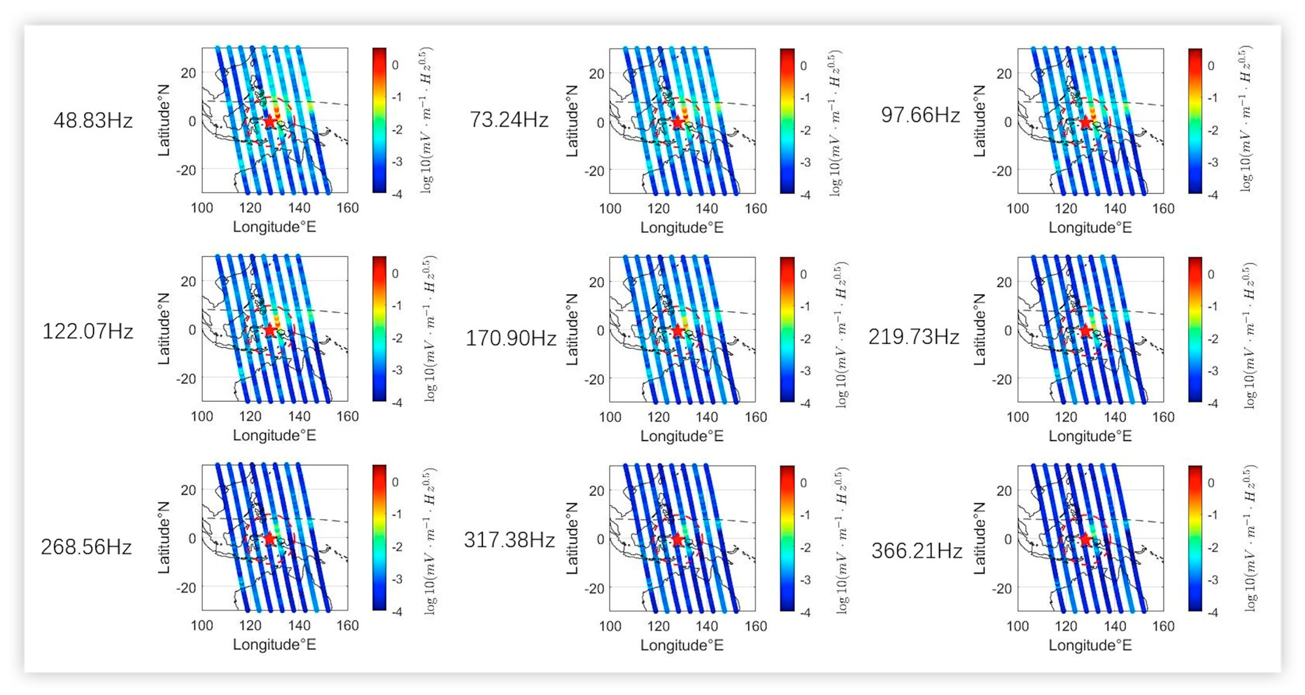
For earthquake No. 1, the ascending orbit passing over the epicenter from four days before to one day after the earthquake, i.e., 4 July to 8 July (as seen in Figure 1), was selected as the observation orbit to make the distribution map for PSD at the single frequency points. Each subfigure in Figure 2 represents the distribution of PSD of the electric field corresponding to different single frequency point.
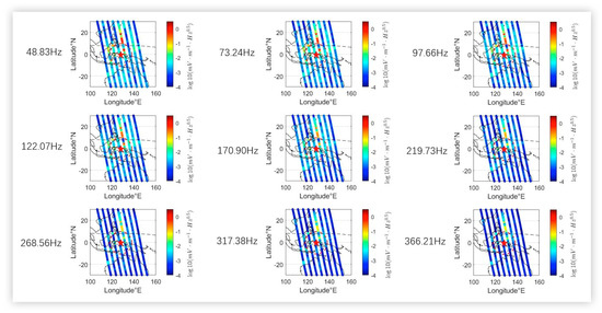
Figure 2.
Using the earthquake No. 1 as the object, the distribution of observational values of PSD of the electric field on the ascending orbits from 4 July to 8 July. From left to right, the dotted lines indicate the satellite trajectories on 8, 4, 5, 6, 7, 8, 4, and 5 July. The red stars, dashed circles, and black dashed curves indicate the epicenters of two earthquakes, the estimated seismogenic zones, and the magnetic equators, respectively.
As seen in Figure 2, the abnormal enhancements were found over the epicenter. In particular, the values of PSD over the epicenter drastically enhanced up to 2–3 orders of magnitude higher than background values on the ascending orbit passing over the seismogenic zone on 7 July (about two hours after the shock time of case No. 1), namely semi-orbit 07911_1. Meanwhile, this feature gradually diminishes as the frequency increases. In detail, these enhancements are mainly concentrated in 3° N to 20° N along the semi-orbit 07911_1. However, there exists a gap near 7° N, which is close to the magnetic equator, then results in this kind of magnetically conjugated distribution.
For earthquake No. 2, similarly, we also selected the revisit orbits from four days before to one day after the earthquake as the observational period, i.e., 11 July to 15 July (as seen in Figure 1). Figure 3 shows the electric field PSD distribution of the single frequency point. As seen in Figure 3, the similar enhancements, up to 2–3.5 orders of magnitude higher than background values, mainly occurred on the ascending orbit passing through the seismogenic zone on 12 July (two days before the shock time of case No. 2), namely semi-orbit 07987_1. Likewise, this feature also gradually diminishes as the frequency increases. However, these enhancements are mainly localized in 0° N to 6° N, which are entirely within the seismogenic zone and closer to the epicenter, along the semi-orbit 07987_1.
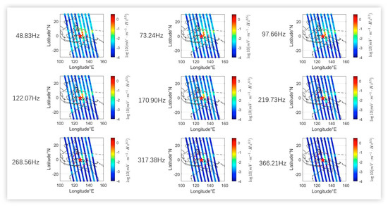
Figure 3.
Similar to Figure 2, using the earthquake No. 2 as the object, the distribution of observational values of PSD of the electric field on the ascending orbits during 11 July to 15 July. From left to right, the dotted lines indicate the satellite trajectories on 13, 14, 15, 11, 12, 13, 14 and 15 July, respectively.
3.2. Analysis of Relative Values
In Section 3.1, the significant electric field disturbances were detected from actual satellite observation data along the ascending orbits (in the nighttime) passing over the epicenters. In order to confirm the anomalous signals mentioned above and exclude the spatial background disturbance, a comparative analysis was introduced.
Due to the epicenters and onset-time of these two earthquakes being close to each other, in that sense, the possible interaction effects need to be taken into account. Finally, the nighttime data of ascending orbits passing over the epicenters from 14 June to 28 June, during the solar and geomagnetic quiet period, were selected as background data. Then, we defined the relative values as follows. (1) Centered on each data sampling point () on the observation orbits, a square window with 3° × 3° (Longitude × Latitude) was set. (2) All nighttime data (ascending orbits) were accumulated when the satellite passes through this window during the entire background period, i.e., 14 to 28 June (as seen in Figure 1). (3) The average as the background value () was obtained for this data sampling point. (4) was set as the relative value for each sampling point along these ascending orbits.
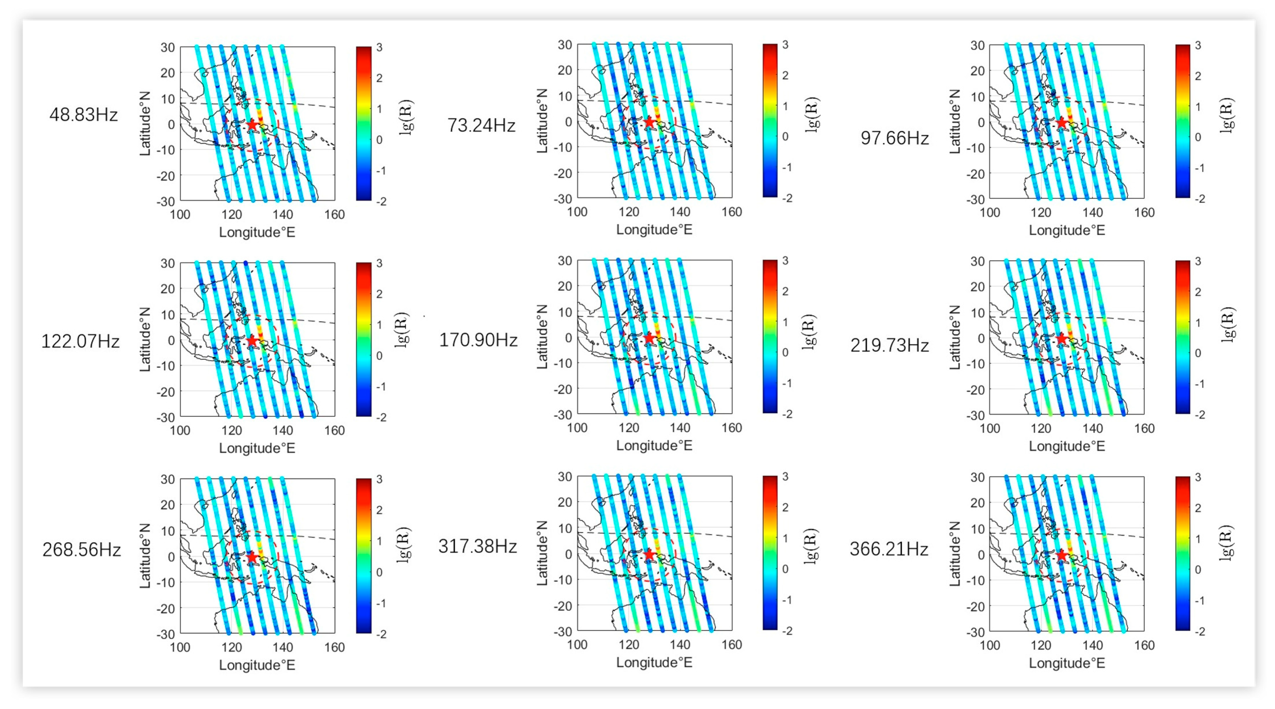
Figure 4 represents the relative PSD values of the electric field on the ascending orbits passing over the epicenter of earthquake No. 1. The same is shown in with Figure 2, where the anomalies still exist over the epicenter. Similarly, the relative values of the electric field PSD over the earthquake seismogenic zone drastically enhanced up to 1–3 orders of magnitude higher on the ascending semi-orbit 07911_1 (7 July). It is worth noting that this phenomenon also gradually weakens as the frequency increases, but not as obvious as in the observations.
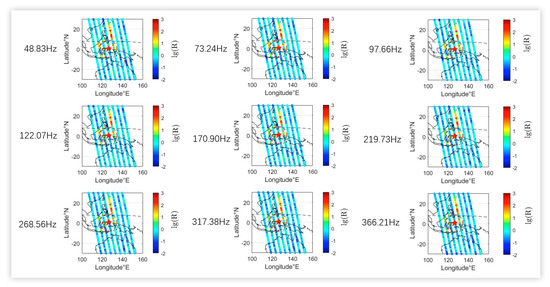
Figure 4.
Using the earthquake No. 1 as the object, the relative values of the electric field PSD on ascending orbits from 4 July to 8 July. From left to right, the dotted lines indicate the satellite trajectories on 8, 4, 5, 6, 7, 8, 4, and 5 July, respectively. The red stars, dashed circles and black dashed curves indicate the epicenters of two earthquakes, the estimated seismogenic zones and the magnetic equators, respectively.
A comparable situation occurred for earthquake No. 2; the anomalies of relative values, up to 1.5–3.5 orders of magnitude higher than the background, mainly occurred on the ascending semi-orbit 07987_1 passing through the earthquake seismogenic zone on 12 July (as shown in Figure 5). When the frequency increases, this feature has a significant tendency to diminish. Meanwhile, the enhancements are also localized within the earthquake seismogenic zone and close to the epicenter.
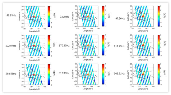
Figure 5.
Similar to Figure 4, using the earthquake No. 2 as the object, the relative values of the electric field PSD on ascending orbits from 11 July to 15 July. From left to right, the dotted lines indicate the satellite trajectories on 13, 14, 15, 11, 12, 13, 14, and 15 July, respectively.
3.3. The Two-Dimensional Spatial Distribution
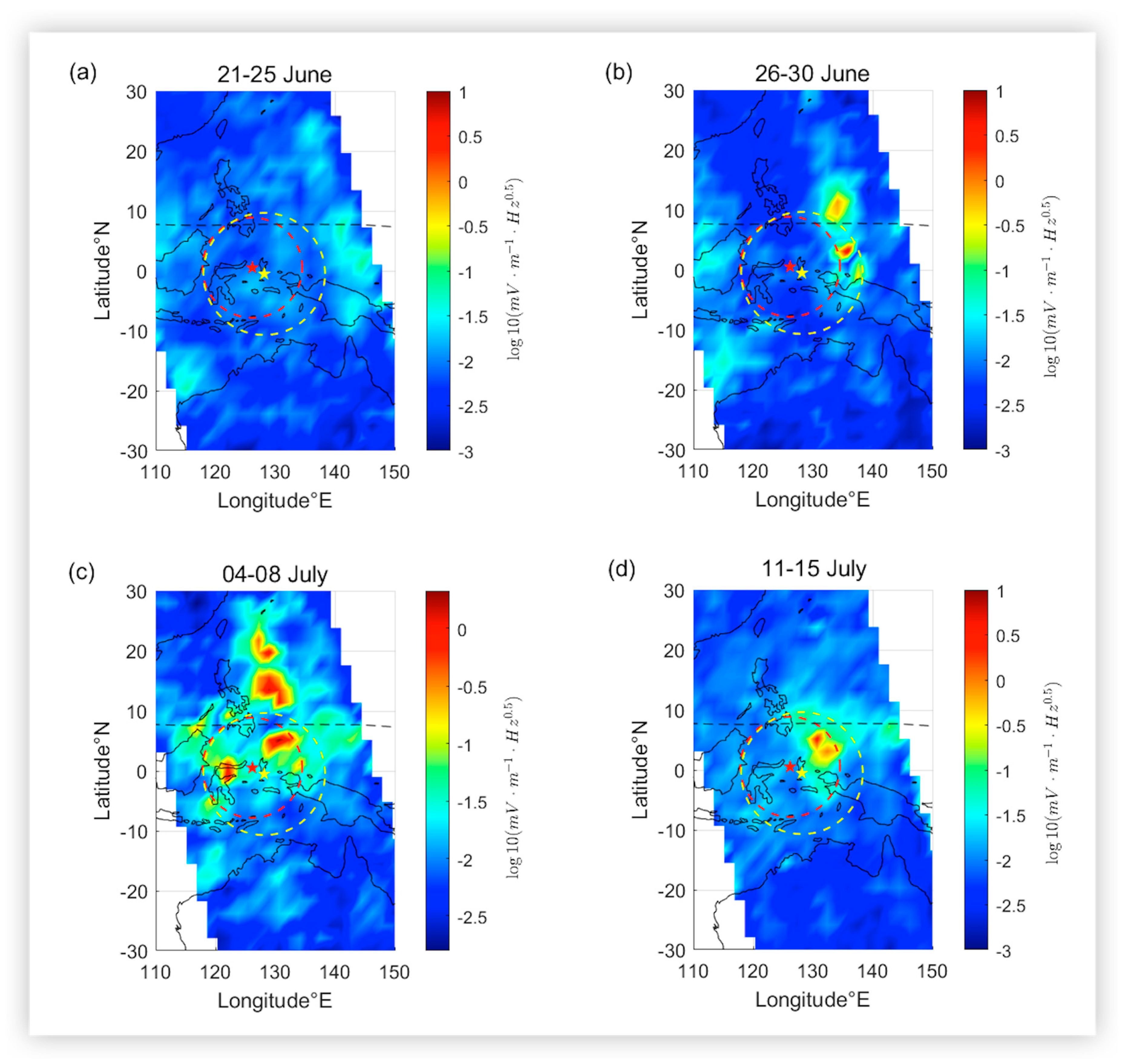
Furthermore, in order to more clearly observe the spatial movement characteristics of the anomaly areas, which may be corresponding with two adjacent strong earthquakes, a two-dimensional spatial distribution map was also built with the observational data of the electric field PSD at frequency 48 Hz (as seen in Figure 6). In detail, we used the values, combining with spatial interpolation algorithms, on all ascending orbits (nighttime) passing over the estimated seismogenic zones within every five days from 16 days before earthquakes No. 1. As seen in Figure 6a, the level of the electric field disturbance over the earthquake was very low from 21 to 25 June, and then the anomalies began to appear in the northeast of the epicenters and gradually moved closer to the sources. In particular, a clear magnetically conjugated feature also appeared (as seen in Figure 6b,c) and then faded away when approaching Earthquake No. 2, and it was consistent with the results depicted in Figure 2 and Figure 4.
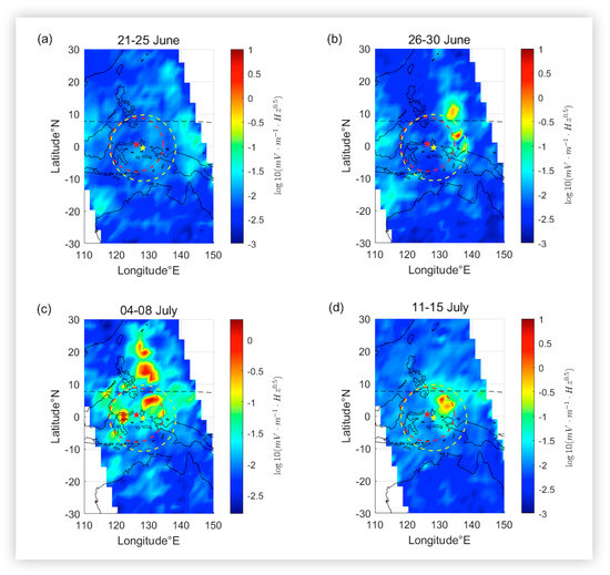
Figure 6.
The two-dimensional distribution map for the PSD of the electric field at frequency 48 Hz. The results during the period: (a) from 21 to 25 June, (b) from 26 to 30 June, (c) from 4 to 8 July and (d) from 11 to 15 July, respectively. The red (yellow) stars and dashed circles indicate the epicenters and estimated seismogenic zones of earthquake No. 1 (No. 2), respectively. The black dashed curves illustrate the magnetic equators.
4. Discussion
In this paper, we attempt to critically analyze the ionospheric electric field disturbance during the strong earthquakes. From the above results, it is clear that the electric field PSD both enhances abnormally near the epicenter, exactly in the northeast, of two strong earthquakes and these kinds of features will gradually diminish as the frequency increases. These anomalies appear to be associated with these strong earthquakes. However, it should be noted that it is difficult to classify exactly which disturbances are directly related to which earthquake, because the epicenters and onset-time of these two earthquakes are close to each other. In addition, it is difficult to completely eliminate the possible background noise due to natural non-seismic (such as thunderstorms and volcanic eruptions, etc.) or artificial (such as powerful man-made VLF transmitters and power line harmonic radiation, etc.) sources of electromagnetic emissions, although stringent solar and geomagnetic conditions (i.e., , and ) have been adopted during the analysis process. Nevertheless, the difficulties of this work should be recognized and approached with caution in detecting seismo–ionospheric anomalies.
The significant EM anomalies in the ELF/VLF band, from about 49 to 366 Hz, were detected by the electric field detector of CSES. In detail, the electric field enhances abnormally over the epicenter during two strong seismic activities, which suggests that the low frequency EM waves can penetrate through the waveguide and lower ionosphere and then be detected by LEO satellite [13,14,29]. The piezoelectric effect [30,31,32] or electrokinetic effect [33,34] can be used to explain the possible physical mechanisms of seismically excited EM signals. Recently, in order to estimate the detection capability of EM payloads of CSES to EM signals induced by strong seismic activities, Zhao et al. [23] also constructed a lithosphere–atmosphere–ionosphere coupling model for ELF radio wave propagation. In their simulated results, the EM anomalies radiating from strong earthquake (M > 6.0) can be detected by the EM sensor of the CSES, although there are some factors to consider, such as the focal depth, the current moment of the source and the lithosphere conductivity, etc. Meanwhile, the electric field disturbances were mainly detected by satellite CSES at night, i.e., along the ascending orbits. However, we also checked the data on the descending ones in the daytime but no similar anomalies were found. This may be caused by the fact that the electric field at night are higher than those in the daytime because of the lower electron density and collisions at night. In addition, these kinds of features, i.e., abnormal enhancements, will gradually diminish as the frequency increases. Due to lower frequency, waves have longer wavelengths with less attenuation due to conductivity, namely the skin effect [23].
Interestingly, a clear magnetically conjugated feature gradually appeared before the first earthquake, as seen in Figure 6, and then faded away when approaching the next one. In some ways, it could be explained by the mechanism of seismic–atmosphere–ionosphere–magnetosphere coupling, i.e., seismo–electromagnetic emissions can propagate as Alfven waves along the geomagnetic lines [35,36,37,38,39]. However, it is worth recognizing that two epicenters in this paper are in a low-latitude region and near to the magnetic equator, thus the fountain effect should be considered.
5. Conclusions
In this paper, the electric field data recorded by space Electric Field Detector (EFD) on satellite CSES were utilized to analyze the phenomenon of ELF/VLF emission disturbances during two strong shallow earthquakes near the equator. We attempted to critically analyze the satellite-based detection of electromagnetic signals induced by strong earthquakes. The main results of this study are summarized below.
- (1)
- The significant electric field anomalies in the ELF/VLF band (mainly from about 49 to 366 Hz) were detected near the epicenter, exactly in the northeast, of two strong low-latitude earthquakes by the electric field detector of CSES.
- (2)
- The electric field disturbances were mainly detected by satellite CSES over the epicenters at night, i.e., along the ascending orbits.
- (3)
- These abnormal enhancements will gradually diminish as the frequency increases.
- (4)
- The electric field anomalies started to appear in the northeast of the epicenters before the mainshocks and gradually moved closer to the sources after them. At the same time, a clear magnetically conjugated feature also gradually appeared before the first earthquake, but then faded away when approaching the next one.
In order to establish a reasonable electromagnetic wave coupling mechanism to obtain a more accurate EM field distribution at satellite altitudes for seismic anomaly studies, more satellite-based observations need to be cross-validated with theoretical models in the future.
Author Contributions
Conceptualization, D.T.; methodology, J.Z. and D.T.; software, J.Z. and D.T.; validation, J.Z. and D.T.; formal analysis, J.Z. and D.T.; investigation, J.Z. and D.T.; resources, J.Z. and D.T.; data curation, J.Z. and D.T.; writing—original draft preparation, J.Z.; writing—review and editing, D.T.; visualization, J.Z. and D.T.; supervision, D.T. and X.S.; project administration, D.T.; funding acquisition, D.T. All authors have read and agreed to the published version of the manuscript.
Funding
This work is supported by the National Natural Science Foundation of China (Grant No. 42004137) and the Natural Science Foundation of Sichuan Province of China (Grant No. 2022NSFSC0213).
Institutional Review Board Statement
Not applicable.
Informed Consent Statement
Not applicable.
Data Availability Statement
The earthquake data are available at https://earthquake.usgs.gov/earthquakes (accessed on 28 August 2022) and CSES electric field data are accessible from www.leos.ac.cn (accessed on 15 July 2022).
Acknowledgments
This work made use of the data from the CSES mission, a project funded by the China National Space Administration (CNSA) and the China Earthquake Administration (CEA). We thank the CSES satellite team for the data. We also acknowledge the National Earthquake Information Center (NEIC) ComCat database of the US Geological Survey for providing available earthquake data.
Conflicts of Interest
The authors declare no conflict of interest.
References
- Gokhberg, M.B.; Morgounov, V.A.; Yoshino, T.; Tomizawa, I. Experimental Measurement of Electromagnetic Emissions Possibly Related to Earthquakes in Japan. J. Geophys. Res. 1982, 87, 7824. [Google Scholar] [CrossRef]
- Sorokin, V.; Chmyrev, V.; Yaschenko, A. Electrodynamic Model of the Lower Atmosphere and the Ionosphere Coupling. J. Atmos. Sol.-Terr. Phys. 2001, 63, 1681–1691. [Google Scholar] [CrossRef]
- Hayakawa, M. VLF/LF Radio Sounding of Ionospheric Perturbations Associated with Earthquakes. Sensors 2007, 7, 1141–1158. [Google Scholar] [CrossRef]
- Pulinets, S.; Ouzounov, D. Lithosphere-Atmosphere-Ionosphere Coupling (LAIC) Model—An Unified Concept for Earthquake Precursors Validation. J. Asian Earth Sci. 2011, 41, 371–382. [Google Scholar] [CrossRef]
- Huang, Q. Rethinking Earthquake-Related DC-ULF Electromagnetic Phenomena: Towards a Physics-Based Approach. Nat. Hazards Earth Syst. Sci. 2011, 11, 2941–2949. [Google Scholar] [CrossRef]
- Zhima, Z.; Shen, X.; Zhang, X.; Cao, J.; Huang, J.; Ouyang, X.; Jing, L.; Lu, B. Possible Ionospheric Electromagnetic Perturbations Induced by the Ms7.1 Yushu Earthquake. Earth Moon Planets 2012, 108, 231–241. [Google Scholar] [CrossRef]
- Zhang, X.; Shen, X.; Parrot, M.; Zeren, Z.; Ouyang, X.; Liu, J.; Qian, J.; Zhao, S.; Miao, Y. Phenomena of Electrostatic Perturbations before Strong Earthquakes (2005–2010) Observed on DEMETER. Nat. Hazards Earth Syst. Sci. 2012, 12, 75–83. [Google Scholar] [CrossRef]
- Zhang, X.; Fidani, C.; Huang, J.; Shen, X.; Zeren, Z.; Qian, J. Burst Increases of Precipitating Electrons Recorded by the DEMETER Satellite before Strong Earthquakes. Nat. Hazards Earth Syst. Sci. 2013, 13, 197–209. [Google Scholar] [CrossRef]
- Zhou, B.; Yang, Y.; Zhang, Y.; Gou, X.; Cheng, B. Magnetic Field Data Processing Methods of the China Seismo-Electromagnetic Satellite. Earth Planet. Phys. 2018, 2, 455–461. [Google Scholar] [CrossRef]
- Zhima, Z.; Hu, Y.; Piersanti, M.; Shen, X.; Guo, F. The Seismic Electromagnetic Emissions During the 2010 Mw 7.8 Northern Sumatra Earthquake Revealed by DEMETER Satellite. Front. Earth Sci. 2020, 8, 572393. [Google Scholar] [CrossRef]
- Wang, Q.; Huang, J.; Zhao, S.; Zhima, Z.; Yan, R.; Lin, J.; Yang, Y.; Chu, W.; Zhang, Z.; Lu, H. The Electromagnetic Anomalies Recorded by CSES during Yangbi and Madoi Earthquakes Occurred in Late May 2021 in West China—ScienceDirect. Nat. Hazards Res. 2022, 2, 1–10. [Google Scholar] [CrossRef]
- Li, Z.; Yang, B.; Huang, J.; Yin, H.; Yang, X.; Liu, H.; Zhang, F.; Lu, H. Analysis of Pre-Earthquake Space Electric Field Disturbance Observed by CSES. Atmosphere 2022, 13, 934. [Google Scholar] [CrossRef]
- Cohen, M.B.; Inan, U.S. Terrestrial VLF Transmitter Injection into the Magnetosphere. J. Geophys. Res.-Space Phys. 2012, 117, A08310. [Google Scholar] [CrossRef]
- Zhao, S.; Zhou, C.; Shen, X.; Zhima, Z. Investigation of VLF Transmitter Signals in the Ionosphere by ZH-1 Observations and Full-Wave Simulation. J. Geophys. Res.-Space Phys. 2019, 124, 4697–4709. [Google Scholar] [CrossRef]
- Lagoutte, D.; Brochot, J.; de Carvalho, D.; Elie, F.; Harivelo, F.; Hobara, Y.; Madrias, L.; Parrot, M.; Pincon, J.; Berthelier, J.; et al. The DEMETER Science Mission Centre. Planet. Space Sci. 2006, 54, 428–440. [Google Scholar] [CrossRef]
- Parrot, M.; Benoist, D.; Berthelier, J.; Blecki, J.; Chapuis, Y.; Colin, F.; Elie, F.; Fergeau, P.; Lagoutte, D.; Lefeuvre, F.; et al. The Magnetic Field Experiment IMSC and Its Data Processing Onboard DEMETER: Scientific Objectives, Description and First Results. Planet. Space Sci. 2006, 54, 441–455. [Google Scholar] [CrossRef]
- Bertello, I.; Piersanti, M.; Candidi, M.; Diego, P.; Ubertini, P. Electromagnetic Field Observations by the DEMETER Satellite in Connection with the 2009 L’Aquila Earthquake. Ann. Geophys. 2018, 36, 1483–1493. [Google Scholar] [CrossRef]
- Bhattacharya, S.; Sarkar, S.; Gwal, A.K.; Parrot, M. Satellite and Ground-Based ULF/ELF Emissions Observed before Gujarat Earthquake in March 2006. Curr. Sci. 2007, 93, 41–46. [Google Scholar]
- Walker, S.N.; Kadirkamanathan, V.; Pokhotelov, O.A. Changes in the Ultra-Low Frequency Wave Field during the Precursor Phase to the Sichuan Earthquake: DEMETER Observations. Ann. Geophys. 2013, 31, 1597–1603. [Google Scholar] [CrossRef]
- Nemec, F.; Santolik, O.; Parrot, M. Decrease of Intensity of ELF/VLF Waves Observed in the Upper Ionosphere Close to Earthquakes: A Statistical Study. J. Geophys. Res.-Space Phys. 2009, 114, A04303. [Google Scholar] [CrossRef]
- Shen, X.H.; Zong, Q.G.; Zhang, X.M. Introduction to Special Section on the China Seismo-Electromagnetic Satellite and Initial Results. Earth Planet. Phys. 2018, 2, 439–443. [Google Scholar] [CrossRef]
- Wen, Y.Z.; Tao, D.; Wang, G.X.; Zong, J.Y.; Cao, J.B.; Battiston, R.; Zeren, Z.M.; Shen, X.H. Ionospheric TEC and Plasma Anomalies Possibly Associated with the 14 July 2019 M_(w) 7.2 Indonesia Laiwui Earthquake, from Analysis of GPS and CSES Data. Earth Planet. Phys. 2022, 6, 16. [Google Scholar] [CrossRef]
- Zhao, S.; Shen, X.; Liao, L.; Zeren, Z. A Lithosphere-Atmosphere-Ionosphere Coupling Model for ELF Electromagnetic Waves Radiated from Seismic Sources and Its Possibility Observed by the CSES. Sci. China-Technol. Sci. 2021, 64, 2551–2559. [Google Scholar] [CrossRef]
- Huang, J.P.; Lei, J.G.; Li, S.X.; Zeren, Z.M.; Li, C.; Zhu, X.H.; Yu, W.H. The Electric Field Detector (EFD) Onboard the ZH-1 Satellite and Firstobservational Results. Earth Planet. Phys. 2018, 2, 10. [Google Scholar] [CrossRef]
- Dobrovolsky, I.P.; Zubkov, S.I.; Miachkin, V.I. Estimation of the Size of Earthquake Preparation Zones. Pure Appl. Geophys. 1979, 117, 1025–1044. [Google Scholar] [CrossRef]
- Pulinets, S. Ionospheric Precursors of Earthquakes; Recent Advances in Theory and Practical Applications. TAO Terr. Atmos. Ocean. Sci. 2004, 15, 413. [Google Scholar] [CrossRef]
- Yan Rui; Wang Lanwei; Hu Zhe; Liu Dapeng; Zhang Xingguo; Zhang Yu Ionospheric Disturbances before and after Strong Earthquakes Based on DEMETER Data. Acta Seismol. Sin. 2013, 35, 498–511.
- Serebryakova, O.N.; Bilichenko, S.V.; Chmyrev, V.M.; Parrot, M.; Rauch, J.L.; Lefeuvre, F.; Pokhotelov, O.A. Electromagnetic ELF Radiation from Earthquake Regions as Observed by Low-altitude Satellites. Geophys. Res. Lett. 2013, 19, 91–94. [Google Scholar] [CrossRef]
- Lehtinen, N.G.; Inan, U.S. Full-Wave Modeling of Transionospheric Propagation of VLF Waves. Geophys. Res. Lett. 2009, 36, L03104. [Google Scholar] [CrossRef]
- Nitsan; Uzi Electromagnetic Emission Accompanying Fracture of Quartz-Bearing Rocks. Geophys. Res. Lett. 1977, 4, 333–336. [CrossRef]
- Ikeya, M.; Takaki, S.; Matsumoto, H.; Tani, A.; Komatsu, T. Pulsed Charge Model of Fault Behavior Producing Seismic Electric Signals (SES). J. Circuits Syst. Comput. 1997, 7, 153–164. [Google Scholar] [CrossRef]
- Huang, Q. One Possible Generation Mechanism of Co-Seismic Electric Signals. Proc. Jpn. Acad. Ser. B-Phys. Biol. Sci. 2002, 78, 173–178. [Google Scholar] [CrossRef] [Green Version]
- Mizutani, H.; Ishido, T.; Yokokura, T.; Ohnishi, S. Electrokinetic Phenomena Associated with Earthquakes. Geophys. Res. Lett. 1976, 3, 365–368. [Google Scholar] [CrossRef]
- Johnston, M. Review of Electric and Magnetic Fields Accompanying Seismic and Volcanic Activity. Surv. Geophys. 1997, 18, 441–476. [Google Scholar] [CrossRef]
- Aleksandrin, S.Y.; Galper, A.M.; Grishantzeva, L.A.; Koldashov, S.V.; Voronov, S.A. High-Energy Charged Particle Bursts in the near-Earth Space as Earthquake Precursors. Ann. Geophys. 2003, 21, 597–602. [Google Scholar] [CrossRef]
- Sgrigna, V.; Carota, L.; Conti, L.; Corsi, M.; Galper, A.M.; Koldashov, S.V.; Murashov, A.M.; Picozza, P.; Scrimaglio, R.; Stagni, L. Correlations between Earthquakes and Anomalous Particle Bursts from SAMPEX/PET Satellite Observations. J. Atmos. Sol.-Terr. Phys. 2005, 67, 1448–1462. [Google Scholar] [CrossRef]
- Liu, J.Y.; Chen, Y.I.; Chen, C.H.; Liu, C.Y.; Chen, C.Y.; Nishihashi, M.; Li, J.Z.; Xia, Y.Q.; Oyama, K.I.; Hattori, K. Seismoionospheric GPS Total Electron Content Anomalies Observed before the 12 May 2008 Mw7.9 Wenchuan Earthquake. J. Geophys. Res. Space Phys. 2009, 114, A04320. [Google Scholar] [CrossRef]
- Gulyaeva, T.L.; Arikan, F.; Stanislawska, I.; Poustovalova, L.V. Symmetry and Asymmetry of Ionospheric Weather at Magnetic Conjugate Points for Two Midlatitude Observatories. Adv. Space Res. 2013, 52, 1837–1844. [Google Scholar] [CrossRef]
- Tao, D.; Wang, G.; Zong, J.; Wen, Y.; Cao, J.; Battiston, R.; Zeren, Z. Are the Significant Ionospheric Anomalies Associated with the 2007 Great Deep-Focus Undersea Jakarta-Java Earthquake? Remote Sens. 2022, 14, 2211. [Google Scholar] [CrossRef]

Publisher’s Note: MDPI stays neutral with regard to jurisdictional claims in published maps and institutional affiliations. |
© 2022 by the authors. Licensee MDPI, Basel, Switzerland. This article is an open access article distributed under the terms and conditions of the Creative Commons Attribution (CC BY) license (https://creativecommons.org/licenses/by/4.0/).