Abstract
Using atmospheric data, which include pressure, temperature, relative humidity and water vapor pressure, the actual refractive index of a specific segment of the atmosphere has been modeled. Based on the refractive index, a numerical method is presented to quickly estimate the propagation path of the radio wave in the troposphere. Utilizing the terrain and the surface medium model of the propagation area and the parabolic equation (PE) method, an image of the electric field distribution of radio waves in the troposphere is obtained. A comparison of propagation paths between the numerical method and the PE model is presented. Additionally, the effects of the antenna’s elevation angle have been studied. Physical measurements provide a reference for the accuracy of the simulation results obtained using the method presented in this work.
1. Introduction
When a radio wave propagates in the troposphere, it is mainly impacted by the following three factors: terrain of the earth surface, medium on the earth surface (surface medium) and the meteorological condition. Terrain relates to the shape of the earth’s surface, which creates the scattering of radio waves. The surface medium refers to grinding attachments, which can be natural or artificial. While the natural objects include soil, water, and vegetation, the artificial attachments mainly refer to structures such as buildings and roads. The main effect of the surface medium is absorption and attenuation. Meteorological elements of the troposphere mainly include the pressure, temperature and relative humidity. The influence of meteorological elements affects the refractivity of the troposphere.
Some simplified numerical models have been proposed to indicate effects of the terrain [1,2,3,4,5] and surface medium [6,7,8,9] on radio waves propagation. With the rapid development of the geographic information system (GIS), complex terrain parameters can be obtained from digital maps. For example, elevation information can be extracted from the satellite map and is then converted into a digital elevation model (DEM) [10,11]. The color of the surface medium represent the reflection and absorption coefficient for electromagnetic (EM) waves. As a result, we can divide the areas with different colors in the high-definition (HD) satellite map into different media. Combined with the elevation information, the areas that have the same or similar colors but correspond to different media can be distinguished. Moreover, electromagnetic properties are assigned to different areas that have been categorized into different media. Therefore, taking into account these features, the influence of terrain and surface medium on radio waves’ propagation can be modeled.
Due to the atmospheric refraction caused by meteorological elements, radio waves do not travel in straight lines in the troposphere, thus leading to bending of the propagation path. For tracking the propagation paths of radio waves in the troposphere, analytical solutions are usually used [12,13], but the calculation process is complicated, and it is not easy to achieve a rapid estimation of propagation paths. A method was proposed in a previous study to calculate the effect of atmospheric refraction on the EM wave propagation path [14,15]. The proposed method can achieve fast prediction of the propagation path of EM waves by layering the atmosphere and combining it with Snell law. However, while the method provided a one-dimensional change of the propagation path of EM waves caused by atmospheric refraction, it fell short of giving the detailed distribution of EM waves in the propagation path.
In other works, empirical models of atmospheric refraction were used to simulate EM wave propagation in the troposphere [16,17]. In those models, the parabolic equations (PE) method was widely used [16,18,19,20,21]. However, in some applications, such as electronic warfare, wireless communication, and electromagnetic energy transfer, the PE modeling with its simplified assumptions would not be sufficient to provide sufficiently accurate and reliable results.
The refractive index of the troposphere can be derived from the pressure, temperature, relative humidity and water vapor pressure. Usually, it is a function of the elevation and remains constant over a considerable horizontal range. In this work, by substituting the actual refractive index of the troposphere into the PE method, combined with the terrain and the surface medium models, the tropospheric realistic propagation model of radio waves can be constructed. The model is able to present the field distribution of any profile on the propagation path. Furthermore, including information about the terrain and medium in the propagation region in the model enables the model to accurately predict the propagation characteristics of radio waves in real-world tropospheric environments. A comparison between the calculated results and the experimental results shows that the model has high computational accuracy. However, due to the limitation of computational resources and computational accuracy, the method is only applicable to the microwave and lower frequency bands.
2. Refractive Index from Atmospheric Sounding Data
2.1. Refractive Index
The troposphere is the first layer in the atmosphere closest to the ground. The troposphere properties are determined by meteorological conditions such as pressure, temperature, relative humidity (RH) and vapor pressure. These meteorological conditions affect the propagation of the radio wave in microwave frequency bands. The relative permittivity of the troposphere is given by [22,23,24]:
where p (hPa) is the atmospheric pressure, T is the temperature in K unite and e (hPa) is the vapor pressure, which can be derived from the relative humidity (RH) of the atmosphere [25]:
where indicates the saturated vapor pressure, which can be obtained from the following.
Usually, the difference between the troposphere classical refraction index n and 1 is very small; thus, for convenience, the refractivity is introduced. From (4), we have the following.
Some of the empirical models of the refractivity N are presented in [22], but the meteorological conditions vary depending on the area. In fact, from (2), (3) and (5), it is clear that the refractivity can be obtained as long as the tropospheric pressure, temperature and relative humidity are available. Therefore, if we can obtain the real-time atmospheric conditions of a specific area, the actual refractivity can be obtained. Fortunately, the Department of Atmospheric Science of Wyoming University has included real-time data from most of the world’s atmospheric sounding sites [26]. Consequently, we can substitute the related atmospheric sounding data into (2), (3) and (5) to obtain the actual refractivity versus height profile for any area of interest.
Taking the 2020 Chongqing of China as an example, we can obtain the refractivity N for selected days as Figure 1 shows. Note that the selected days represent four different seasons.
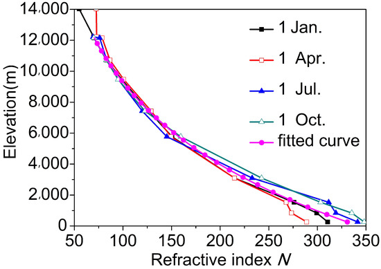
Figure 1.
The tropospheric refractivity of Chongqing for different seasons and the fitted curve.
According to the graphs of Figure 1, an average model of the tropospheric refractivity including seasonal information can be obtained, and a fitting expression can be obtained as follows:
where h (m) is the elevation.
2.2. Modified by the Curvature of the Earth
When the propagation distance in the horizontal direction is large enough (over-the-horizon, for example), the effect of the curvature of the Earth has to be considered. The influence of the curvature of the Earth can be achieved by modifying the refractivity of the troposphere. Refractivity can be modified as follows [22,27]:
where is the average radius of the Earth. According to Figure 1, the modified refractivity indices are provided in Figure 2, and a fitting expression can be also obtained as follow.
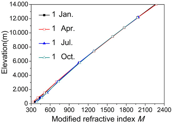
Figure 2.
The modified refractivity caused by the curvature of the Earth.
3. Propagation Path of the Radio Wave in Troposphere
It is often convenient to represent radiation as rays of energy instead of waves [22]. Owing to the refractivity of the troposphere, the propagation path of the radio wave will no longer be a straight line. The actual propagation path of the radio wave in the troposphere will help us understand the effects of meteorological conditions on radio waves. As Figure 3 shows, dividing the troposphere into layers, as long as the thickness of each layer is small enough, the refractive index of each layer can be treated as a constant. On the interface of layers, the angles of incidence and refraction satisfy Snell law:
where and are the incoming and outgoing incident angles, respectively. and are the refraction indexes of each layer of the troposphere.
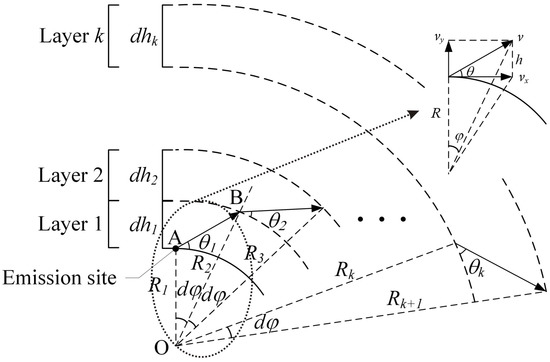
Figure 3.
Schematic diagram of the layered troposphere and propagation path of the radio wave.
The velocity of radio waves in any medium is , where c is the speed of light, and n is the refraction index. Thus, accordingly, the velocity in the horizontal and vertical directions of a radio wave traveling within the troposphere with an elevation angle can be written as follows.
After the elapse of , the radio wave would have propagated through many layers, and the opening angle at the center of the earth between the start and the end point of the propagation path can be obtained from the following:
where R is the sum of the radio source elevation and the average radius of the Earth, and is the travel distance in the vertical direction.
Based on the physics of propagation, the propagation path of the radio wave during each short time period () is determined by and . Due to the refractivity, n varies with elevation, which makes obtaining the analytical solution of (12) difficult. Therefore, we propose a numerical solution.
In Figure 3, the elevation angle of the radio wave is in the first layer. After a short period of time , it reaches point B, which is the start of the second layer.The opening angle at the center of the earth between points A and B is . By setting the refraction index of the layer 1 and 2 to and , respectively, the elevation angle of the radio wave at point B can be calculated by (9). From the trigonometric functions, the incidence angle in the triangle (see Figure 3) can be calculated by , while the refraction angle is . Therefore, combined with (9), we have the following.
The increasing distance in the vertical direction of point B is . Therefore, the elevation of point B can be obtained as follows:
where is the initial elevation of the radio source at point A (elevation from the earth’s surface), and can be obtained from (12) as follows.
The entire increasing distance of the radio wave in the vertical direction is , and the entire opening angle at the center of the Earth is . Thus, for a certain refractivity, the propagation path can be determined.
The elevation of the radio source was set to 700 m, and the total range (transmission distance in the horizontal direction) was set as 310 km. Since the propagation area includes two cities: Chongqing and Chengdu of China, the refractivity uses the average result of the two cities. The propagation paths of radio waves with different incident angles are provided in Figure 4.
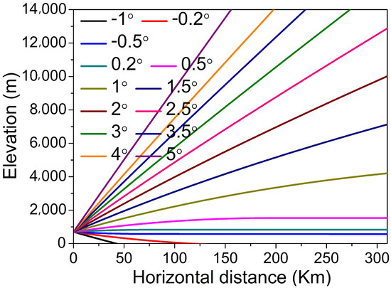
Figure 4.
The propagation paths of radio waves with different incident angle.
Due to the horizontal propagation distance that is 310 km, which is much longer than the over-the-horizon distance of 133.58 km ( km, m and m are the elevations where the transmitting and receiving antennas are located), the effect of the curvature of the Earth must be considered. Figure 5 shows the propagation paths when the Earth’s curvature is taken into account.
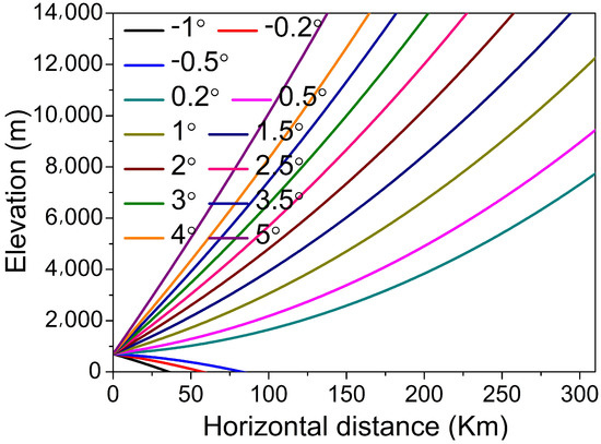
Figure 5.
Modified propagation paths of radio with the modified refractivity.
4. PE with Actual Refractivity
4.1. Overview of the PE Method
The PE method has been widely used to model the propagation of EM waves in complex atmospheric, hydrological, and geographical environments. Many wide-angle parabolic equation (WAPE) models have been proposed, which include the Claerbout PE method, Feit–Fleck PE modeling, and the Padé PE method. Among these models, the Feit–Fleck PE modeling is the most popular one [11].
Considering the scalar wave equations and assuming the time-dependence factor to be , we have the following:
where is the electric or magnetic field components, k is the free space wave number, and n is the refraction index. For 2D electromagnetic problems, (16) can be simplified into the following.
Assuming radio wave propagation along the x axis, the wave function can be written as . Substituting the wave function into (17), according to the paraxial condition, the scalar wave equation, in terms of u, can be expressed as follows.
By employing the Feit–Fleck approximation, a WAPE can be finally expressed as follows.
Next, the Slip-step Fourier Transform (SSFT) solution at of (19) can be acquired as follows [28]:
where and represent the Fourier and inverse Fourier transform, respectively, and is the angle measured with respect to the horizontal, is the range step, and is the initial field. The time-domain of the PE method can be obtained by Fourier synthesis.
As presented in Section 3, the tracing on the propagation path of a radio wave can only reflect the effect of tropospheric refraction but cannot give the distribution of the field, which would provide an important qualitative picture of the real propagation conditions. By substituting the actual refractivity and the real terrain model and the surface medium model into (20), the propagation properties of the radio waves in the troposphere of a specific area can be determined.
4.2. Calculation Conditions
Two identical parabolic antennas are used as transmitting and receiving antennas, both located in Chongqing (lower right corner in Figure 6a and Chengdu (upper left corner in Figure 6a), at an altitude of 700 m and with a gain of 40 dBi and a beam angle width of . The elevation angle of the transmitting and receiving antennas is 0. Accordingly, the width of the beam covered on the transmission area would be 10.82 km for 310 km transmission distance in the horizontal direction (). The calculation area displayed on a Google map is shown in Figure 6a, and its topographic map with elevation is given in Figure 6b. The carrier frequency of the source is set at GHz, and the rising edge and the pulse width are set as 0.1 and 80 , respectively.
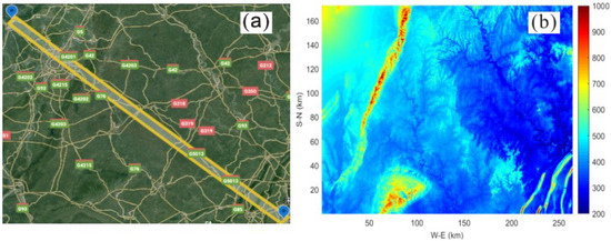
Figure 6.
The calculation area in the PE model and its topographic map with elevation: (a) beam-covered area. (b) The elevation distribution.
The surface medium model can be obtained by classifying and processing the color satellite maps. Using color to distinguish different ground attachments and combined with the elevation information, different ground attachments with the same or similar colors can be distinguished. The color map where the calculation area is located can be divided into five categories: wet soil, freshwater, concrete (buildings), forests, and grass. Their electromagnetic parameters are given in Table 1.

Table 1.
Electromagnetic parameters of different media.
Based on the color classification, a surface medium database for PE is established. Substituting the average refractivity N and the modified refractivity M of the two cities into the PE method with the actual terrain model, the propagation properties of the radio wave in the troposphere in the area designated in Figure 6a can be simulated.
4.3. Calculation Results
In the PE model, we set n = 1 at first (atmospheric refraction is not considered); thus, the calculation results only reflect the influence of the terrain of the calculation space shown in Figure 6a. Electric field distribution dBV/m at the center of the calculation space shown in Figure 6a (the longitudinal section where the transmitting and receiving antennas are located) is shown in Figure 7a. The bottom without the electric field is the terrain profile. In order to reduce calculation time, the height is set at 1200 m.
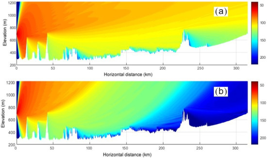
Figure 7.
Electric field distribution calculated by PE model: (a) Without refraction. (b) With modified refractivity.
The scattering from the ground can be observed in Figure 7a. Because the propagation medium is uniform (n = 1), the radio wave propagates along a straight line [29]. ( is the electric field intensity at the receiving antenna, and is the normalized electric field intensity at the transmitting antenna.) The attenuation of the electric field, which is defined as [18] in this condition, is 143.1 dB.
Using the modified refractive index (11) into the PE model, the effect of the curvature of the Earth can be considered. The calculated electric-field distribution is illustrated in Figure 7b, with an electric field attenuation of 223.4 dB.
Figure 8 shows the calculation results of the entire troposphere of the calculation space. The attenuation of the electric field in the receiving antenna is 223.5 dB. The result is the same when the calculated height is 1200 m; however, the calculation time increases almost eight times (with the same computer, the calculation time increased from 0.45 h to 4 h). However, the latter gives detailed propagation characteristics of the radio wave in the entire troposphere.
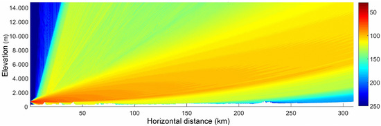
Figure 8.
The electric field distribution in the longitudinal section of the entire troposphere in the calculation space with modified refractivity.
4.4. Effect of Antenna Elevation Angle
As mentioned before, the elevation angle of the transmitting and receiving antennas is 0, but when the curvature of the Earth is taken into account, the elevation angle becomes . The resultant electric field distribution is illustrated in Figure 9, with a corresponding electric field attenuation of 232.0 dB. The electric field attenuation as a function of the elevation angle is shown in Figure 10. It can be observed in Figure 10 that the increase in the elevation angle of the transmitting antenna will increase the attenuation of the electric field, while the attenuation of the electric field decreases first and then increases as the elevation angle of the receiving antenna increases.
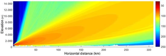
Figure 9.
The electric field distribution when the elevation angle of transmitting antenna is .
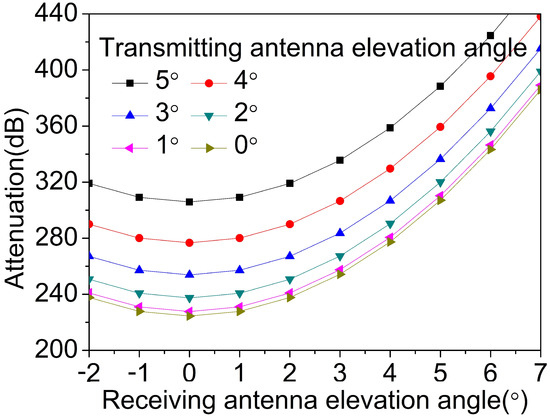
Figure 10.
Changes in attenuation caused by changes in antenna elevation angle.
5. Comparison of Results
5.1. The Propagation Paths
As Figure 7, Figure 8 and Figure 9 show, the PE model gives a picture of the propagation path of radio waves in the troposphere. Since the PE model takes into account not only the atmospheric refraction but also the effects of terrain, comparing the radio wave propagation path obtained by the PE model with the numerical method proposed in Section 3 can acquire more useful details.
As Figure 5 shows, after the curvature of the Earth is taken into account, the propagation path of radio waves bends upwards [28]. Actually, the elevation angle of the transmitting antenna given in Figure 9 is . Because the beam angle of the transmitting antenna is set as , the elevation angles of the upper and lower edges of the radio waves emitted by the antenna are and , which can be obtained from Figure 11a.
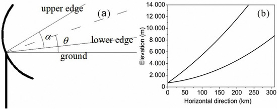
Figure 11.
Elevation angles and propagation paths: (a) Relation between transmitting antenna beam angle and elevation angle. (b) Radio wave propagation paths at different elevation angles.
Utilizing the modified refractive index M, Figure 11b shows the propagation paths of the upper and lower edges of the radio wave emitted by the antenna with elevation angles of and calculated by the numerical method proposed in Section 4. Figure 12 provides a comparison of propagation paths obtained by the two models.
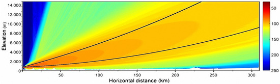
Figure 12.
Comparison of propagation paths obtained by the path tracing numerical model and the PE model.
The results shown in Figure 11b only considered the effect of atmospheric refraction, whereas the propagation image obtained by the PE model in Figure 10 also considers the influence of the terrain; thus, the propagation paths obtained by the two models are different. However, we observe in Figure 12 that the main energy of the radio wave is still concentrated within the upper and lower edges shown in Figure 11b.
5.2. The PE Method and the Measured Data
Measurements have been conducted by The Science and Technology on Electronic Information Control Laboratory in 2020. The calculation condition is provided in this sections. These include the transmitting and receiving antenna parameters, location, elevation, and the normalized source. Table 2 gives four groups of received electric field attenuation values. These values are chosen from 1-year data and represent the results during four seasons.
Table 2.
The measured attenuation of the electric field (dB) in different seasons (the elevation angles of the transmitting and receiving antennas are kept at ).
6. Conclusions
The propagation characteristics of radio waves in the troposphere have been modeled by a numerical method and PE. The numerical method can be utilized to quickly track the propagation path of radio waves. Combining the PE method with the terrain model, the propagation and attenuation image of radio waves in the troposphere can be obtained.
Using the PE model, we observed that an increase in the elevation angle of the transmitting antenna results in an increase in the attenuation of the electric field. When the elevation angle of the receiving antenna is less than 0, the attenuation of the electric field decreases as the elevation angle increases, but when the elevation angle of the receiving antenna is greater than 0, the attenuation of the electric field increases as the elevation angle increases.
The effects of the curvature of the Earth can be demonstrated by using the modified refractive index in the numerical model and the PE model. After taking into account the curvature of the Earth, the propagation path of a radio wave is found to bend upwards. The propagation paths obtained by the numerical method and the PE model were found to be approximately identical.
Author Contributions
Conceptualization, M.X. and T.T.; methodology, O.M.R. and M.O.; software, T.T.; data curation, M.X. and Z.J.; writing—original draft preparation, M.O.; writing—review and editing, M.A. and M.Z. All authors have read and agreed to the published version of the manuscript.
Funding
This research was funded by the Science and Technology on Electronic Information Control Laboratory.
Institutional Review Board Statement
Not applicable.
Informed Consent Statement
Not applicable.
Data Availability Statement
Not applicable.
Conflicts of Interest
The authors declare no conflict of interest.
References
- Yang, Y.; Long, Y. Modeling EM pulse propagation in the troposphere based on the TDPE method. IEEE Antennas Wirel. Propag. Lett. 2013, 12, 190–193. [Google Scholar] [CrossRef]
- Zelley, A.C.; Constantinou, C.C. A three-dimensional parabolic equation applied to VHF/UHF propagation over irregular terrain. IEEE Trans. Antennas Propag. 1999, 47, 1586–1596. [Google Scholar] [CrossRef]
- Holm, P.; Lundborg, B.; Waern, A. Parabolic Equation Technique in Vegetation and Urban Environments; FOI Report; Swedish Defence Research Agency: Linköping, Sweden, 2003. [Google Scholar]
- Awadallah, R.S.; Gehman, J.Z.; Kuttler, J.R.; Newkirk, M.H. Effects of lateral terrain variations on tropospheric radar propagation. IEEE Trans. Antennas Propag. 2005, 53, 420–434. [Google Scholar] [CrossRef]
- Ozgun, O. Recursive two-way parabolic equation approach for modeling terrain effects in tropospheric propagation. IEEE Trans. Antennas Propag. 2005, 57, 2706–2714. [Google Scholar] [CrossRef]
- Sizun, H.; de Fornel, P. Radio Wave Propagation for Telecommunication Applications; Springer: Paris, France, 2005; p. 171. [Google Scholar]
- Sofos, T.; Constantinou, P. Propagation model for vegetation effects in terrestrial and satellite mobile systems. IEEE Trans. Antennas Propag. 2004, 52, 1917–1920. [Google Scholar] [CrossRef]
- Arshad, K.; Katsriku, F.; Lasebae, A. Radiowave VHF Propagation modelling in forest using finite elements. In Proceedings of the 2006 2nd International Conference on Information & Communication Technologies, Damascus, Syria, 24–28 April 2006; Volume 2, pp. 2146–2149. [Google Scholar]
- Gay-Fernandez, J.A.; Cuinas, I. Peer to peer wireless propagation measurements and path-loss modeling in vegetated environments. IEEE Trans. Antennas Propag. 2013, 61, 3302–3311. [Google Scholar] [CrossRef]
- Bai, R.; Liao, C.; Sheng, N.; Zhang, Q. Prediction of wave propagation over digital terrain by parabolic equation model. In Proceedings of the 2013 5th IEEE International Symposium on Microwave, Antenna, Propagation and EMC Technologies for Wireless Communications, Chengdu, China, 29–31 October 2013; pp. 458–461. [Google Scholar]
- Guan, X.-W.; Guo, L.-X.; Wang, Y.-J.; Li, Q.-L. Parabolic Equation Modeling of Propagation over Terrain Using Digital Elevation Model. Int. J. Antennas Propag. 2018, 2018, 1–6. [Google Scholar] [CrossRef] [Green Version]
- Goudar, B.; Watson, R.J. Variability in propagation path delay for atmospheric remote sensing. In Proceedings of the 2014 IEEE Geoscience and Remote Sensing Symposium, Quebec City, QC, Canada, 13–18 July 2014; pp. 4127–4130. [Google Scholar]
- Levis, C.; Johnson, J.T.; Teixeira, F.L. Radiowave Propagation: Physics and Applications; John Wiley & Sons: Hoboken, NJ, USA, 2010; pp. 120–134. [Google Scholar]
- Tao, T.; Guo, L.; Liu, L. Numerical modeling the propagation path of radio waves with atmospheric refractivity. Microw. Opt. Technol. Lett. 2020, 62, 1651–1655. [Google Scholar]
- Liu, Y.; Tang, T.; Liu, G.; Olaimat, M. Error Analysis of the Numerical Method for Correcting the Propagation of EM waves in the Troposphere. J. Microw. Optoelectron. Electromagn. Appl. 2020, 19, 407–414. [Google Scholar] [CrossRef]
- Arshad, K.; Katsriku, F.; Lasebae, A. Propagation modelling in troposphere using paraxial form of Helmholtz equation. In Proceedings of the 2005 Asia-Pacific Microwave Conference Proceedings, Suzhou, China, 4–7 December 2005; pp. 752–755. [Google Scholar]
- Fang, J.; Li, Q. Simulation method for wave propagation in the troposphere duct. In Proceedings of the 6th International Symposium on Antennas, Propagation and EM Theory, Beijing, China, 28 October–1 November 2003; pp. 524–527. [Google Scholar]
- Kang, S.; Wang, H. Analysis of microwave over-the-horizon propagation on the sea. In Proceedings of the 2009 Asia Pacific Microwave Conference, Singapore, 7–10 December 2009; pp. 1545–1548. [Google Scholar]
- Ozgun, Z.; Tanyer, S.G.; Erol, C.B. An examination of the Fourier split-step method of representing electromagnetic propagation in the troposphere. In Proceedings of the IEEE International Geoscience and Remote Sensing Symposium, Honolulu, HI, USA, 25–30 July 2010; Volume 6, pp. 3548–3550. [Google Scholar]
- Sirkova, I.; Mikhalev, M. Parabolic wave equation method applied to the tropospheric ducting propagation problem: A survey. Electromagnetics 2006, 26, 155–173. [Google Scholar] [CrossRef]
- Sirkova, I. Brief review on PE method application to propagation channel modeling in sea environment. Open Eng. 2011, 2, 19–38. [Google Scholar] [CrossRef]
- Karagianni, E.A.; Mitropoulos, A.P.; Latif, I.; Kavousanos-Kavousanakis, A.; Koukos, J.; Fafalios, M.E. Atmospheric effects on em propagation and weather effects on the performance of a dual band antenna for wlan communications. Nausivios Chora 2014 Part B Electr. Eng. Comput. Sci. 2014, 5, B-29. [Google Scholar]
- Zhao, X. On enhancement effect of scattering communication by acoustic wave interference in the troposphere. In Proceedings of the 2016 Progress in Electromagnetic Research Symposium, Shanghai, China, 8–11 August 2016; pp. 3634–3637. [Google Scholar]
- Abdullah, M.; Ullah, H.E.; Rasheed, H.; Mufti, N. An investigation of the radio refractive conditions in lowest portions of the troposphere near Margalla Hills, Pakistan. In Proceedings of the 2016 IEEE-APS Topical Conference on Antennas and Propagation in Wireless Communications, Cairns, QLD, Australia, 19–23 September 2016; pp. 225–228. [Google Scholar]
- Ning, W.; Li-xin, G.; Zhen-wei, Z.; Le-ke, L.; Zong-hua, D. Retrieving the troposphere duct by using ground-based radiometric profiler in South Coast in China. In Proceedings of the 2016 11th International Symposium on Antennas, Propagation and EM Theory, Guilin, China, 18–21 October 2016; pp. 216–219. [Google Scholar]
- University of Wyoming, Department of Atmospheric Science, Soundings. Available online: http://weather.uwyo.edu/upperair/sounding.html (accessed on 10 December 2021).
- Grabner, M.; Kvicera, V.A. Electromagnetic Waves; InTech: Rijeka, Croatia, 2011; pp. 139–156. [Google Scholar]
- Chao, Y.; Li-Xin, G.; Hong-Qiang, L. Modelling the Radio Wave Propagation in the Troposphere with Discrete Mixed Fourier Method. In Proceedings of the 2008 8th International Symposium on Antennas, Propagation and EM Theory, Kunming, China, 2–5 November2008; pp. 389–392. [Google Scholar]
- Zhang, D.; Liao, C.; Feng, J.; Deng, X. Pulse-Compression Signal Propagation and Parameter Estimation in the Troposphere With Parabolic Equation. IEEE Access 2019, 7, 99917–99927. [Google Scholar] [CrossRef]
Publisher’s Note: MDPI stays neutral with regard to jurisdictional claims in published maps and institutional affiliations. |
© 2022 by the authors. Licensee MDPI, Basel, Switzerland. This article is an open access article distributed under the terms and conditions of the Creative Commons Attribution (CC BY) license (https://creativecommons.org/licenses/by/4.0/).