Fast Dual-LiDAR Reconstruction for Dynamic Wind Field Retrieval

Abstract

With the advantages of high accuracy, high spatial resolution, and long measurement range, LiDAR is considered as the most suitable measurement technique to deliver quantitative imaging of wind fields. However, for complex wind fields, such as monitoring wind turbine wakes where both the temporal resolution and reconstruction speed are of great significance, the conventional LiDAR system lacks the temporal resolution to capture the fast changes of wind turbine wake fields. In this paper, a novel dynamic wind retrieval method is developed to improve temporal resolution using the unsynchronised dual-LiDAR scanning scheme. By exploiting the temporal redundancy information of the LiDAR Line-of-Sight (LoS) data in successive frames, a reduced number of LiDAR scanning points is required for the 2D horizontal wind field retrieval with the help of unsynchronised dual-LiDAR wind scanning scheme, low-rank data up-sampling and a divergence-free regularised wind retrieval algorithm. Numerical simulation is performed to validate the proposed method. Results show that the temporal resolution of LiDAR wind retrieval can be improved by a factor of 2 to 8 and provide acceptable results with good spatial resolution.

1. Introduction

As a result of an increasing demand for renewable wind energy, modern wind turbines and large-scale wind farms are being developed at a rapid rate. Due to the space limitation for wind farms, wind turbines are implemented into dense clusters [1] so that the efficiency of the wind turbines are affected by the turbine wake flows, which reduces the energy production and increases the probability of fatigue on the turbine components [2,3]. To address this problem, accurate and fast monitoring of the wind field is a key point to provide essential data for wind farm layout, real-time control and maintenance [4]. One of the most promising techniques for imaging wind fields is the Doppler light detection and ranging (LiDAR). Compared to other techniques, LiDAR has the advantages of high accuracy, high spatial resolution, and long measurement range [5], which makes it the most suitable measurement technique to image turbine wakes in wind fields [6].

Wind LiDAR can only measure the radial velocity in the direction of the laser beams but ignores the wind component transversal to the laser beams. Therefore, a single LiDAR system cannot provide sufficient data to fully retrieve a 2D/3D wind field [7,8]. A common practice of industrial application assumes flow homogeneity, which is not suitable for turbine wake wind field imaging due to complex wind conditions [9,10]. Cherukuru developed a 2D VAR wind retrieval method [9]. Using radial velocity advection equation as an additional constraint, the proposed method was able to retrieve a 2D wind field from measurements based on a single LiDAR. However, this method lacks accuracy due to the complexity of wind fields and the low signal-to-noise ratio (SNR) of LiDAR measurements [11].

To overcome this problem, a research group at the Technical University of Denmark (DTU) investigated multiple LiDAR system, which utilised spatially coordinated and temporally synchronised Doppler LiDAR units to scan over the same area from different locations and retrieve wind images from three radial velocities [12,13]. Specifically, when dual-LiDAR observations were used in 2D VAR retrievals, the accuracy largely increased compared to the single LiDAR system [14]. However, the high-quality wind retrieval of multiple LiDAR systems is at the cost of high equipment and operation cost [15].

Alternatively, van Dooren proposed a Multiple-LiDAR Wind Field Evaluation Algorithm (MuLiWEA) [7]. With the help of grid interpolation, the proposed wind retrieval method did not require a set of fully synchronised dual-LiDAR measurements. The two LiDAR systems can scan the sensing area individually without synchronisation of LiDAR beams for intersecting points’ radial velocity measurement [7]. Hon from Hong Kong Observatory presented a fast dual-Doppler LiDAR retrieval method, which utilised data from two unsynchronised LiDAR systems to scan the boundary layer wind profile over Hong Kong International Airport. This algorithm offers the possibility to use measurements from scanning scenarios with low complexity and fast area coverage. However, this method also requires the frozen field assumption that the wind field remains constant during the whole LiDAR scanning process, which may not be suitable for the fast-changing turbine wake wind field.

The unsynchronised LiDAR system also offers the flexibility for spatial and temporal resolution adjustment [16]. Unlike the synchronised dual-LiDAR system, whose scanning trajectories are predesigned for intersecting points in the sensing area, the unsynchronised LiDAR system can easily change the scanning pattern and interval for optimised spatial-temporal resolution. Beck studied the dual-LiDAR spatial-temporal conversion method for LiDAR measurement up-sampling, which increased the temporal resolution of the LiDAR data by a factor of 2.4 to 40 [17].

Despite the improvement in temporal resolution, Beck’s up-sampling method is computationally expensive. During the spatial-temporal conversion, the interpolation is computed based on the temporal evolution of wind field in a point-wise and iterative fashion, which is time consuming and memory intensive [17]. After each interpolation, wind velocities on the regular cartesian grids are displaced to an irregular grid. A post interpolation process is needed, which maps the wind velocities onto the initial grid using natural-neighbour interpolation. Consequently, this will not only cause additional computational cost, but also cause shift error within the retrieved wind velocity.

In order to improve the temporal resolution of LiDAR wind retrieval and capture the dynamic characteristics of the fast-changing turbine wake wind field, in this study, a novel approach is proposed to reduce the number of LiDAR scans for fast wind field imaging using dual-LiDAR system. There are two research objectives to be achieved: (1) To improve the temporal resolution of wind retrievals to catch fast wind field changes; (2) to quantitatively assure the spatial resolution of wind images for revealing the detailed wind field. To achieve the proposed objectives, the following steps are implemented: (1) Obtain Line of Sight (LoS) data from an unsynchronised dual-LiDAR system and align the two LoS dataset into pre-set grids, then apply matrix completion for LoS data up-sampling; (2) design spatial regularisation for 2D horizontal wind field, then apply a robust reconstruction algorithm for wind retrieval. The novelties of the proposed method are to use low-rank matrix completion for LoS data up-sampling and build a spatial regularisation with vector Laplacian and divergence-free term for better wind retrieval quality. Compared to other LiDAR up-sampling strategies, such as Beck’s method, the proposed method does not require the calculation of wind field evolution and a post interpolation process, therefore it has the advantages of high flexibility in up-sampling factors and reduction in computational cost due to the fast LoS data matrix completion process. A simulation study is carried out to validate the performance of the proposed method.

2. Methods

2.1. Forward Modelling of LiDAR

The forward problem of LiDAR wind retrieval defines the relationship between the Line-of-Sight (LoS) radial velocity v_r and wind speed components u, v, and w in x-, y- and z-direction. In this paper, the vertical wind speed component w is ignored because the elevation angles φ of the PPI scans applied are commonly small, and, therefore, only horizontal wind velocity components u, and v are considered. Therefore, the radial velocity $v_r$ is defined as [18]:

$$v_r=u\cos (\phi )\cos (\theta )+v\cos (\phi )\sin (\theta )$$

(1)

where θ is the azimuth angle.

In addition, the flow is discretised into N square grids with side length of d, which is the spatial resolution of LiDAR wind retrieval. Given the scanning trajectory, the forward model is defined in matrix form as:

$$v_r=APu+BPv$$

(2)

where ${\mathit{v}}_{\mathit{r}}\in {ℝ}^{M\times \mathbf{1}}$ is the radial velocity and M denotes the number of scanning points, $\mathit{u}\in {ℝ}^{N\times \mathit{1}}$ and $\mathit{v}\in {ℝ}^{N\times \mathit{1}}$ are the discretised wind speed components and $\mathit{P}\in {ℝ}^{M\times \mathit{N}}$ is the selection matrix built according to the LiDAR scanning points, which is defined as:

$$P_{i,j}=\left\{\begin{array}{c}1\hspace{1em}\hspace{1em}\hspace{1em}if sca{n}_j in pixe{l}_{\mathrm{i}}\hfill \\ 0\hspace{1em}\hspace{1em}\hspace{1em}\hspace{1em}\hspace{1em}else\hfill \end{array}\right.$$

(3)

where $\mathit{A}\in {ℝ}^{M\times M}$ and $\mathit{B}\in {ℝ}^{M\times M}$ are the measurement matrices that transform the wind velocity components to the radial velocity, whose elements are defined as:

$$\begin{array}{c}{A}_i=\cos ({\phi }_i)\sin ({\theta }_i)\\ B_i=\cos ({\phi }_i)\cos ({\theta }_i)\end{array}$$

(4)

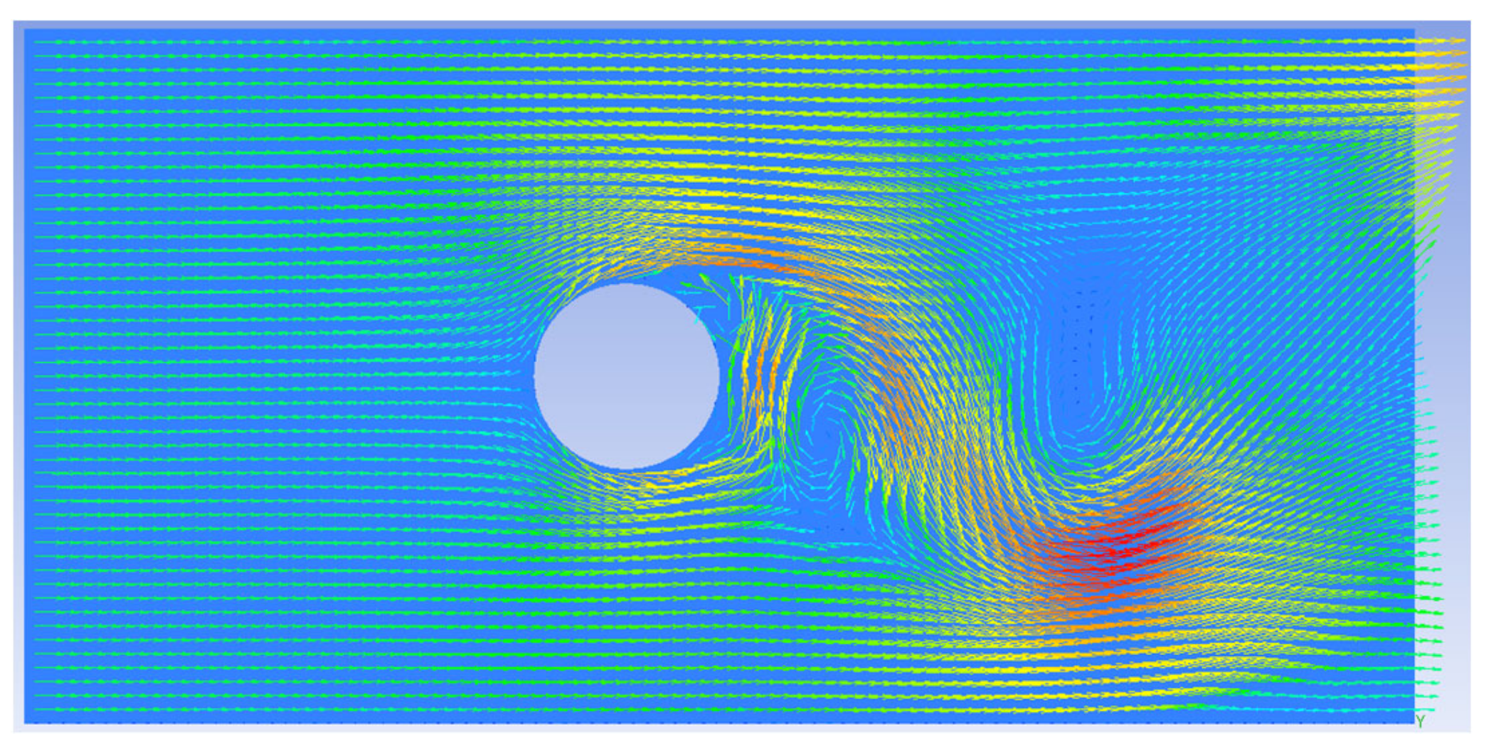
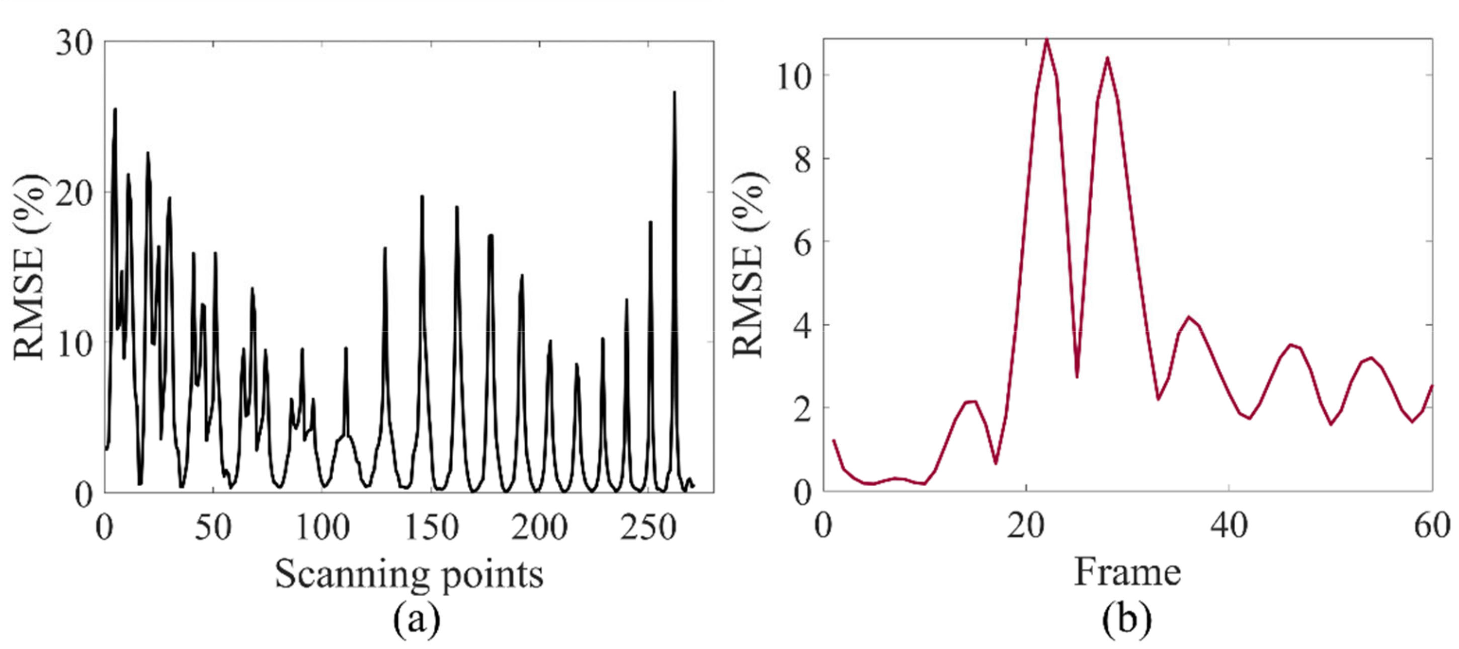
The forward model defined above is based on the frozen field assumption that the wind field remains constant during the whole LiDAR scanning process, without considering the dynamic flow characteristic when the M number of scanning points are collected. As a result, the retrieved wind field will be dominated by the retrieval error and the wind velocity changes cannot be resolved. An example is shown in Figure 1.

Differently, in this paper, the wind velocity is considered to be stationary for a short time period t, which is the temporal resolution of the target LiDAR wind retrieval. Therefore, the dynamic forward problem can be modified. Specifically, the radial velocities and wind velocity for each time interval can be stacked as columns and denoted as ${\mathit{V}}_{\mathit{r}}=\left[{\mathit{v}}_{r,1},{\mathit{v}}_{r,2},\dots ,{\mathit{v}}_{r,T}\right]$, $\mathit{V}=\left[{\mathit{v}}_1,{\mathit{v}}_2,\dots ,{\mathit{v}}_T\right]$ and $\mathit{U}=\left[{\mathit{u}}_1,{\mathit{u}}_2,\dots ,{\mathit{u}}_T\right]$, where T is the number of time intervals, and ${\mathit{v}}_{r,1}\in {ℝ}^{M\times \mathbf{1}}$ is the radial velocities measured within each time interval.

Each column refers to one time interval. Then, the forward problem for successive LiDAR measurements can be written as:

$$V_r=AU+BV$$

(5)

where the block diagonal matrices are given as $\mathit{A}=diag\left({\mathit{A}}_1{\mathit{P}}_1,{\mathit{A}}_2{\mathit{P}}_2,\dots ,{\mathit{A}}_T{\mathit{P}}_T\right)$ and $\mathit{B}=diag\left({\mathit{B}}_1{\mathit{P}}_1,{\mathit{B}}_2{\mathit{P}}_2,\dots ,{\mathit{B}}_T{\mathit{P}}_T\right)$.

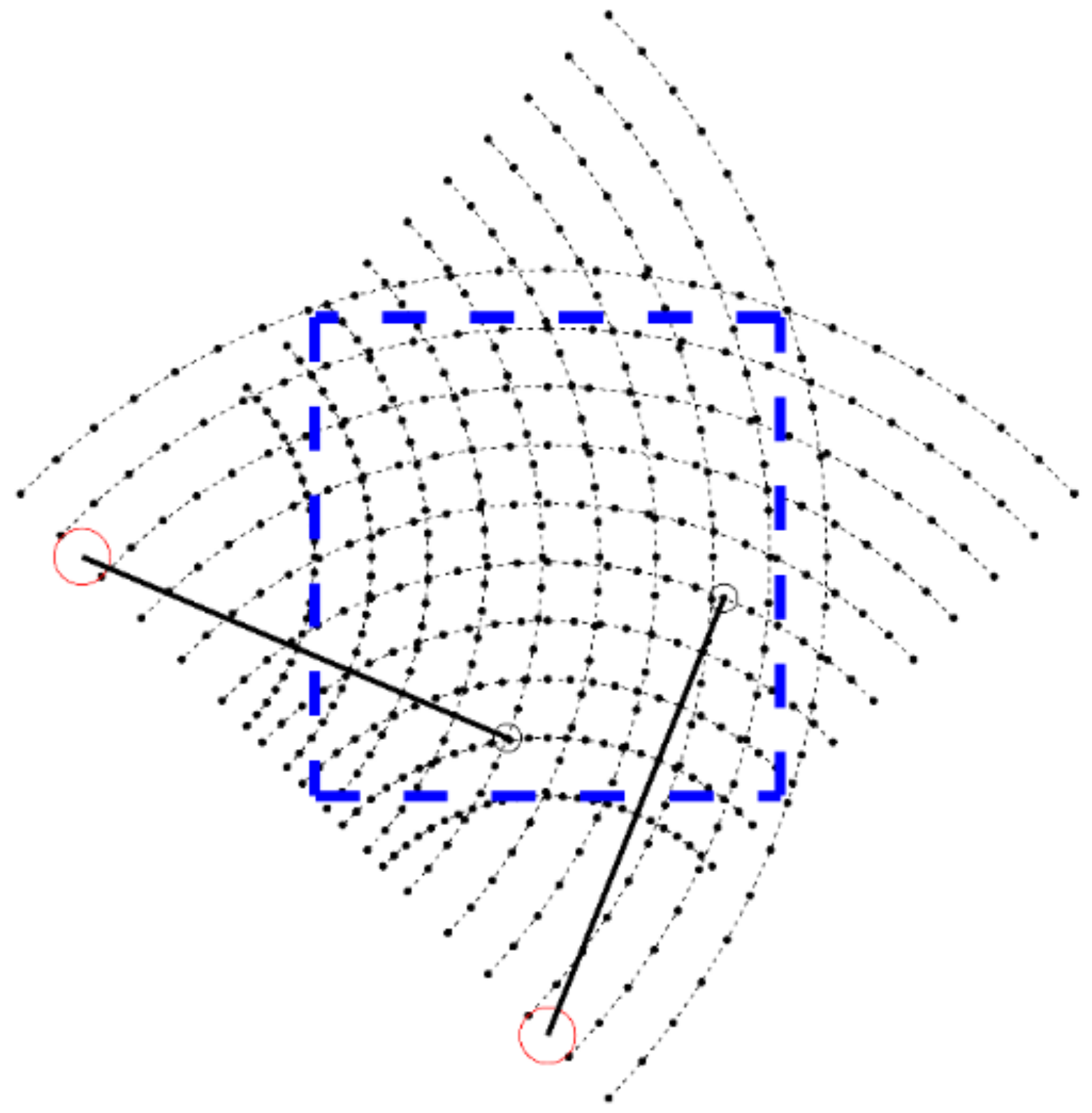
2.2. Dual-LiDAR Wind Retrieval

To resolve the 2D horizontal wind field, a dual-LiDAR system is applied. Inspired by van Dooren’s research [7], the two LiDARs work in a unsynchronised way, that performs PPI scans independently to cover the sensing area, as shown in Figure 2.

Radial velocities from the dual-LiDAR system can be used to reconstruct the 2D wind field by solving the following inverse problem:

$$\underset{U,V}{\min }{‖V_{r,1}-A_{1}U-B_{1}V‖}_2^2+{‖V_{r,2}-A_{2}U-B_{2}V‖}_2^2+R\mathbf{(}U,V\mathbf{)}$$

(6)

where R(U,V) denotes the regularisation term, which consists of the divergence-free regularisation and the Tikhonov regularisation.

Firstly, the 2D horizontal wind velocity field can be considered as a divergence-free vector field. This assumption is valid, as the stratification in the atmosphere caused by gravity makes the horizontal velocity u and v greater than the vertical velocity w by a factor of 10–100 [19]. Usually for the wind data used here, w can be ignored, and (u,v) becomes a divergence-free vector field [19]. Therefore, we can apply a divergence-free constraint in the reconstruction of wind velocity field.

Secondly, vector Laplacian regularisation is applied to pose a smoothness constraint to the wind components in x- and y-axis, respectively, which stabilises the retrieval process when the inverse problem is solved.

Generally, the R(U,V) is defined as [20]:

$$R(U,V)={\alpha }_1{‖\nabla ·(U,V)‖}_1+{\alpha }_2{‖{\nabla }^2(U,V)‖}_2^2$$

(7)

where α₁ and α₂ are the regularisation parameters for each regularisation term. The regularisation parameters are determined empirically based on the simulation results and kept constant when solving the inverse problem of wind retrieval, given all the different datasets [1,2]. The vector divergence term and vector Laplacian can be determined by the following equations.

$$\nabla \cdot (U,V)={\displaystyle \sum _{t=1}^T\nabla \cdot (u_t,v_t)}={\displaystyle \sum _{t=1}^T{D}_x{u}_t+D_{\mathrm{y}}{v}_t}$$

(8)

$$\begin{array}{c}{\nabla }^2(U,V)={\displaystyle \sum _{t=1}^T{\nabla }^2(u_t,v_t)}={\displaystyle \sum _{t=1}^T\left(\frac{{\partial }^2{u}_t}{\partial x^2}+\frac{{\partial }^2{u}_t}{\partial y^2}+\frac{{\partial }^2{v}_t}{\partial x^2}+\frac{{\partial }^2{v}_t}{\partial y^2}\right)}\\ \hspace{1em}\hspace{1em}={\displaystyle \sum _{t=1}^T\left((D_x{D}_x+D_y{D}_y)u_t+(D_x{D}_x+D_y{D}_y)v_t\right)}\end{array}$$

(9)

where ${\mathit{D}}_{\mathit{x}},{\mathit{D}}_{\mathit{y}}\in {ℝ}^{N\times N}$ are the two directional discrete operators along x- and y-axis for the calculation of the vector divergence and Laplacian, which is defined as a finite differential approximation. The discrete 2nd order finite differential approximation is used inside the sensing area and 1st order differential for boundary pixel.

$${\nabla }_{i,j}^x\cdot v=\left\{\begin{array}{c}\frac{v_x(i-1,j)+v_x(i+1,j)-2v_x(i,j)}{2d}\\ \frac{v_x(i-1,j)-v_x(i,j)}{d}\\ \frac{v_x(i+1,j)-v_x(i,j)}{d}\end{array}\begin{array}{c}\mathrm{left}\mathrm{boundary}\\ \mathrm{right}\mathrm{boundary}\end{array}\right.$$

(10)

Consequently, u and v in Equation (10) can be solved jointly and efficiently using the interior-point method [21], which is implemented by the MOSEK optimisation suite in MATLAB [22].

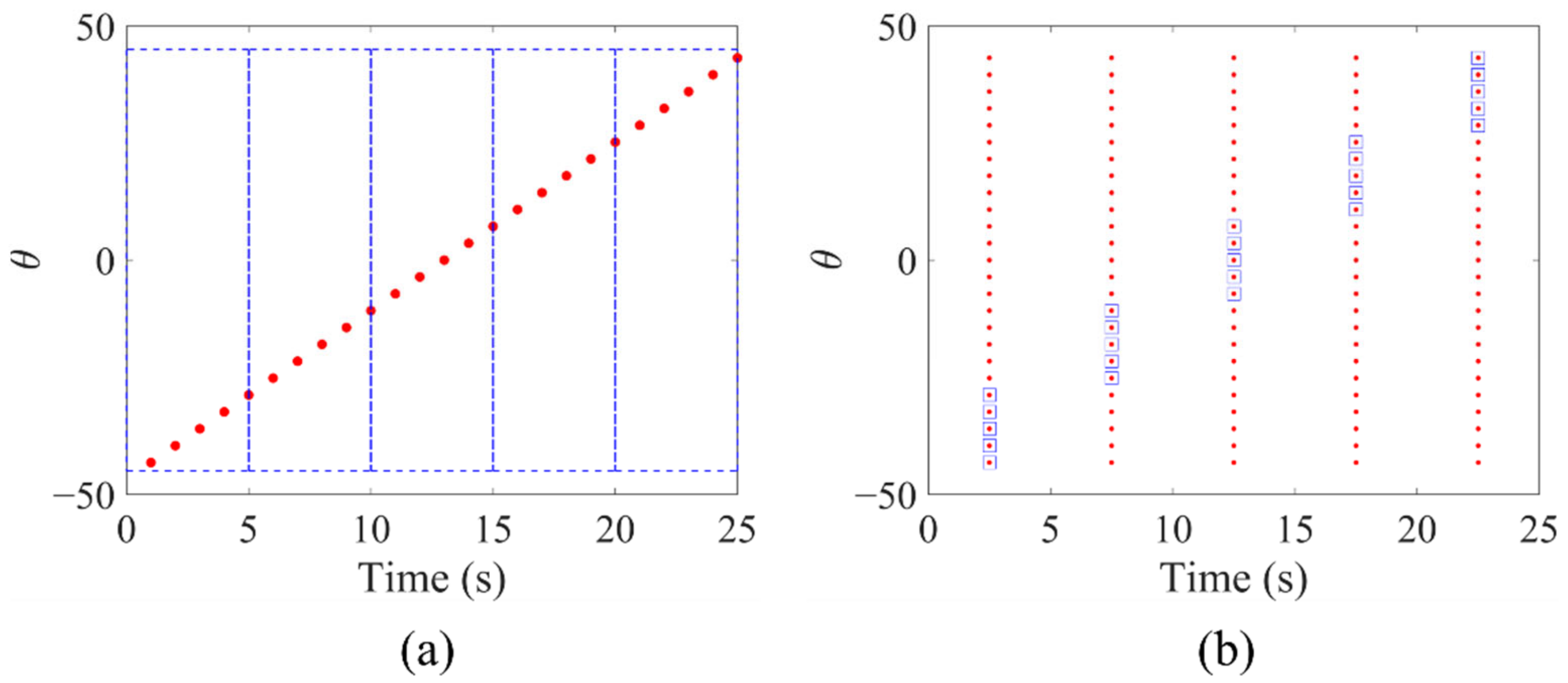
2.3. Spatial-Temporal Conversion and Up-Sampling

The temporal resolution of LiDAR wind retrieval is determined by the length of the measurement time window, which should be chosen based on the time scale of the wind field evolving. Therefore, for the fast-changing turbine wake wind field, the short time window allows a reduced number of LiDAR scans. As shown in Figure 3, within each time interval, only a small number of radial velocities can be obtained. Due to the missing scanning points, the retrieved accuracy of the wind field for each time step is greatly affected. To solve this problem, Beck proposed a temporal up-sampling method using spatial-temporal conversion. However, their method relies on the backwards-oriented propagation, which is computational expensive during the calculation of wind field evolution. Differently, in this paper, we present a temporal up-sampling method for LiDAR dataset based on the classic matrix completion algorithm. The general idea is to calculate the missing scanning data within each time step based on the spatial and temporal correlations of the radial velocity, as shown in Figure 3b. Our target is to maintain quantitative accuracy during the data interpolation, without spending too many computational resources on calculating wind flow propagation.

To illustrate the up-sampling method, we only consider a simple case when a reconstructed wind field uses single the LiDAR dataset, but it is straightforward to extend the proposed method for the dual-LiDAR system.

To begin with, LiDAR dataset is a K by T radial velocity matrix V_r containing a total of M radial velocity measurements. To reconstruct the dynamic wind field with T time steps, the fully sampled M by T radial velocity matrix $\mathit{V}{\mathit{F}}_{\mathit{r}}=\left[\mathit{v}{\mathit{f}}_{r,1},\mathit{v}{\mathit{f}}_{r,2},\dots ,\mathit{v}{\mathit{f}}_{r,T}\right]$ is needed. Therefore, the problem is to calculate the M by T fully sampled data, given a K by T subset V_r.

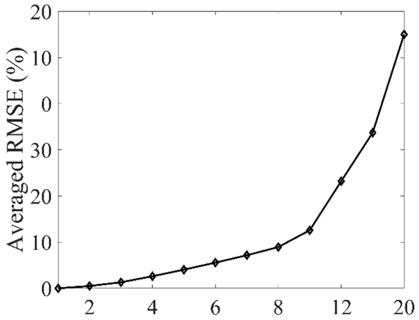
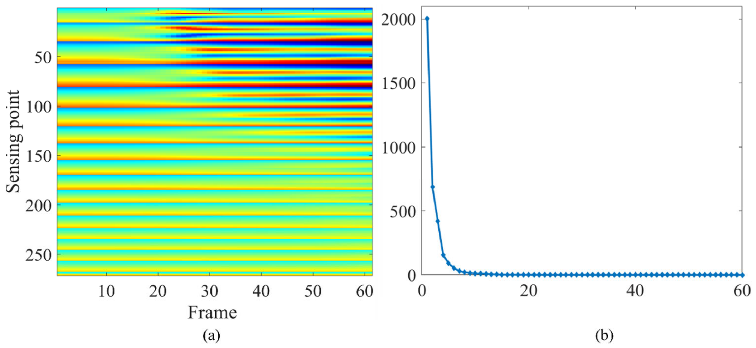
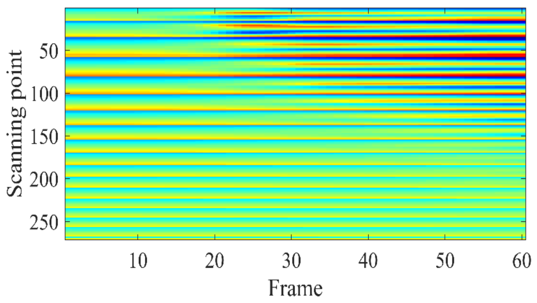
The key to matrix completion is to exploit the correlations of the radial velocities in the spatial and temporal domain. Figure 4a shows the fully sampled radial velocity map calculated from 60 successive frames of wind field. The corresponding singular values are shown in Figure 4b, which shows that the fully sampled radial velocity matrix is rank deficient. Therefore, low-rank prior can be applied here for matrix completion, which solves the following problem as:

$$\begin{array}{l}\underset{VF}{\min }{‖VF‖}_{*}\\ s.t.VF(i,j)=v_r(i,j)\forall i,j\in scanning\end{array}$$

(11)

The classic Riemannian Optimisation [23] method is used to solve Equation (11).

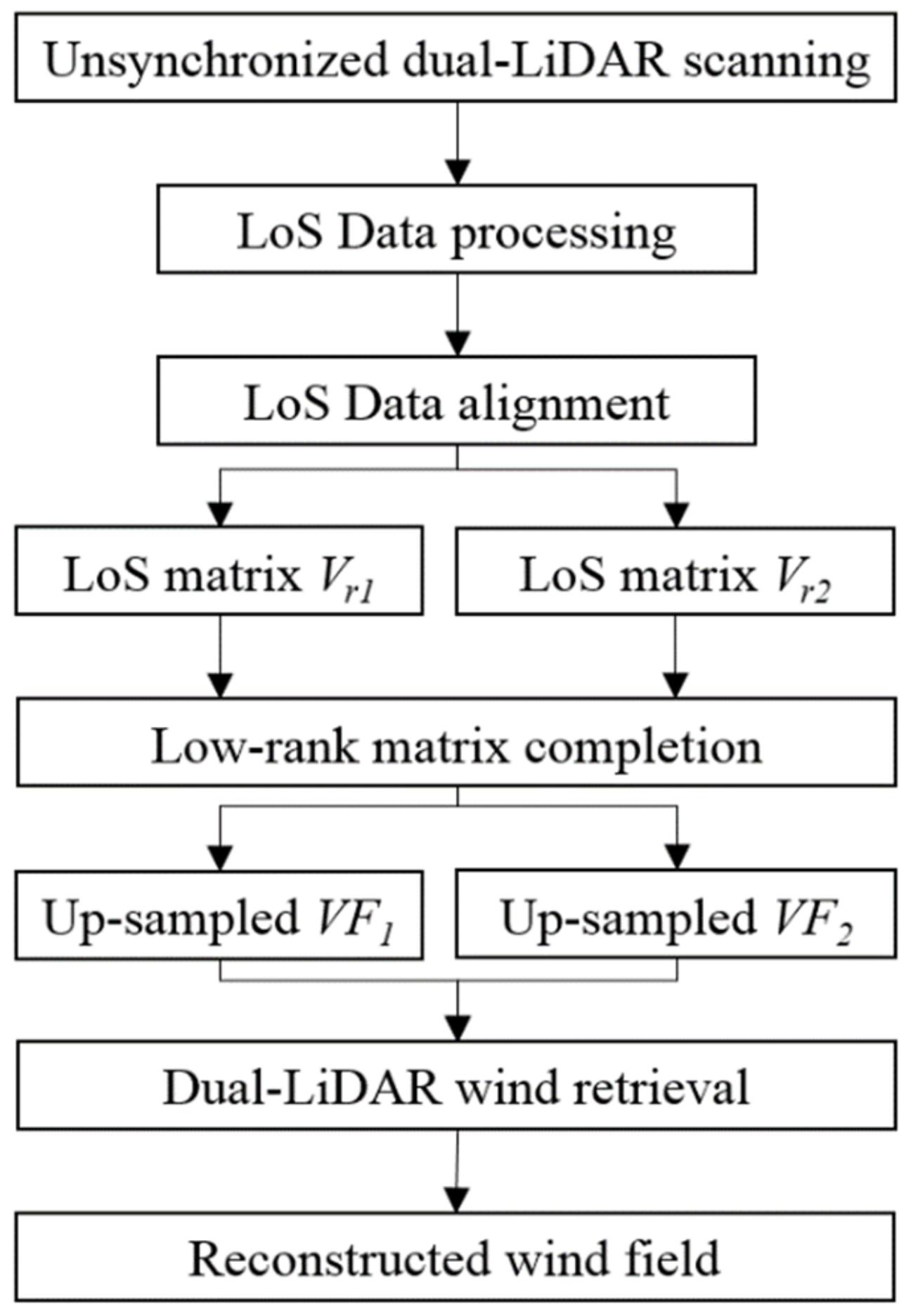
2.4. Summary of the Time-Resolved Dual-LiDAR Imaging

The flow chart of the time-resolved dual-LiDAR imaging system is shown in Figure 5, and details of the flowchart are listed as follows:

• The data collection step of the time-resolved dual-LiDAR imaging system. The region of interest is covered by the two PPI scans using the dual-LiDAR system. Then, the corresponding LoS data are collected;
• Align the two LoS datasets into different time slots and scanning position to form two LoS velocity matrices $V_r$ with missing entities. Then, low-rank matrix completion is conducted to fill the missing entities in the V_r matrix;
• Perform wind field retrieval from the up-sampled datasets based on the divergence-free regularised reconstruction algorithm.

Figure 5. The flowchart of the time-resolved dual-LiDAR imaging system.

Figure 5. The flowchart of the time-resolved dual-LiDAR imaging system.

3. Results

3.1. Simulation Setup

In this section, the performance of the proposed method is evaluated with a series of numerical simulations, including the simulation for the 2D horizontal wind fields of turbine wake, the forward modelling which calculates the LoS data from the wind fields, and the wind retrieval based on the two unsynchronised LoS data.

For the simulation of turbine wake wind field, we consider a rectangular area with length and width of 60 m and 30 m, respectively. The wind turbine pile is represented by a circle with diameter of 4 m, located in the centre of a 26 m by 5 m rectangular area. The 2D horizontal wind field of the turbine wake is simulated in the Fluent. The region of interest is discretised with triangular mesh, using 25,594 nodes and 55,098 faces. The simulation duration is 40 s, with a 0.1 s time interval. A horizontal inlet wind with velocity of 5 m/s is generated on the left boundary and the background diffusivity is set as 0.001. As shown in Figure 6, the Kármán vortex dynamics occur due to the wind flow passing the turbine pile.

With the wind fields in hand, the corresponding LoS velocities can be evaluated numerically based on two unsynchronised LiDAR scan. The RoI of unsynchronised LiDAR scan is a 20 m by 20 m square area, which is covered by the overlapped area of the two PPI scans. For simplicity, the simulated 2D wind field is resampled into a cartesian grid based on linear interpolation. Then, the wind velocities v_x and v_y on each scanning point are used to calculate LoS velocities.

These empirical reconstruction parameters are given in

Table 1. Reconstruction parameters used in simulation.

Parameter	Value
T	60
N	400
M	272
K	68
α1	0.01
α2	0.1

. The 20 × 20 m sensing area is segmented into 400 pixels in the image reconstruction process, and the dimension of each pixel is 1 × 1 m.

3.2. Matrix Completion for LoS Data Up-Sampling

In the simulation, there are 272 scanning points in each frame for the fully sampled LiDAR LoS data. In order to improve the temporal resolution of LiDAR by a factor of 8, only 34 of LoS data are used for wind retrieval of each frame, as shown in Figure 7.

The first step of wind retrieval is to recover the fully sampled LiDAR LoS data from the under-sampled 34 LoS data based on the matrix completion, where the ratio of the up-sampling is eight. Additionally, to quantitatively evaluate the overall wind retrieval quality, relative mean square error (RMSE) is adopted.

Figure 8 and Figure 9 show the recovered fully sampled LoS data and the RMSE of up-sampling process for each scanning point and frame. Overall, the up-sampled LoS data shown in Figure 8 is recovered with good accuracy compared with the radial velocity map shown in Figure 4a. The averaged RMSE for the matrix completion of the LoS data matrix is 4.47% for this simulated dataset. For each scanning point, the averaged RMSE is 3.21%. The maximum RMSE (10.8%) is located within frame 20 to frame 30, because during these frames, an unstable wind field changes occurs. For each scanning point, the averaged RMSE is 4.55%. Large RMSE and ripples occurs due to the discontinuous vectorization process of the 2D grid.

The up-sampling ratio plays a vital role in this process. Increasing the up-sampling ratio will help to improve the temporal resolution of LiDAR system, but at the same time, it will also affect the accuracy of LoS data matrix completion and affect the accuracy of wind retrieval. An example of averaged RMSE of up-sampling for different ratios is shown in Figure 10. The ratio of eight is at the corner of the curve, which tends to be an optimal selection. However, the optimal selection of the ratio is data dependent. Therefore, in practical applications, the selection of ratio is a trial and error process.

Additionally, to test the noise robustness of the proposed method, the under-sampled LoS velocities are contaminated with white Gaussian random noise at different noise levels. Figure 11 shows the averaged RMSE of matrix competition under different noise levels. The low-rank regularised matrix competition is able to provide good recovery accuracy when the SNR of under-sampled LoS velocities are larger than 30 dB.

3.3. Wind Retrieval of Dual-LiDAR

In the simulation, two up-sampled LoS datasets using the dual-LiDAR scanning scheme are used to retrieve the wind field of 366 frames. For each frame, two LoS dataset with 2 × 272 = 544 scanning points are used to reconstruct a wind field with 20 by 20 grids. To quantitatively evaluate the accuracy of the reconstructed vector field, the relative wind retrieval error between the reconstructed wind velocity and the true phantom are employed, which are defined as follows:

$${\mathrm{IE}}_u=\frac{{‖V_{re}-V‖}_2^2}{{‖V‖}_2^2}$$

(12)

where V represents the retrieved wind velocity vector of both wind velocity components.

Figure 12 shows some examples of the retrieved wind fields using the up-sampled data and the fully sampled data. The reconstruction result correctly shows the vortex shape and centre positions. Some artefacts and small discontinuities on the magnitude of the velocity field appear. The reconstruction image error (IE) of the wind field is plotted in Figure 13. For all the 366 retrieved wind field frames, the averaged IE is 15.12%, and the relative wind retrieval error is within 20% for all the cases. The wind retrieval accuracy using the up-sampled data is acceptable considering the averaged IE of the wind retrieval results using the original fully sampled data is 13.9%.

4. Conclusions

In this paper, a novel dynamic wind retrieval method is developed to improve the temporal resolution of the unsynchronised dual-LiDAR system. By exploiting the temporal redundancy information of the LiDAR LoS data of successive frames, a reduced number of LiDAR scanning points is required for the 2D horizontal wind field retrieval with the help of an unsynchronised dual-LiDAR wind scan scheme and a low-rank data up-sampling and divergence-free regularised wind retrieval algorithm. Numerical simulation results show that the proposed method can improve the temporal resolution by a factor of eight.

However, the improvement of the temporal resolution relies on the redundancy of LiDAR data between successive frames. Therefore, the performance of the proposed method is largely data dependent. Some of the parameters such as the up-sampling ratio may not be optimal for all different wind fields, and the wind retrieval accuracy may also vary for different cases. Future work should consider the adaptive up-sampling ratio and advanced LoS data up-sampling algorithm for specific applications.

References

1. Rott, A.; Boersma, S.; van Wingerden, J.-W.; Kühn, M. Dynamic flow model for real-time application in wind farm control. J. Phys. Conf. Ser. 2017, 854, 012039. [Google Scholar] [CrossRef]
2. Barthelmie, R.J.; Hansen, K.; Frandsen, S.T.; Rathmann, O.; Schepers, J.; Schlez, W.; Phillips, J.; Rados, K.; Zervos, A.; Politis, E. Modelling and measuring flow and wind turbine wakes in large wind farms offshore. Wind. Energy Int. J. Prog. Appl. Wind. Power Convers. Technol. 2009, 12, 431–444. [Google Scholar] [CrossRef]
3. Valldecabres, L.; Peña, A.; Courtney, M.; von Bremen, L.; Kühn, M. Very short-term forecast of near-coastal flow using scanning lidars. Wind Energy Sci. 2018, 3, 313–327. [Google Scholar] [CrossRef] [Green Version]
4. Gebraad, P.M.; van Wingerden, J.-W. Maximum power-point tracking control for wind farms. Wind Energy 2015, 18, 429–447. [Google Scholar] [CrossRef]
5. Zhou, K.; Cherukuru, N.; Sun, X.; Calhoun, R. Wind gust detection and impact prediction for wind turbines. Remote Sens. 2018, 10, 514. [Google Scholar] [CrossRef] [Green Version]
6. Liu, Z.; Barlow, J.F.; Chan, P.-W.; Fung, J.C.H.; Li, Y.; Ren, C.; Mak, H.W.L.; Ng, E. A review of progress and applications of pulsed Doppler wind LiDARs. Remote Sens. 2019, 11, 2522. [Google Scholar] [CrossRef] [Green Version]
7. van Dooren, M.F.; Trabucchi, D.; Kühn, M. A Methodology for the Reconstruction of 2D Horizontal Wind Fields of Wind Turbine Wakes Based on Dual-Doppler Lidar Measurements. Remote Sens. 2016, 8, 809. [Google Scholar] [CrossRef] [Green Version]
8. Qiu, C.-J.; Shao, A.-M.; Liu, S.; Xu, Q. A two-step variational method for three-dimensional wind retrieval from single Doppler radar. Meteorol. Atmos. Phys. 2006, 91, 1–8. [Google Scholar] [CrossRef]
9. Cherukuru, N.W.; Calhoun, R.; Krishnamurthy, R.; Benny, S.; Reuder, J.; Flügge, M. 2D VAR single Doppler lidar vector retrieval and its application in offshore wind energy. Energy Procedia 2017, 137, 497–504. [Google Scholar] [CrossRef]
10. Newsom, R.K.; Berg, L.K.; Shaw, W.J.; Fischer, M.L. Turbine-scale wind field measurements using dual-Doppler lidar. Wind Energy 2015, 18, 219–235. [Google Scholar] [CrossRef]
11. Liou, Y.-C.; Bluestein, H.B.; French, M.M.; Wienhoff, Z.B. Single-Doppler Velocity Retrieval of the Wind Field in a Tornadic Supercell Using Mobile, Phased-Array, Doppler Radar Data. J. Atmos. Ocean. Technol. 2018, 35, 1649–1663. [Google Scholar] [CrossRef]
12. Wildmann, N.; Vasiljevic, N.; Gerz, T. Wind turbine wake measurements with automatically adjusting scanning trajectories in a multi-Doppler lidar setup. Atmos. Meas. Tech. 2018, 11, 3801–3814. [Google Scholar] [CrossRef] [Green Version]
13. Menke, R.; Vasiljević, N.; Wagner, J.; Oncley, S.P.; Mann, J. Multi-lidar wind resource mapping in complex terrain. Wind Energy Sci. 2020, 5, 1059–1073. [Google Scholar] [CrossRef]
14. van Dooren, M.F.; Campagnolo, F.; Sjöholm, M.; Angelou, N.; Mikkelsen, T.; Kühn, M. Demonstration and uncertainty analysis of synchronised scanning lidar measurements of 2-D velocity fields in a boundary-layer wind tunnel. Wind Energy Sci. 2017, 2, 329–341. [Google Scholar] [CrossRef] [Green Version]
15. Collier, C.G.; Davies, F.; Bozier, K.E.; Holt, A.R.; Middleton, D.R.; Pearson, G.N.; Siemen, S.; Willetts, D.V.; Upton, G.J.; Young, R.I. Dual-Doppler lidar measurements for improving dispersion models. Bull. Am. Meteorol. Soc. 2005, 86, 825–838. [Google Scholar] [CrossRef]
16. Ng, C.; Hon, K. Fast dual-doppler LiDAR retrieval of boundary layer wind profile. Weather 2020, 77, 134–142. [Google Scholar] [CrossRef]
17. Beck, H.; Kühn, M. Temporal up-sampling of planar long-range doppler LiDAR wind speed measurements using space-time conversion. Remote Sens. 2019, 11, 867. [Google Scholar] [CrossRef] [Green Version]
18. Newsom, R.K.; Brewer, W.A.; Wilczak, J.M.; Wolfe, D.E.; Oncley, S.P.; Lundquist, J.K. Validating precision estimates in horizontal wind measurements from a Doppler lidar. Atmos. Meas. Tech. 2017, 10, 1229–1240. [Google Scholar] [CrossRef] [Green Version]
19. Jovanovic, I.; Sbaiz, L.; Vetterli, M. Acoustic tomography for scalar and vector fields: Theory and application to temperature and wind estimation. J. Atmos. Ocean. Technol. 2009, 26, 1475–1492. [Google Scholar] [CrossRef] [Green Version]
20. Bao, Y.; Jia, J. Real-Time Wind Velocity Monitoring Based on Acoustic Tomography. In Geological Disaster Monitoring Based on Sensor Networks; Springer: Singapore, 2019; pp. 135–149. [Google Scholar]
21. Nesterov, Y.; Nemirovskii, A. Interior-Point Polynomial Algorithms in Convex Programming; Society for Industrial and Applied Mathematics: Philadelphia, PA, USA, 1994. [Google Scholar]
22. Andersen, E.D.; Andersen, K.D. The MOSEK interior point optimizer for linear programming: An implementation of the homogeneous algorithm. In High Performance Optimization; Springer: Boston, MA, USA, 2000; pp. 197–232. [Google Scholar]
23. Vandereycken, B. Low-rank matrix completion by Riemannian optimization. SIAM J. Optim. 2013, 23, 1214–1236. [Google Scholar] [CrossRef] [Green Version]
Figure 1. The original wind field (a) and the retrieved wind field (b) when the LiDAR system lacks the temporal resolution for fast changing wind field.
Atmosphere 13 00905 g001
Figure 2. The dual-LiDAR unsynchronised PPI scan. The square with dashed blue line represents the sensing area. The black dots and the dashed line represent the scanning points and trajectories, respectively. The two red circles indicate the positions of LiDAR. The black line and circle represent two LoS measurements of two LiDAR at the same time.
Atmosphere 13 00905 g002
Figure 3. The time-resolved PPI scans with azimuth angle change from −45° to 45° with sampling frequency of 1 Hz. As shown in (a), the scanning points (red points) are within each 5 s time interval (blue dashed line). If the temporal resolution for wind retrieval is selected as 5 s, then the scanning points will be aligned to different time window as shown in (b). Each frame only has 5 scans available for wind retrieval.
Atmosphere 13 00905 g003
Figure 4. The fully sampled radial velocity map (a) and its singular values (b).
Atmosphere 13 00905 g004
Figure 6. The simulated wind field of wind flow passing the turbine pile.
Atmosphere 13 00905 g006
Figure 7. The under-sampled LiDAR LoS data.
Atmosphere 13 00905 g007
Figure 8. The recovered fully sampled LoS data from down-sampled LoS data.
Atmosphere 13 00905 g008
Figure 9. The RMSE of up-sampling process for each scanning points (a) and frames (b).
Atmosphere 13 00905 g009
Figure 10. The averaged RMSE of different up-sampling ratio.
Atmosphere 13 00905 g010
Figure 11. The averaged RMSE under different measurement SNR.
Atmosphere 13 00905 g011
Figure 12. The original wind field (a) and the corresponding retrieved wind field (b); the arrows represent the direction of the wind and the colours indicate its amplitude.
Atmosphere 13 00905 g012
Figure 13. The wind retrieved error of different frames using the up-sampled data (blue) and the fully sampled data (red).
Atmosphere 13 00905 g013