Abstract
Cairpol and Aeroqual air quality sensors measuring CO, CO2, NO2, and other species were tested on fresh biomass burning plumes in field and laboratory environments. We evaluated the sensors by comparing 1 min sensor measurements to collocated reference instrument measurements. The sensors were evaluated based on the coefficient of determination (r2) between the sensor and reference measurements, as well as by the accuracy, collocated precision, root mean square error (RMSE), and other metrics. In general, CO and CO2 sensors performed well (in terms of accuracy and r2 values) compared to NO2 sensors. Cairpol CO and NO2 sensors had better sensor-versus-sensor agreement (i.e., collocated precision) than Aeroqual CO and NO2 sensors of the same species. Tests of other sensors (e.g., NH3, H2S, VOC, and NMHC) provided more inconsistent results and need further study. Aeroqual NO2 sensors had an apparent O3 interference that was not observed in the Cairpol NO2 sensors. Although the sensor accuracy lags that of reference-level monitors, with location-specific calibrations they have the potential to provide useful data about community air quality and personal exposure to smoke impacts.
1. Introduction
Small air quality sensors are an emerging technology that allows the moderate precision and accuracy measurement of air pollutants in small, portable, low-power, and economically priced packages [1,2,3,4,5]. These emerging technologies have the potential to significantly expand the understanding of air quality by increasing the spatial and temporal resolution of air quality data [6]. Sensors have been used for a variety of purposes, including assessment of exposure [7], fenceline measurements [8], and spatiotemporal analysis of sources [9]. One area where air quality sensors can make a significant contribution to both research and community health is in the assessment of community smoke impacts from wildland fires. Wildland fires emit abundant air pollutants, including fine particulate matter (PM2.5), ozone (O3) precursors (volatile organic compounds and nitrogen oxides) [10,11], carbon monoxide (CO), sulfur dioxide, and hazardous air pollutants such as acrolein, benzene, and formaldehyde [12]. Wildland fire smoke exposure can cause adverse outcomes for both first responders and residents of smoke-impacted communities [13,14,15,16,17]. Due to the increasing size and intensity of wildland fires, understanding wildfire emissions and their health impacts will be increasingly important in the coming decades [18,19,20,21,22,23].
Although most sensors are unable to achieve the same level of accuracy and precision as reference-level instrumentation, the low cost and portability of sensors allow for rapid, widespread deployment in response to fire events. This provides the opportunity to monitor the personal exposure of first responders and ambient air quality in impacted communities. Sensors have been identified as a powerful tool for emergency response situations due to the ability to rapidly deploy wide sensor networks that allow for high spatial and temporal resolution measurement of pollutants in affected communities [24]. Wildfire-smoke-impacted regions have also been identified as an important environment for testing ambient air sensors, particularly for CO [25]. Low-cost sensors have already demonstrated their potential for understanding the impact of wildland fires on air quality [26], and focused research efforts have been initiated to improve understanding of sensor performance in smoke-impacted environments [27,28].
The United States Environmental Protection Agency (U.S. EPA, Washington, DC, USA) has been involved in the testing and evaluation of emerging low-cost sensor technologies [5,29,30,31,32], as well as their community application [33]. Although many studies have looked at ambient air quality at regulatory monitoring sites [9,34], there has been increasing interest in the use of sensors in response to wildland fires [27,28,35], including using existing sensor networks [36].
To better understand the accuracy and precision of small sensor technologies in wildland fire plumes, we deployed commercial air quality gas sensors alongside reference instruments during a series of prescribed grassland fires in Kansas and during controlled laboratory pine burns at the U.S. Forest Service (USFS) Fire Sciences Laboratory (FSL) in Missoula, Montana, USA. We specifically focused on CO, carbon dioxide (CO2), nitrogen dioxide (NO2), ammonia (NH3), hydrogen sulfide (H2S), and volatile organic compounds (VOCs) with two sensor manufacturers, Aeroqual (Auckland, New Zealand) and Envea (Cairpol; Geneva, IL, USA). Sensor products from these manufacturers have shown moderate to excellent performances in ambient air during previous studies [37,38,39,40,41]. Early work by our group at the U.S. EPA demonstrated excellent results from Aeroqual and Cairpol sensors, particularly for O3 (Aeroqual) and NO2 (Cairpol). We initiated our wildland fire sensor testing efforts with these sensors based on our existing familiarity with them, particularly for measuring gas-phase species, as well as our use of them in several ambient air field studies [33].
These efforts have since evolved into a U.S. EPA research program that started with a Wildland Fire Sensor Challenge [27] and continued through Phase I (2018) and Phase II (2020) Small Business Innovation Research (SBIR, https://www.epa.gov/sbir/about-epas-sbir-program (accessed on 30 March 2022)) grant programs and ongoing laboratory and field work evaluating and using small, low-cost sensors for wildland-fire-related efforts.
2. Materials and Methods
2.1. Sensors Tested
We focused our testing on Aeroqual sensors measuring CO (Model ECM), CO2 (Model CD), and NO2 (Model ENW), as well as Envea (Cairpol) sensors measuring CO and NO2. The Aeroqual and Cairpol CO and NO2 sensors were electrochemical (EC), whereas the Aeroqual CO2 sensor was based on nondispersive infrared (NDIR) technology. In addition to the CO, CO2, and NO2 sensors, we also performed a preliminary evaluation of Aeroqual VOC (Model VOC), nonmethane hydrocarbon (NMHC, Model VN), NH3 (Model ENG), and H2S (Model EHS) sensors. The Aeroqual NH3 and H2S sensors were also EC, whereas the VOC sensor was based on photoionization detection (PID) technology, and the NMHC sensor was based on gas-sensitive semiconductor (SC) technology. Cairpol EC H2S, EC NH3, and PID-based nonmethane volatile organic compound (NMVOC) sensors were also evaluated. A summary of the manufacturers’ performance specifications for the tested sensors is provided in Table 1 and is available in the manufacturer literature [41,42]. We focused our discussion on the Aeroqual CO, CO2, and NO2 sensors and the Cairpol CO and NO2 sensors. Of the sensors we tested, these provided the best responses, while the other sensor types had no response or very low responses (relative to the noise) under our testing conditions.

Table 1.
Summary of manufacturers’ performance specifications for sensors tested in this study.
2.2. Grassland Prescribed Burn Measurements
Measurements of CO, CO2, and NO2 were made during a series of prescribed wildland fires at the Kansas State University Konza Prairie Biological Station and U.S. Park Service Tallgrass Prairie sites in Kansas, USA. The burns at Konza Prairie were sampled during four days in March of 2017 (03–15, 03–16, 03–17, and 03–20) and one day in November of 2017 (11–10). The prescribed burns at Tallgrass Prairie were sampled in November of 2017 (11–13 and 11–15). Prescribed burning of the regional tallgrass prairie ecosystems on a regular schedule is essential to preserving the ecosystem from the encroachment of woody plants [43,44,45] and can have significant ecological and economic benefits [46,47,48]. However, prescribed fires in the region can have a significant impact on local and regional air quality, including increases in PM2.5 [49,50] and O3 [49,51]. We leveraged ongoing prescribed burn studies at these sites to test the impact of smoke on Aeroqual and Cairpol sensor response.
In both March and November, the reference instruments were installed in a mobile vehicle sampling platform and powered from a battery and generator trailer pulled behind the vehicle, as previously described in [52,53]. Most sensor-versus-reference evaluations have been performed at stationary monitoring sites, particularly at regulatory sites or other sites that are generally removed from direct emission plumes. However, one of the benefits of sensors is their portability, so it is critical to test sensors against reference equipment in mobile and rapid-response environments.
A Thermo Scientific (Franklin, MA, USA) Model 48C gas filter correlation U.S. EPA federal reference method (FRM) instrument was utilized as the CO reference measurement. A California Analytical Instruments (Orange, CA, USA) 200 series nondispersive infrared (NDIR) instrument was utilized during the March 2017 study days, and a Licor (Lincoln, NE, USA) Model 820 NDIR instrument was utilized during the November 2017 study days as the CO2 reference measurement. A Teledyne API (San Diego, CA, USA) Model T500U cavity attenuated phase shift (CAPS) U.S. EPA federal equivalent method (FEM) instrument was utilized as the NO2 reference measurement. All the continuous gas analyzers were zeroed and span-calibrated at the beginning and end of each sample day using a Teledyne API Model T700U dynamic dilution calibration system with a certified O3 photometer. U.S. EPA-protocol-certified CO, CO2, and NO gas standard cylinders were supplied to the calibrator, where the gases were diluted in ultra-scientific grade zero air for instrument calibration. Gas-phase titration (GPT) calibration procedures were utilized for NO2. Multipoint span calibrations were conducted at the beginning and end of each study to ensure linearity. All zero and span checks on the reference instrumentation were within ±10% of the expected values. The averaged meteorological parameters for each day of the Fall 2017 study were measured by a Vaisala (Vantaa, Finland) Model WTX510 weather transmitter and are summarized in Table 2.
Table 2.
Meteorological parameters for Fall 2017 study days (averaged over daily measurement period).
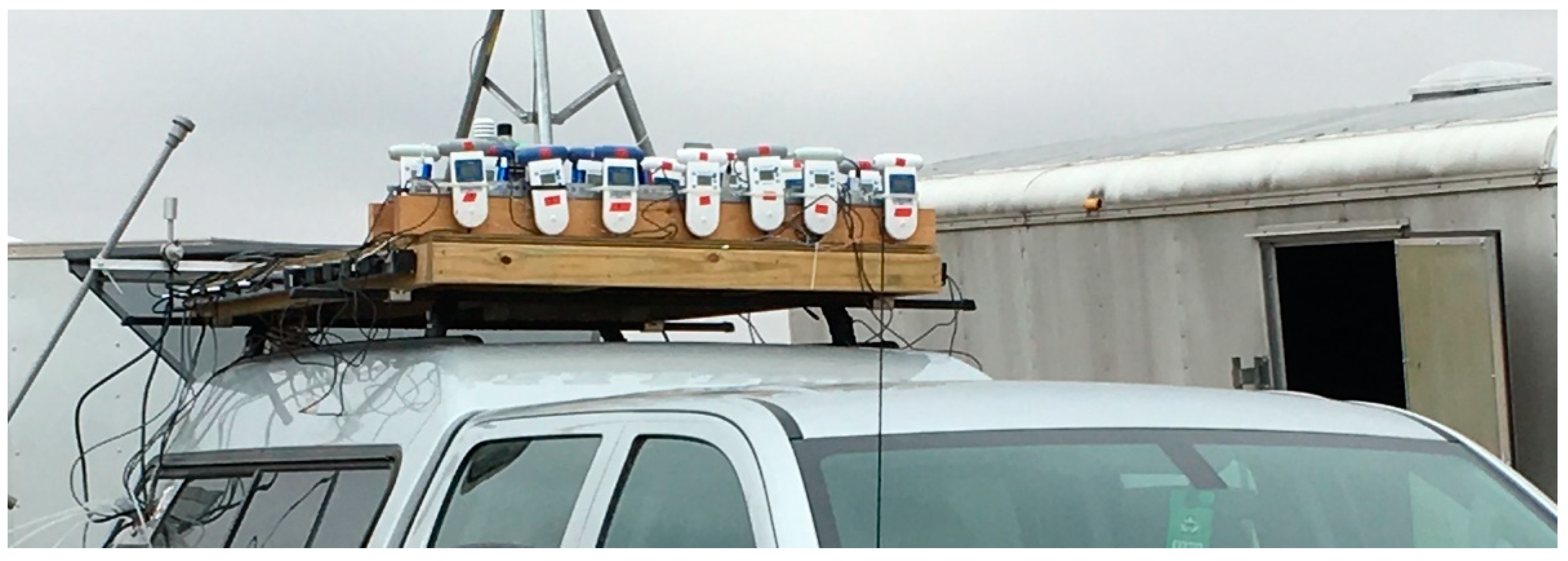
Cairpol and Aeroqual sensors were installed vertically onto the front of a custom vehicle rooftop sampling platform exposed directly to the smoke and near the reference instrument manifold (Figure 1, Figure 2 and Figure 3). For the March 2017 study, the sensor data were internally recorded on each sensor and downloaded nightly. For the November 2017 study, data from the Aeroqual sensors were output via 0–5 V analog output to a Dr DAS (Granville, OH, USA) Model Envidas Ultimate data acquisition system that simultaneously recorded measurements from the reference instrumentation. The Cairpol sensors were downloaded manually every evening.
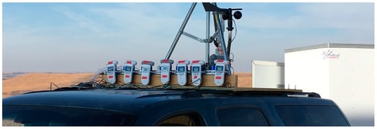
Figure 1.
Photograph of Aeroqual and Cairpol sensors attached to the roof of the sampling vehicle from the March 2017 Konza study.
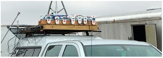
Figure 2.
Photograph of Aeroqual and Cairpol sensors attached to the roof of the sampling vehicle from the November 2017 Konza and Tallgrass studies.
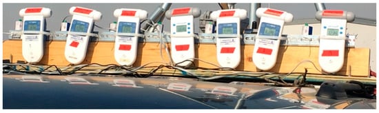
Figure 3.
Close-up photograph of Aeroqual and Cairpol sensors mounted to the roof of the sampling vehicle.
The Aeroqual sensors’ internal data download transmission was very slow for the early Model S500 handsets, making analog data acquisition preferable for longer field studies. The disadvantages of using analog output were potential precision loss in digital-to-analog or analog-to-digital conversions, especially for concentrations near the limits of detection. The 0–5 V output provided real-time data to our data acquisition system, whereas the on-handset data collection could only be viewed post hoc (although both the Cairpol and Aeroqual sensors displayed the most recent reading on the device itself). The on-handset data collection also recorded measurements higher than the maximum calibration range of the sensors, whereas the 0–5 V analog output maxed out (at 5 V) at the calibrated maximum. Another disadvantage of 0–5 V analog data collection in a mobile platform, particularly on rough terrain, was the possibility of connection issues developing (e.g., a bump jiggling loose a wire), although the on-handset data were always available as a backup if necessary.
The Aeroqual sensors were used as received (with the manufacturer’s calibration) for the March 2017 study but were recalibrated on 8 November 2017 before the November 2017 study. A post-study calibration check was also performed on 14 December 2017, shortly after the November study. The Cairpol sensors were factory-calibrated and could not be internally recalibrated by the user. The calibration of the Cairpol sensors was tested at the U.S. EPA laboratory on 18 December 2017, following the November 2017 study. The inability of the Cairpol sensors to allow end-user calibration is a potential issue, particularly for sensors whose performances degrade over time. The Cairpol sensors did have user-replaceable filters on the sensor inlet, which was particularly important in high particulate loading of smoke plumes. The Cairpol sensors also reported sensor temperature and relative humidity, which allows those parameters to be used in any potential corrections.
An overview of the sensors utilized during each study day is summarized in Table 3. We focused most of our discussion on the CO, CO2, and NO2 sensors for the following reasons. First, these sensors all measured specific species for which we had collocated reference instruments on the measurement platform. Although we had additional measurements of NH3 and H2S in the November studies, the NH3 measurements had a slow response (due to the “stickiness” of NH3 in the sampling system) and the H2S instrument had a large spectral interference from CO, which were not resolved before the study. The VOC and NMHC sensors measured groups of compounds (versus individual species), and the individual response for each species was different. In addition, we did not make comprehensive, speciated VOC or hydrocarbon measurements during the study beyond those we previously reported in [52].
Table 3.
Number and type of sensors used for each study period.
Although the O3 sensors worked well in nonplume conditions, they measured no O3 within the fire plumes. This was as expected due to titration by nitric oxide (NO) and is in agreement with our NO chemiluminescence FRM measurements of O3. Low O3 concentrations during these same burn campaigns were previously discussed in the context of UV photometric O3 instrument artifacts [53]. Making inferences on sensor performance under these smoke conditions with O3 concentrations in the range of 0–6 ppbv was not informative and, therefore, was not presented or discussed.
2.3. Missoula Fire Lab Controlled Burns
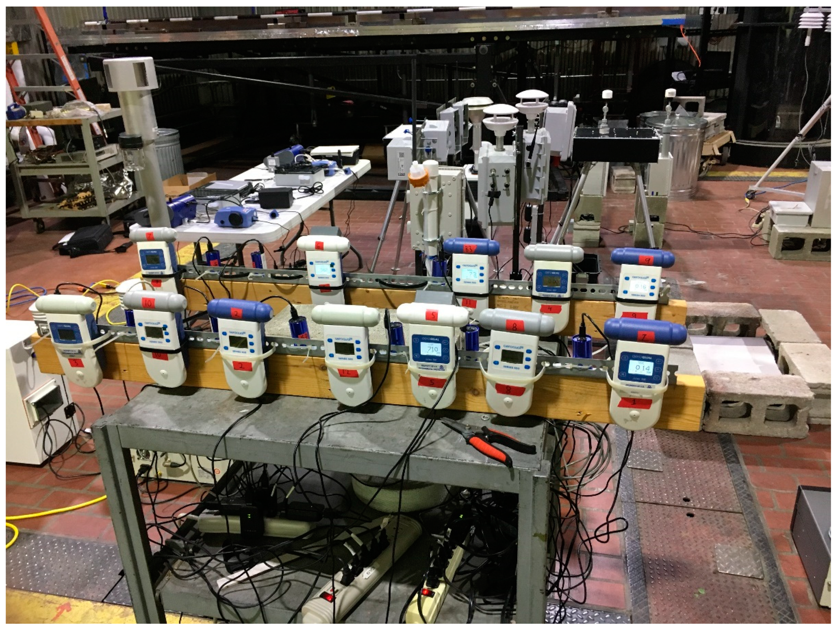
Controlled laboratory testing evaluated the sensors under simulated wildland fire exposure conditions at the USFS Rocky Mountain Research Station FSL combustion research facility in Missoula, Montana. Varying concentrations of smoke from fuel typical of the western U.S. under different combustion conditions (e.g., flaming and smoldering) were produced in the chamber, as described in [27]. A series of 33 burns was performed from 16–24 April 2018, and the fuel consisted of various combinations of Ponderosa pine needles and fine woody debris. The 12.4 m by 12.4 m by 19.6 m chamber (3000 m3) was ventilated with outdoor ambient air prior to each burn. The sensor testing was conducted using “static chamber” burns to simulate sensor exposure under in situ sampling conditions. The fuel was ignited in a closed chamber that was allowed to fill with smoke. Two large circulation fans mounted on the chamber walls and destratification fans on the chamber ceiling facilitated mixing and maintained homogenous smoke conditions during the tests. The reference instruments were in an adjacent observation room and sampled from the burn chamber through a Teflon™ PFA (Perfluoroalkoxy) tubing manifold extended through a port in the wall. The experimental details, fuels, and burn concentrations were described previously. We performed an integrated analysis of all 33 static chamber burns in this paper and did not evaluate burn-specific performance. A photograph of the Cairpol and Aeroqual sensor setup in the burn chamber is shown in Figure 4.
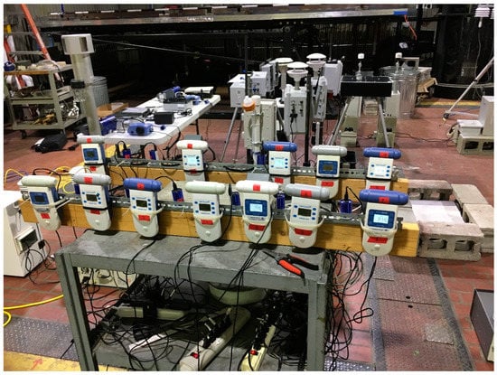
Figure 4.
Photograph of Aeroqual and Cairpol sensors in the FSL.
2.4. Statistical Evaluation of Sensor Performance
We used a variety of statistical metrics to assess the performances of the sensors under our testing conditions. For sensors for which we had collocated reference measurements (i.e., CO, CO2, and NO2), we compared the sensors to the reference measurements using both linear regression analysis and analysis of the sensor-versus-reference discrepancies. We removed all datapoints where the sensor measurements were above the maximum range of the sensors (i.e., 20 ppmv for the Cairpol CO sensors, 25 ppmv for the Aeroqual CO sensors, etc.). The ranges for each sensor are reported in Table 1. After removing this data, we performed an ordinary least squares linear regression of the sensor measurement (y) versus the reference measurement (x). We calculated the slope and intercept (and associated standard errors), as well as the coefficient of determination (r2).
The Cairpol sensors were used as-received with no additional calibration, whereas the Aeroqual sensors were used as-received in the March 2017 studies but were calibrated using reference gases prior to the November 2017 and Missoula (2018) studies. Only the CO, CO2, and NO2 sensors were calibrated—other species (e.g., VOC, NMHC, NH3, and H2S) were used as-received for all studies. We calculated sensor accuracy using the following equation [27]:
where X is the sensor measurement, and R is the associated reference measurement. We calculated ΔX = Xsensor − Xreference for each one-minute datapoint. From this, we calculated the median error (median ΔX) and mean bias error (MBE, mean ΔX) values for each study. We calculated the root mean square error (RMSE) as:
In cases where multiple CO or NO2 sensors of the same type (i.e., Cairpol or Aeroqual) were used on the same study day, we also looked at how well the duplicate sensors compared with each other. For this analysis, we calculated the collocated precision:
For duplicate sensors, we also calculated the coefficient of determination (r2) and the Deming regression statistics. We used the Deming regression in this case because of the similar uncertainties in the measurements from both sensors being compared. Because we were comparing duplicates of the same sensor, we assumed identical uncertainties (e.g., the ratio of the variances was 1), in which case the Deming regression was equivalent to an orthogonal regression. Ordinary least squares regression was justified in the sensor-versus-reference comparison given the assumed higher uncertainty in the sensor measurements versus the reference measurements.
3. Results and Discussion
3.1. Evaluation of Cairpol and Aeroqual CO Sensors
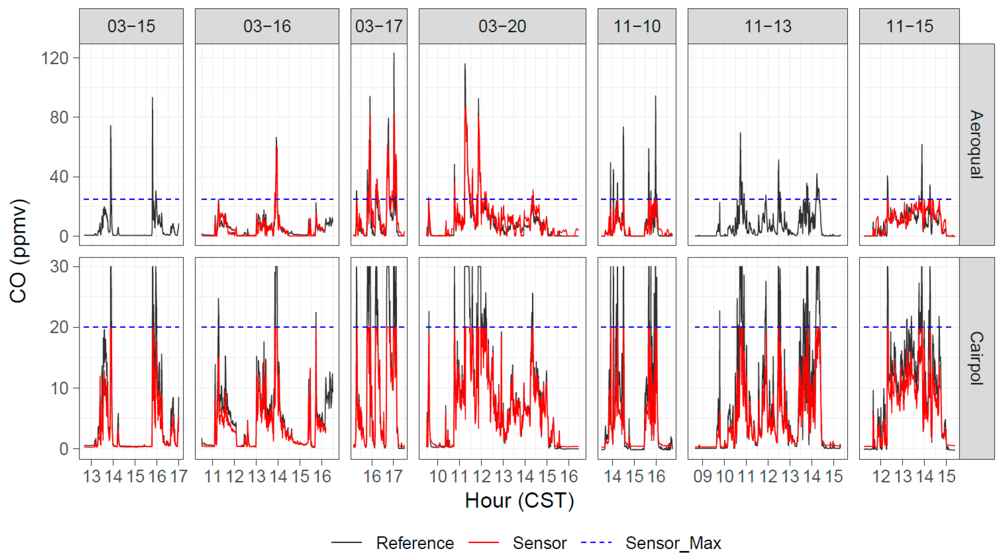
During the March and November prescribed fires at Konza Prairie and Tallgrass Prairie, the measured CO concentrations ranged from approximately 0 ppmv (during background periods) up to 123 ppmv. The Cairpol CO sensors had a limited range, from 0 ppmv to 20 ppmv, and did not report values higher than 20 ppmv. The Aeroqual CO sensors had a working range of 0 ppmv up to 25 ppmv, but they reported higher values than 25 ppmv if the Aeroqual sensor data were recorded on the handset and downloaded to a computer (as the data were collected for the March 2017 experiments). However, if the data were recorded on a data acquisition system (as for the November 2017 study) using a 0–5 V output, the maximum value that could be recorded was 25 ppmv. Although these ranges were limited for very near source measurements, such as some of the measurements made here (directly downwind of an active fireline), the measurement ranges were sufficient for assessing pollutant concentrations hundreds of meters to kilometers downwind of fires, such as in impacted communities [54]. In addition, even if the sensors do not give accurate measurements above their maximum values, they can still provide an indication of high CO levels, which could be useful for decision making by first responders.
A timeseries comparison of one of the Cairpol CO sensors (unit 2617) with reference CO measurements is shown in Figure 5. The large-scale (ppmv level) variability in the reference measurements was tracked well by the sensor measurements up to the sensor maximum reading of 20 ppmv.
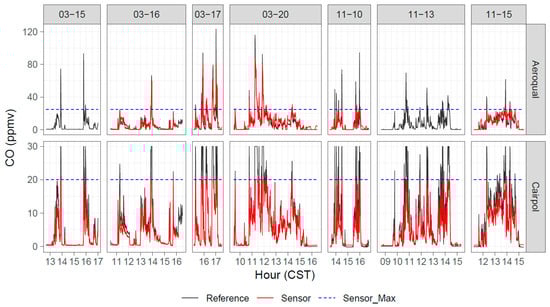
Figure 5.
Timeseries of reference, Aeroqual, and Cairpol CO measurements during seven days of Tallgrass Prairie prescribed burn experiments in 2017.
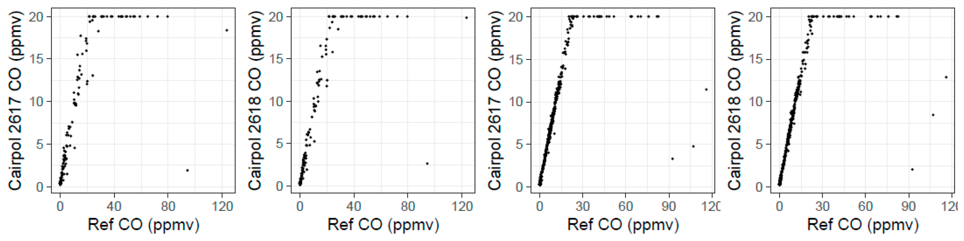
We removed all the data where the Cairpol sensor read 20 ppmv (the maximum value) under the assumption that this would remove all data where the Cairpol sensor was saturated. We then attempted ordinary least squares (OLS) linear regression for each Cairpol CO sensor versus the reference CO values. For the Spring 2017 study days, 15 March 2017 and 16 March 2017 provided strong correlations (r2 > 0.93); however, 17 March 2017 and 20 March 2017 showed poor correlations (r2 < 0.35). When we plotted each Cairpol CO sensor versus the reference CO measurements for those two days without removing any data (Figure 6), we observed that the Cairpol CO sensors did saturate at a reading of 20 ppmv. However, when CO levels reached higher than around 85 ppmv, the Cairpol sensors seemed to read lower values (i.e., below 20 ppmv). Of the fires we studied, one-minute CO concentrations only reached above 85 ppmv during these two study days, and it was always a transient response (i.e., lasted less than 2–3 min). The sensor drop could be due to the rapidly changing conditions when initially hit by a major plume or could be related to oversaturation of the sensors causing a false reading above a certain threshold value. Based on these results, we urge caution using Cairpol CO sensors at CO concentrations above 85 ppmv without additional study into what causes these false readings. We performed our statistical analysis of the Cairpol CO values versus Reference CO values both including these outlier points and after removing these two (for 3–17) or three (for 3–20) outlier points (Table A1 and Table A2).

Figure 6.
Timeseries of reference, Aeroqual, and Cairpol CO measurements during seven days of Tallgrass Prairie prescribed burn experiments in 2017.
After removing data with Cairpol CO above 20 ppmv (and the outlier points discussed above), the correlations between the Cairpol CO sensors and reference measurements were strong (Table A1 in Appendix A), with r2 ≥ 0.74 for all periods and r2 ≥ 0.90 for 9 of the 12 regressions. Only the 11–13 Tallgrass burns (and one of the two Cairpol CO sensors during the 11–10 Konza burns) had r2 < 0.90. There was variability in the regression slopes and intercepts from day to day, with a general trend of decreasing sensitivity (e.g., CO response versus CO exposure) over time among the March 2017, November 2017, and April 2018 studies. The reason for the sensitivity variations within each month was less clear, but may be related to ambient conditions (e.g., temperature and relative humidity) or plume-specific interferences. The 18 December 2017 laboratory calibration check of the two Cairpol CO sensors (zero air and CO reference gas span) produced readings of 4.1 ppmv and 4.4 ppmv for a reference concentration of 6.7 ppmv CO. This suggests that the laboratory CO response factor of the sensors was about 65%, which is similar to the response factors seen in the Tallgrass Prairie fires a month earlier (64—70%) but higher than the response seen during the 10 November 2017 Konza fire (48%). We assumed that the response factor was equal to the regression slope compared to the reference monitor. These responses were also smaller than the >86% responses seen during the 17 March 2017 and 20 March 2017 Konza studies. The degradation in sensor response over time was likely due to sensor aging.
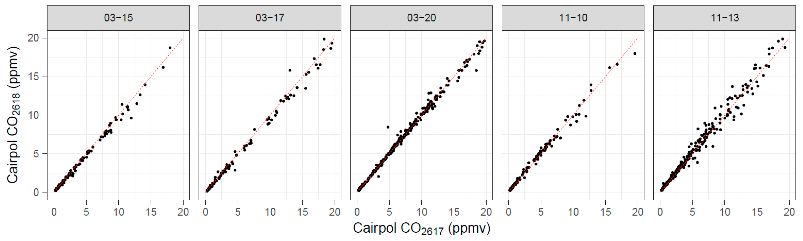
Duplicate Cairpol CO sensors gave excellent agreement and strong correlations (Figure 7), with collocated precisions better than 8% (Table 4). In addition, r2 > 0.99 for all the collocated Cairpol measurements, with Deming slopes within 5% of 1.0 and Deming intercepts within 10 ppbv (although the 95% confidence intervals for both slope and intercept did extend beyond these thresholds slightly).
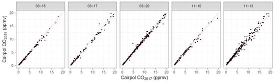
Figure 7.
Scatterplot comparing duplicate Cairpol CO sensors (Unit 2618 versus Unit 2617) for the five grassland burn days with valid data from both sensors.
Table 4.
Collocated precision, Deming regression statistics, and r2 values for duplicate sensors during the field studies.
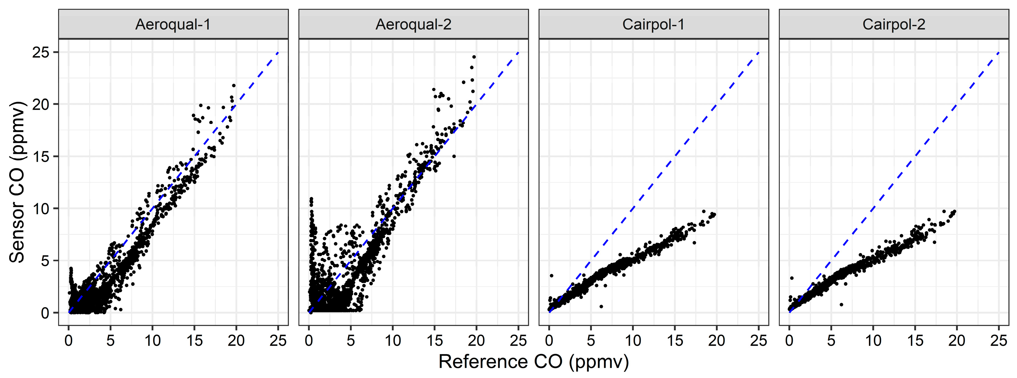
The merged Missoula chamber data (Figure 8, Table A1) gave excellent correlations (r2 ≥ 0.95 for Cairpol CO sensors). The FSL chamber data tested a range of burn conditions, including modified combustion efficiencies (MCEs) and concentration ranges [27]. Despite this, the overall coefficient of determination for the combined FSL chamber data was higher than most of the field burn days (Table A1). Some difference in performance between a laboratory versus field environment was expected. The CO sensors used in the Missoula study were just over one year old at the time of the study, so they had reached the end of their one-year manufacturer-recommended use period. Despite this, the readings were still strongly correlated with reference CO values. Consistent with the observation of decreased sensor response over time, the response of the sensors dropped to about 40% by the Missoula study. Thus, the Cairpol CO sensors seemed to perform relatively well within their calibration range, but they require regular calibration checks to address decreasing response over time due to sensor aging.
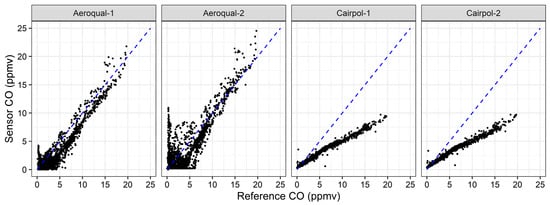
Figure 8.
Scatterplot of sensor CO measurements versus reference CO measurements for 33 experimental burns at the Fire Sciences Laboratory in 2018.
The Aeroqual CO measurement also tracked the reference measurement well (Figure 5), with reasonable correlations with the reference measurements (0.36 ≤ r2 ≤ 0.66). The highest correlations between the Aeroqual and reference CO measurements were for the Missoula chamber data (r2 = 0.74, 0.88; Figure 8). The sensitivity was higher than for the Cairpol instruments, although there were considerable intercept offsets for most of the regressions (up to 5.0 ppmv) with the manufacturer’s calibration. The ability to recalibrate the Aeroqual sensors (for both zero and span concentrations) by the user seemed critical to address calibration issues as-received from the manufacturer. The collocated precision for Aeroqual CO sensors (Table 4) was 12% to 29%, significantly higher than for the Cairpol CO sensors. However, the Deming slopes were within 1% of 1.0 for two of the three collocated sensor days, and the intercepts were within the ±0.1–0.2 ppmv range. Although the duplicate Aeroqual CO sensors seemed to roughly agree with each other, they were much noisier than the Cairpol CO sensors. A 14 December 2017 calibration check of the Aeroqual CO sensors showed readings of 27.8 ppmv and 31.1 ppmv for an actual CO concentration of 24.2 ppmv.
Overall, both the Cairpol and the Aeroqual CO sensors were excellent at measuring frequent and rapid CO concentration changes in the low ppmv concentration range, even in complex, dynamic, and mobile environments. These sensors could be used as general indicators of smoke impact during wildland fire events. Given the importance of CO (and changes in CO) in characterizing wildfire emissions and impact (e.g., calculating normalized excess emission ratios, or NEMRs), this makes CO sensors a valuable tool for wildland fire response, especially in downwind, impacted communities (where the 20 ppmv or 25 ppmv maximum values are not relevant). End-user calibration, ideally under typical measurement conditions, is necessary for the quantitative use of sensors, especially given the depressed response and response degradation over time for the Cairpol CO sensors and the generally poor as-received calibrations (including considerable offset values) of the Aeroqual CO sensors.
The 1st EuNetAir joint exercise in Aveiro, Portugal, found strong correlations (r2 of 0.53–0.87) between four different CO sensor nodes and reference CO measurements [55]. The study (which lasted from 13–27 October 2014) measured the mean and maximum reference CO concentrations (hour average) for 0.33 ppmv and 1.36 ppmv. The sensor packages in [55] generally contained CO sensors based on Alphasense B4 electrochemical CO sensors.
Jiao et al. [34] found that the adjusted r2 value for hourly sensor measurements versus reference CO measurements was significantly improved (0.63 to 0.75) when incorporating a sensor age term into their multiple linear regression model for an AQMesh CO sensor. This was a 110–111-day collocation of an AQMesh CO sensor with reference CO measurements at the South Dekalb regulatory monitoring site in suburban Atlanta, GA, USA, which had CO values reaching up to about 1.5 ppmv. It is difficult to make a direct comparison given the differences in sensor models and measurement conditions, but the change in CO sensor response over time appears to be similar (qualitatively) between our study and [34].
In contrast with our study and [34], a summary of a 2019 workshop held by the U.S. EPA discussing sensor targets for CO [25] mentioned that the factory calibrations of CO sensors were generally stable over the lifetime of the sensor. It is possible that constant exposure to extreme (smoke) conditions could be partially responsible for sensor degradation and decreased response over time.
3.2. Evaluation of Aeroqual CO2 Sensors
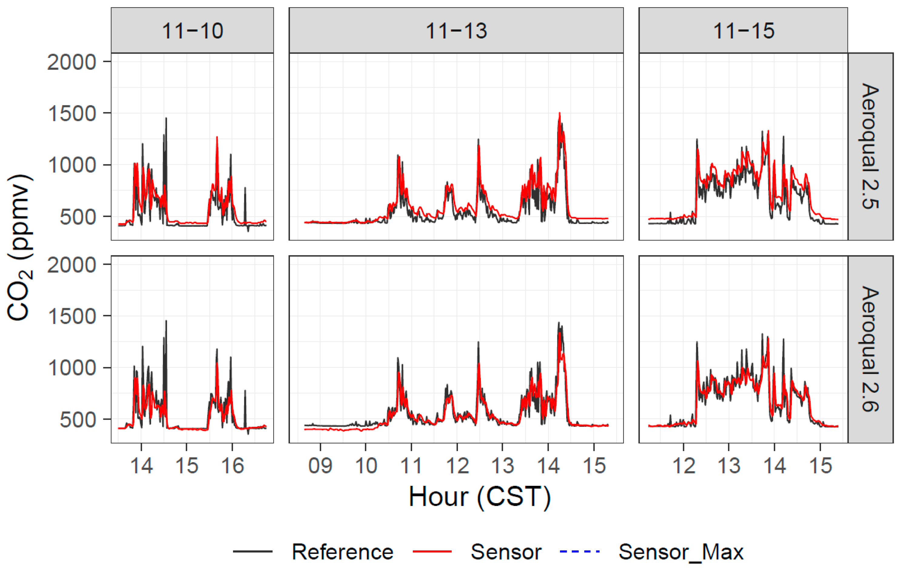
Aeroqual CO2 measurements were made during the November 2017 grassland burns and the 2018 Missoula chamber experiments. The Aeroqual CO2 measurements tracked reference CO2 measurements (Figure 9), with a possible positive offset. The r2 values for the Tallgrass burns and the Missoula burns were higher than 0.75, showing a strong correlation, although there was a positive offset (94–140 ppmv), as well as slopes less than unity (0.76–0.82), for the Tallgrass burns (Table A3). The sensors were recalibrated before the FSL chamber study, and the performance results were much better in terms of absolute agreement. Regressions for the combined FSL chamber data gave slopes of around 0.95 and intercepts between 1 and 2 ppmv for the duplicate CO2 sensors. The Konza burn (10 November 2017) produced r2 = 0.47 and 0.49, slopes of 0.49 and 0.60, and intercepts of 250 ppmv and 239 ppmv. Laboratory calibration checks of the Aeroqual CO2 sensors on 14 December 2017 showed readings of 2020 ppmv and 2120 ppmv for actual CO2 concentrations of 2000 ppmv.
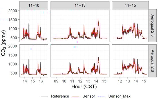
Figure 9.
Timeseries of reference and Aeroqual CO2 measurements during three days of Tallgrass Prairie prescribed burn experiments in 2017 when we had CO2 sensors present.
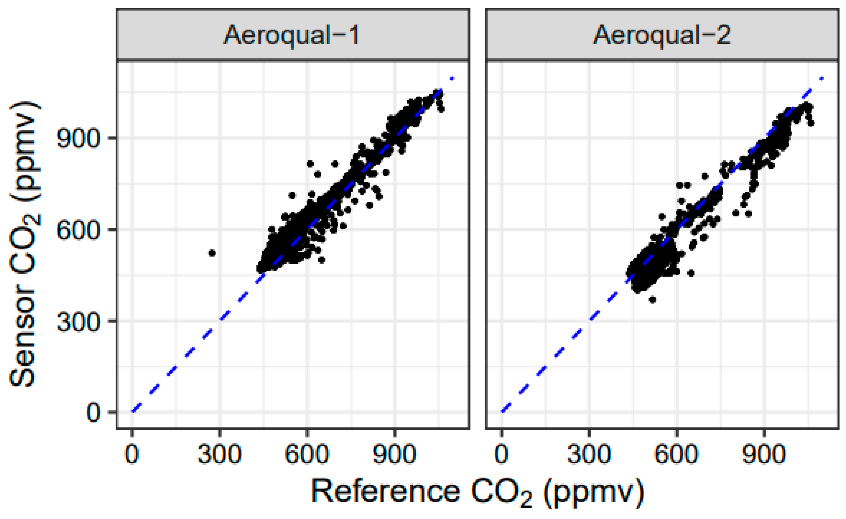
A scatterplot of sensor CO2 values versus reference CO2 values is shown in Figure 10 for the two Aeroqual CO2 units tested during the Missoula study. Like the Aeroqual CO sensors, the Aeroqual CO2 sensors showed a significant offset in the field when using as-received calibrations. In addition, the offset was different for the two different sensors. After calibration, however, the sensors tracked well with changes in environmental CO2, though the data were still noisy. For changes in the order of hundreds of ppmv larger, the Aeroqual CO2 sensors provided reasonable tracking of environmental CO2 concentrations; however, for CO2 changes in the order of tens of ppmv, the Aeroqual CO2 sensors struggled with resolving the signal from the sensor noise.
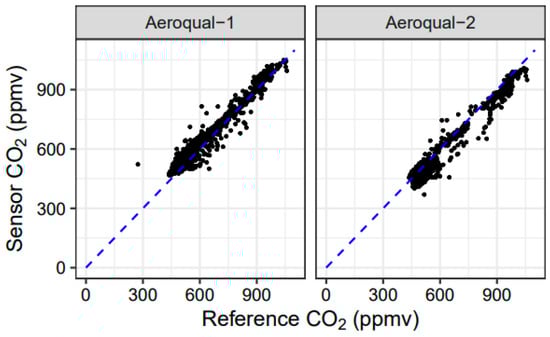
Figure 10.
Scatterplot of sensor CO2 measurements versus reference CO2 measurements for 33 experimental burns at the Fire Sciences Laboratory in 2018.
3.3. Evaluation of Cairpol and Aeroqual NO2 Sensors
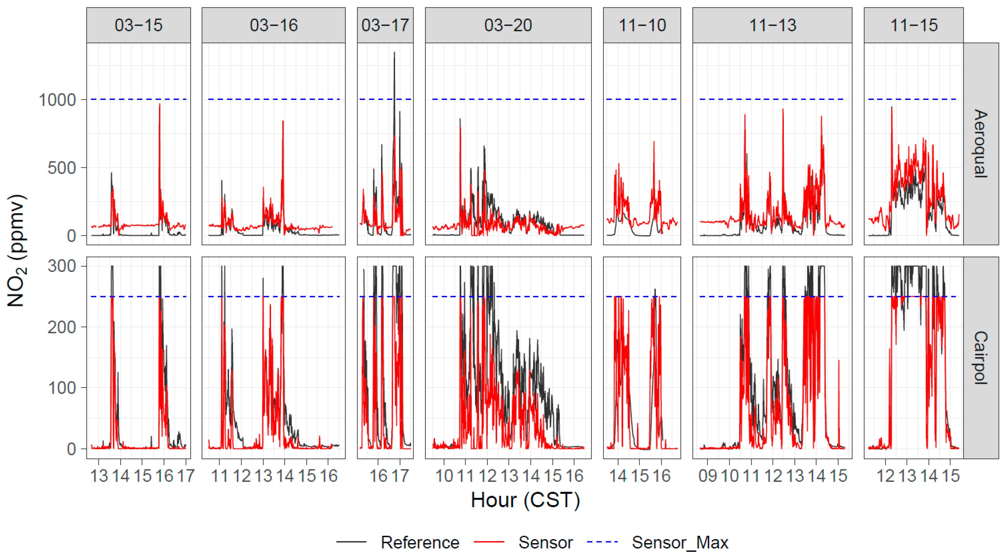
Cairpol NO2 sensors only measured up to 250 ppbv, which was less than the maximum values observed in the field studies (approximately 1 ppmv), but they showed reasonable correlations (0.70 ≤ r2 ≤ 0.93) to the measurable range in the field studies (Figure 11; Table A5). Despite strong correlations, the response factor was low, with linear regression slopes ranging from 0.35 to 0.88 and most below 0.70. The intercepts tended to be negative. It is important to note that there were no observed interferences from O3. Although O3 values are very low within the fire plume due to titration by NO [53], the readings were consistent with background NO2 during nonplume periods, even in the presence of up to 40 ppbv of O3. Cairpol NO2 sensors had r2 = 0.80 and 0.81 during the FSL chamber burn study, with slopes ranging from 0.65–0.66 and intercepts of −6.7 ppbv and −9.3 ppbv. A scatterplot of sensor NO2 versus reference NO2 for the Missoula burns is shown in Figure 12. The correlations between the Cairpol sensors and the CAPS NO2 instrument were poor at lower concentrations but improved at higher concentrations (>50 ppbv).
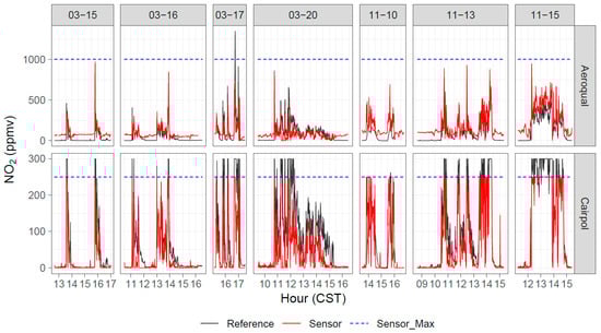
Figure 11.
Timeseries of reference, Aeroqual, and Cairpol NO2 measurements during seven days of Tallgrass Prairie prescribed burn experiments in 2017.
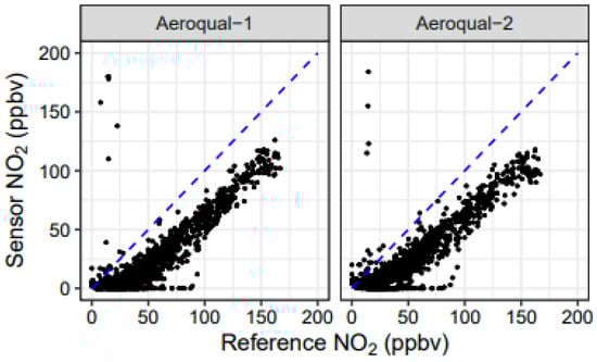
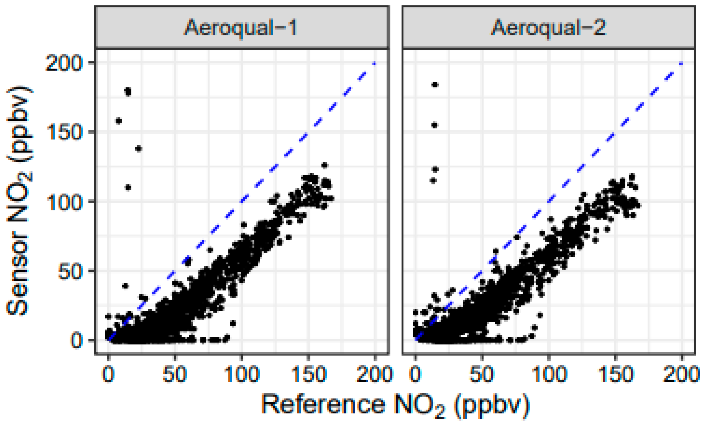
Figure 12.
Scatterplot of sensor NO2 measurements versus reference NO2 measurements for 33 experimental burns at the Fire Sciences Laboratory in 2018.
The Aeroqual NO2 sensors covaried well with the ambient NO2 (Figure 11 and Figure 12) but showed a positive artifact in the presence of O3 (even at low NO2 mixing ratios). This is a minor issue for fresh fire plume or laboratory experiments, as O3 is generally titrated to near zero immediately downwind of the emission source [53] but can be an issue further downwind. The r2 for the Fall 2017 burns was between 0.82 and 0.90, while the performance for the Spring burns was worse (r2 ≤ 0.62). It is likely that the O3 interference was more significant in March (with higher O3 levels) than in November, which caused the correlations to be better in the November study.
The collocated precision values for duplicate Cairpol and Aeroqual NO2 sensors are given in Table 5. The collocated precision for the Cairpol sensors was better than for the Aeroqual sensors, and the sensor-versus-sensor r2 > 0.97 for the Cairpol sensors. For the Aeroqual sensors, the correlations were generally worse (r2 < 0.93), the intercepts were much larger (suggesting a significant zero offset for the as-received duplicate sensors), and the collocated precision was worse (>28%). The collocated precision of the Cairpol NO2 sensors (12% to 19%) was higher than that of the Cairpol CO sensors (3% to 7%, Table 4), suggesting that NO2 in this low range (0–250 ppbv) was a noisier measurement for the sensors to make than CO in the 0–20 ppmv range. The significant discrepancies between precisions, slopes, intercepts, and r2 values for the Aeroqual versus Cairpol sensors suggest that the Cairpol sensors were more consistent in their as-received calibrations. The significant differences in the as-received calibrations between replicate Aeroqual sensors means that end-user calibration is especially important. Aeroqual does sell a calibration kit (add part number), and the S500 handsets allow sensor calibration using a zero and span linear model. This is essential for using the Aeroqual sensors tested here, given the internal inconsistencies between replicates. Cairpol, on the other hand, does not allow end-user calibration, but the as-received calibrations were generally consistent between replicate sensors.
Table 5.
Collocated precision, Deming regression statistics, and r2 values for duplicate NO2 sensors during the field studies.
Lin et al. [39] evaluated as-received Aeroqual series 500 O3 and NO2 monitors against reference analyzers for 2 months in Edinburgh, UK, and found good correlations (r2 = 0.91) between reference and sensor O3 measurements but poor correlations (r2 = 0.02) between reference and sensor NO2 measurements. However, they found that the Aeroqual NO2 data could be corrected by adding an offset term based on Aeroqual measured O3 data. This “corrected” Aeroqual NO2 provided much better correlations with the reference monitor (r2 = 0.88). Their as-received Aeroqual NO2 sensor head had a 20–30 ppbv offset compared to the reference monitor, even at zero O3 (Figures 3 and 4 in ref. [39]). Their analysis showed little correlation (r2 < 0.03) between the sensor versus reference discrepancy and relative humidity (RH) in the 30% to 100% range.
Masey et al. [56] also found strong agreement between reference and two Aeroqual NO2 measurements, but only when corrected for O3 concentrations. The authors discussed calibration and correction strategies for Aeroqual NO2 monitors to account for the O3 cross-sensitivities, including multiple training periods over time to encompass a degradation in sensor response over time. Response factor was a major issue with our March 2017 Konza NO2 measurements, with slopes (response factors) between 0.14 and 0.53. Some of the low response factors we observed in our regression analysis could be due to the influence of O3 interferences during nonfire periods, which would elevate the measured sensor NO2 at higher O3 (and lower reference NO2) values. This would shift the slope towards 0. The r2 values from these fires were also very poor (<0.53). Interestingly, the NO2 sensor we tested in the Fall 2017 Tallgrass fires performed much better, with r2 values of 0.85 and 0.90 and slopes of 0.90 and 1.02. This sensor head was newer, which may explain the higher slope (i.e., less response degradation from sensor aging).
In contrast to [39] and [56], Isiugo et al. [57] found that NO2 sensors performed poorly and could not fit the ±25% mean error NIOSH accuracy criterion. Even after training, they found that the Aeroqual NO2 sensor measurements had significant errors. Interestingly, the values measured in [57] were all below 40 ppbv, with meant NO2 concentrations of 4.6 ppbv and 9.4 ppbv for their training and testing datasets. These values, although typical of NO2 in the ambient air of many environments, are at the lower end of values measured in the other studies mentioned [39,56]. Similarly, Duvall et al. [33] found poor performance of Cairpol NO2 sensors versus reference instruments but also measured mostly lower concentrations.
In this study, we focused on fresh biomass burning plumes, where NO2 concentrations were elevated and O3 concentrations were near zero [53]. As a result, we did not have sufficient O3 cross-sensitivity data to generate an O3 correction. However, our experiment did present a potential scenario in which O3 corrections were less important. As the distance between the fresh emission plume and the sensor increases, the importance of an O3 correction increases. Even in biomass burning plumes, however, our results demonstrated that O3 corrections could be important for Aeroqual NO2 sensors [39,56]. In addition, we recommend using the same heads over their entire lifetime to better model the sensor degradation over time, as discussed in [56]. These are important factors for improving the accuracy of Aeroqual NO2 sensor measurements that were not fully accounted for the in the present study.
Both Cairpol and Aeroqual NO2 sensors listed chlorine (Cl2) as the major interference. Based on the low concentration of chlorinated VOCs measured during the grassland burn studies [52], we did not anticipate this interference to be significant in our setting. Although we noticed a significant O3 interference in the Aeroqual NO2 sensor used in this study (Model ENW), Aeroqual has since replaced their NO2 sensor with a newer sensor head model (Model END) for which the manufacturer claims improved O3 filtering performance [58].
3.4. Evaluation of Other Sensors
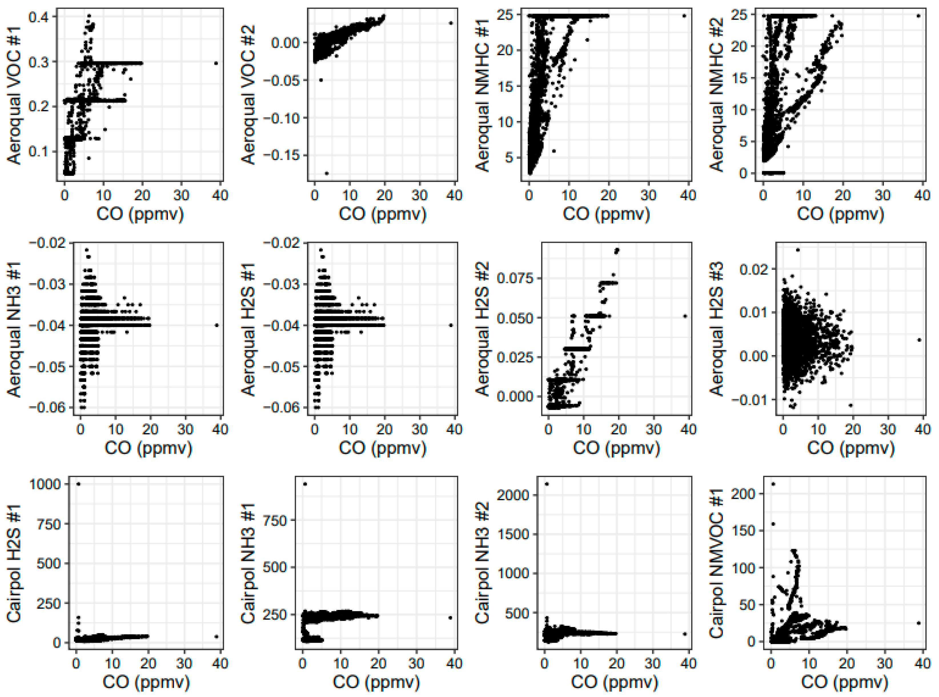
In addition to the Cairpol CO and NO2 sensors and the Aeroqual CO, CO2, and NO2 sensors, we also tested Aeroqual VOC (PID), NMHC (EC), H2S (EC), and NH3 (EC) sensor heads during the November 2017 study and the 2018 FSL study. In addition, we tested new Cairpol H2S, NH3, and NMVOC sensors. We did not have direct (1:1) reference equipment for these measurements during these studies, so we were unable to obtain an absolute comparison with reference measurements. In addition, the VOC, NMHC, and NMVOC sensors were nonspecific (i.e., they measure classes of compounds instead of individual compounds). However, we knew that these species (or compound classes) are emitted from biomass combustion. Therefore, as a first order “feasibility” check, we plotted the sensor data against reference CO data for the combined Missoula burns (Figure 13). Both the Aeroqual VOC sensors showed some correlation with CO, although one sensor showed better results than the other sensor. However, the sensor that showed better results also reported negative concentration values (which were determined based on voltages), suggesting that either the digital-to-analog converter (inside the sensor) or the analog-to-digital converter (as part of the data acquisition system) was operating near its lower limit or required additional calibration. It was not clear if the issue was noise within the sensor or the data acquisition system, so additional study is necessary to determine the behavior of the Aeroqual sensors’ analog outputs near their lower limits. Despite this, there appeared to be a reasonable correlation with a positive slope, as expected.
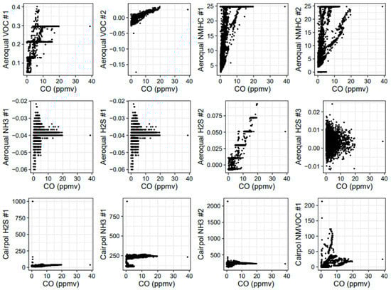
Figure 13.
Scatterplot of Aeroqual VOC, NMHC, H2S, and NH3 sensors and Cairpol H2S, NH3, and NMVOC sensors versus CO for the combined Fire Sciences Laboratory burns in 2018.
The Aeroqual NMHC sensors and the Cairpol NMVOC sensors, like the VOC sensors, also showed responses that increased as CO increased. However, unlike the VOC sensor behavior, the NMHC and NMVOC sensors’ relationships to CO varied from burn to burn. This suggests that there were variations in either NMHC or an interfering species that was measured by the NMHC sensors but not correlated with CO in the smoke. Both the NMHC sensors also maxed out above 25 ppmv during several burns. Because the NMHC sensors were nonspecific, it was uncertain exactly which species (in what ratio) the NMHC sensors were responding to. However, the high (25 ppmv) hydrocarbon concentrations were not measured by the Thermo Environmental Model 51i Total Hydrocarbon (THC) flame ionization detector (FID) instrument, which measured maximum values of 6.4 ppmv during the entire burn period. The NH3 and H2S sensors did not show a significant response during these tests, which represented very high near-fire smoke concentrations, indicating that these sensors would not provide useful information for this use case or in downwind communities.
4. Conclusions
In this study, we compared the responses of commercial, off-the-shelf CO, CO2, and NO2 sensors with reference equipment for fresh wildland fire plumes. The CO sensors performed the best but showed fire-specific response differences and a gradual decay in sensitivity over time. Of the CO sensors, the Cairpol sensors performed better as-received, whereas the Aeroqual sensors required additional calibration and resulted in noisier measurements. The Aeroqual CO2 sensors agreed with the reference CO2 measurements after calibration but had significant discrepancies out-of-the-box. The NO2 performance was better for the Cairpol sensors than the Aeroqual sensors but still lagged the CO and CO2 sensor performances in wildland-fire-relevant concentration ranges. The Aeroqual NO2 sensors had a positive O3 interference that did not appear to impact the more accurate Cairpol NO2 sensor measurements.
The performances of all the sensors were much better and more consistent during the FSL chamber “static burn” studies than when observed under real-world field conditions. It is likely that changing meteorological conditions (e.g., temperature and relative humidity), fuel- or combustion-specific variability in potential interfering compounds, and rapidly varying target pollutant concentrations contributed to the sensor measurement accuracy degradation observed during field testing.
The 2017 field studies were a precursor to the U.S. EPA’s Wildland Fire Sensor Challenge [27], whereas the 2018 chamber studies were carried out concurrently to the solver submission testing. The 2017 field studies provided a baseline for our understanding of commercial sensor performance in wildland fire plumes, particularly with respect to CO and CO2. Since the present study and [27], we have continued the evaluation of portable, small-form instruments and sensor packages for wildland fire plumes (both in chamber and field environments) and at smoke-impacted community monitoring sites for use as rapid deployment tools during wildland fire events.
Author Contributions
Conceptualization, R.W.L., S.P.U. and M.S.L.; methodology, A.R.W., R.W.L., S.P.U. and M.S.L.; software, A.R.W., R.W.L. and M.S.L.; validation, A.R.W., R.W.L., A.H. and M.S.L.; formal analysis, A.R.W. and M.S.L.; investigation, A.R.W., R.W.L., S.P.U., M.C., A.H. and M.S.L.; resources, R.L, S.P.U. and M.S.L.; data curation, M.S.L.; writing—original draft preparation, A.R.W.; writing—review and editing, A.R.W., R.W.L., S.P.U., M.C. and M.S.L.; visualization, A.R.W.; supervision, R.W.L., S.P.U. and M.S.L.; project administration, R.W.L., S.P.U. and M.S.L.; funding acquisition, R.W.L., S.P.U. and M.S.L. All authors have read and agreed to the published version of the manuscript.
Funding
This research received no external funding.
Institutional Review Board Statement
Not applicable.
Informed Consent Statement
Not applicable.
Data Availability Statement
Raw data will be available on data.gov and at https://doi.org/10.23719/1526477 (accessed on 30 March 2022) following the final publication of the manuscript.
Acknowledgments
We thank Brian Gullett from the Office of Research and Development at the United States Environmental Protection Agency (U.S. EPA) for his assistance with logistics and planning. We appreciate the support of U.S. EPA Region 7 on the ground in Kansas. We especially thank the staff and volunteers at the Konza Prairie Biological Station, whose gracious assistance in hosting us, as well as planning and executing the burns, made this study a success. We would also like to thank Cortina Johnson, Shaibal Mukerjee, and Libby Nessley from U.S. EPA for their internal reviews of the manuscript, as well as the anonymous reviewers.
Conflicts of Interest
The authors declare no conflict of interest. The views expressed in this article are those of the authors and do not necessarily represent the views or policies of the U.S. Environmental Protection Agency. Any mention of trade names, products, or services does not imply an endorsement by the U.S. Government or the U.S. Environmental Protection Agency. The EPA does not endorse any commercial products, services, or enterprises.
Appendix A
Table A1.
Regression statistics for CO sensors versus reference instruments.
Table A1.
Regression statistics for CO sensors versus reference instruments.
| Period | Sensor | r2 | Slope | se | Intercept | se | N |
|---|---|---|---|---|---|---|---|
| Konza (15 March 2017) | Cairpol CO (2617) | 0.94 | 0.591 | 0.009 | 0.075 | 0.059 | 256 |
| Konza (15 March 2017) | Cairpol CO (2618) | 0.96 | 0.574 | 0.008 | 0.057 | 0.048 | 256 |
| Konza (16 March 2017) | Cairpol CO (2617) | 0.94 | 0.715 | 0.010 | 0.177 | 0.060 | 335 |
| Konza (17 March 2017) | Cairpol CO (2617) | 0.30 | 0.202 | 0.029 | 3.605 | 0.490 | 116 |
| Konza (17 March 2017) | Cairpol CO (2618) | 0.34 | 0.211 | 0.028 | 3.359 | 0.469 | 116 |
| 1 Konza (17 March 2017) | Cairpol CO (2617) | 0.93 | 0.782 | 0.021 | 0.607 | 0.183 | 114 |
| 1 Konza (17 March 2017) | Cairpol CO (2618) | 0.95 | 0.775 | 0.016 | 0.445 | 0.143 | 114 |
| Konza (20 March 2017) | Cairpol CO (2617) | 0.32 | 0.270 | 0.020 | 3.549 | 0.244 | 390 |
| Konza (20 March 2017) | Cairpol CO (2618) | 0.34 | 0.278 | 0.020 | 3.519 | 0.240 | 390 |
| 1 Konza (20 March 2017) | Cairpol CO (2617) | 0.99 | 0.782 | 0.004 | 0.360 | 0.029 | 187 |
| 1 Konza (20 March 2017) | Cairpol CO (2618) | 0.99 | 0.775 | 0.004 | 0.394 | 0.030 | 188 |
| Konza (10 November 2017) | Cairpol CO (2617) | 0.87 | 0.442 | 0.013 | 0.844 | 0.114 | 187 |
| Konza (10 November 2017) | Cairpol CO (2618) | 0.92 | 0.490 | 0.011 | 0.748 | 0.094 | 188 |
| Tallgrass (13 November 2017) | Cairpol CO (2617) | 0.81 | 0.531 | 0.013 | 0.907 | 0.121 | 387 |
| Tallgrass (13 November 2017) | Cairpol CO (2618) | 0.75 | 0.512 | 0.015 | 1.105 | 0.140 | 386 |
| Tallgrass (15 November 2017) | Cairpol CO (2617) | 0.95 | 0.674 | 0.010 | 0.652 | 0.109 | 246 |
| Konza (16 March 2017) | Aeroqual CO (1.8) | 0.66 | 0.803 | 0.032 | −0.127 | 0.193 | 336 |
| Konza (16 March 2017) | Aeroqual CO (1.9) | 0.45 | 0.621 | 0.037 | 0.196 | 0.239 | 357 |
| Konza (17 March 2017) | Aeroqual CO (1.8) | 0.36 | 0.429 | 0.055 | 5.037 | 0.700 | 110 |
| Konza (17 March 2017) | Aeroqual CO (1.9) | 0.43 | 0.452 | 0.049 | 4.381 | 0.646 | 116 |
| Konza (20 March 2017) | Aeroqual CO (1.8) | 0.50 | 0.686 | 0.035 | 2.913 | 0.318 | 383 |
| Konza (20 March 2017) | Aeroqual CO (1.9) | 0.41 | 0.643 | 0.039 | 3.482 | 0.355 | 384 |
| Konza (10 November 2017) | Aeroqual CO (2.10) | 0.53 | 0.401 | 0.027 | 2.613 | 0.389 | 196 |
| 2 Tallgrass (13 November 2017) | Aeroqual CO (2.8) | 0.43 | 0.00066 | 0.000038 | 0.028 | 0.0005 | 401 |
| 2 Tallgrass (15 November 2017) | Aeroqual CO (2.8) | 0.60 | 0.00151 | 0.000078 | 0.015 | 0.001 | 251 |
| Tallgrass (15 November 2017) | Aeroqual CO (2.10) | 0.59 | 0.692 | 0.036 | 3.869 | 0.461 | 251 |
| Missoula (2018) | Cairpol CO (2617) | 0.96 | 0.470 | 0.0016 | 0.407 | 0.0075 | 3185 |
| Missoula (2018) | Cairpol CO (2618) | 0.96 | 0.467 | 0.016 | 0.449 | 0.0074 | 3185 |
| Missoula (2018) | Aeroqual (3.8) | 0.88 | 0.897 | 0.0060 | −0.933 | 0.028 | 3185 |
| Missoula (2018) | Aeroqual (3.10) | 0.74 | 0.924 | 0.0098 | −0.668 | 0.046 | 3185 |
1 Calculations after removing outlier points (see discussion in main text, Section 3.1). 2 There seemed to be a scaling issue with this data based on the data acquisition system setup because the sensor and reference data were correlated but at a factor of ~500 too small.
Table A2.
Sensor versus reference difference statistics for CO.
Table A2.
Sensor versus reference difference statistics for CO.
| Period | Sensor | Accuracy | Median ΔX | Mean ΔX | RMSE |
|---|---|---|---|---|---|
| Konza (15 March 2017) | Cairpol CO (2617) | 61.30% | −0.236 | −1.289 | 2.675 |
| Konza (15 March 2017) | Cairpol CO (2618) | 59.10% | −0.239 | −1.362 | 2.748 |
| Konza (16 March 2017) | Cairpol CO (2617) | 75.94% | −0.454 | −0.971 | 1.722 |
| Konza (17 March 2017) | Cairpol CO (2617) | 68.83% | 0.074 | −2.313 | 13.157 |
| Konza (17 March 2017) | Cairpol CO (2618) | 66.42% | −0.026 | −2.492 | 12.996 |
| 1 Konza (17 March 2017) | Cairpol CO (2617) | 88.96% | 0.083 | −0.623 | 2.187 |
| 1 Konza (17 March 2017) | Cairpol CO (2618) | 85.39% | −0.018 | −0.824 | 2.087 |
| Konza (20 March 2017) | Cairpol CO (2617) | 82.17% | −0.168 | −1.146 | 8.734 |
| Konza (20 March 2017) | Cairpol CO (2618) | 82.54% | −0.125 | −1.122 | 8.618 |
| 1 Konza (20 March 2017) | Cairpol CO (2617) | 93.12% | −0.165 | −0.39 | 0.942 |
| 1 Konza (20 March 2017) | Cairpol CO (2618) | 93.38% | −0.123 | −0.374 | 0.957 |
| Konza (10 November 2017) | Cairpol CO (2617) | 62.81% | 0.296 | −1.686 | 4.856 |
| Konza (10 November 2017) | Cairpol CO (2618) | 65.30% | 0.302 | −1.591 | 4.327 |
| Tallgrass (13 November 2017) | Cairpol CO (2617) | 69.54% | −0.071 | −1.679 | 4.326 |
| Tallgrass (13 November 2017) | Cairpol CO (2618) | 71.33% | 0.115 | −1.573 | 4.542 |
| Tallgrass (15 November 2017) | Cairpol CO (2617) | 75.22% | −1.745 | −2.057 | 3.349 |
| Konza (16 March 2017) | Aeroqual CO (1.8) | 77.29% | −0.670 | −0.943 | 2.911 |
| Konza (16 March 2017) | Aeroqual CO (1.9) | 66.41% | −0.730 | −1.512 | 4.022 |
| Konza (17 March 2017) | Aeroqual CO (1.8) | 82.49% | 1.960 | 1.183 | 8.785 |
| Konza (17 March 2017) | Aeroqual CO (1.9) | 95.45% | 1.020 | 0.336 | 8.338 |
| Konza (20 March 2017) | Aeroqual CO (1.8) | 81.86% | 0.360 | 1.067 | 5.314 |
| Konza (20 March 2017) | Aeroqual CO (1.9) | 76.40% | 0.600 | 1.387 | 5.977 |
| Konza (10 November 2017) | Aeroqual CO (2.10) | 80.53% | 0.189 | −1.260 | 9.210 |
| 2 Tallgrass (13 November 2017) | Aeroqual CO (2.8) | 0.48% | −2.665 | −6.604 | 11.730 |
| 2 Tallgrass (15 November 2017) | Aeroqual CO (2.8) | 0.32% | −8.567 | −8.908 | 12.442 |
| Tallgrass (15 November 2017) | Aeroqual CO (2.10) | 87.48% | 0.245 | 1.119 | 5.754 |
| Missoula (2018) | Cairpol CO (2617) | 59.93% | −0.700 | −1.265 | 2.236 |
| Missoula (2018) | Cairpol CO (2618) | 60.88% | −0.664 | −1.235 | 2.229 |
| Missoula (2018) | Aeroqual (3.8) | 60.11% | −1.364 | −1.259 | 1.746 |
| Missoula (2018) | Aeroqual (3.10) | 71.21% | −1.086 | −0.909 | 2.118 |
1 Calculations after removing outlier points (see discussion in main text, Section 3.1). 2 There seemed to be a scaling issue with this data based on the data acquisition system setup because the sensor and reference data were correlated but at a factor of ~500 too small.
Table A3.
Regression statistics for CO2 sensors versus reference instruments.
Table A3.
Regression statistics for CO2 sensors versus reference instruments.
| Period | Sensor | r2 | Slope | se | Intercept | se | N |
|---|---|---|---|---|---|---|---|
| Konza (10 November 2017) | Aeroqual CO2 (2.5) | 0.49 | 0.602 | 0.045 | 238.829 | 24.984 | 196 |
| Konza (10 November 2017) | Aeroqual CO2 (2.6) | 0.47 | 0.488 | 0.037 | 250.211 | 20.957 | 196 |
| Tallgrass (13 November 2017) | Aeroqual CO2 (2.5) | 0.77 | 0.906 | 0.025 | 94.036 | 14.086 | 401 |
| Tallgrass (13 November 2017) | Aeroqual CO2 (2.6) | 0.76 | 0.788 | 0.022 | 101.793 | 12.524 | 401 |
| Tallgrass (15 November 2017) | Aeroqual CO2 (2.5) | 0.82 | 0.900 | 0.027 | 130.208 | 18.994 | 251 |
| Tallgrass (15 November 2017) | Aeroqual CO2 (2.6) | 0.81 | 0.804 | 0.024 | 128.756 | 17.090 | 251 |
| Missoula (2018) | Aeroqual CO2 (3.5) | 0.97 | 0.948 | 0.0029 | 1.672 | 1.672 | 3185 |
| 1 Missoula (2018) | Aeroqual CO2 (3.6) | 0.94 | 0.948 | 0.0056 | 1.804 | 3.258 | 1779 |
1 Aeroqual CO2 (3.6) was not operating during all of the burns. Only data for which the sensor was operating are included in this analysis.
Table A4.
Sensor versus reference difference statistics for CO2.
Table A4.
Sensor versus reference difference statistics for CO2.
| Period | Sensor | Accuracy | Median ΔX | Mean ΔX | RMSE |
|---|---|---|---|---|---|
| Konza (10 November 2017) | Aeroqual CO2 (2.5) | 94.47% | 28.233 | 29.148 | 144.225 |
| Konza (10 November 2017) | Aeroqual CO2 (2.6) | 96.22% | −1.633 | −19.946 | 141.399 |
| Tallgrass (13 November 2017) | Aeroqual CO2 (2.5) | 92.12% | 40.600 | 42.841 | 97.389 |
| Tallgrass (13 November 2017) | Aeroqual CO2 (2.6) | 97.57% | −10.833 | −13.181 | 85.827 |
| Tallgrass (15 November 2017) | Aeroqual CO2 (2.5) | 90.40% | 54.267 | 63.677 | 117.199 |
| Tallgrass (15 November 2017) | Aeroqual CO2 (2.6) | 99.81% | 8.767 | −1.249 | 96.718 |
| Missoula (2018) | Aeroqual CO2 (3.5) | 95.46% | 29.300 | 25.544 | 32.246 |
| 1 Missoula (2018) | Aeroqual CO2 (3.6) | 95.11% | −31.700 | −27.579 | 41.277 |
1 Aeroqual CO2 (3.6) was not operating during all of the burns. Only data for which the sensor was operating are included in this analysis.
Table A5.
Regression statistics for NO2 sensors versus reference instruments.
Table A5.
Regression statistics for NO2 sensors versus reference instruments.
| Period | Sensor | r2 | Slope | se | Intercept | se | N |
|---|---|---|---|---|---|---|---|
| Konza (15 March 2017) | Cairpol NO2 (2057) | 0.93 | 0.615 | 0.011 | −2.307 | 0.665 | 256 |
| Konza (15 March 2017) | Cairpol NO2 (2058) | 0.93 | 0.566 | 0.010 | −2.870 | 0.638 | 256 |
| Konza (16 March 2017) | Cairpol NO2 (2057) | 0.73 | 0.707 | 0.024 | −5.464 | 1.462 | 335 |
| Konza (16 March 2017) | Cairpol NO2 (2058) | 0.74 | 0.685 | 0.022 | −6.625 | 1.358 | 335 |
| Konza (17 March 2017) | Cairpol NO2 (2057) | 0.76 | 0.376 | 0.020 | 0.249 | 3.139 | 119 |
| Konza (17 March 2017) | Cairpol NO2 (2058) | 0.72 | 0.391 | 0.022 | −0.413 | 3.550 | 119 |
| Konza (20 March 2017) | Cairpol NO2 (2057) | 0.70 | 0.368 | 0.012 | −2.270 | 1.594 | 416 |
| Konza (20 March 2017) | Cairpol NO2 (2058) | 0.70 | 0.358 | 0.012 | −4.601 | 1.443 | 413 |
| Konza (10 November 2017) | Cairpol NO2 (2061) | 0.90 | 0.565 | 0.014 | 0.293 | 2.032 | 186 |
| Tallgrass (13 November 2017) | Cairpol NO2 (2062) | 0.84 | 0.685 | 0.016 | −5.295 | 1.573 | 360 |
| Tallgrass (15 November 2017) | Cairpol NO2 (2062) | 0.90 | 0.884 | 0.025 | −1.341 | 2.743 | 149 |
| Konza (15 March 2017) | Aeroqual NO2 (1.1) | 0.42 | 0.458 | 0.034 | 164.83 | 3.127 | 261 |
| Konza (15 March 2017) | Aeroqual NO2 (1.7) | 0.37 | 0.504 | 0.042 | 73.309 | 3.912 | 257 |
| Konza (16 March 2017) | Aeroqual NO2 (1.1) | 0.51 | 0.66 | 0.035 | 135.471 | 3.006 | 340 |
| Konza (16 March 2017) | Aeroqual NO2 (1.7) | 0.64 | 0.764 | 0.031 | 51.985 | 2.613 | 343 |
| Konza (17 March 2017) | Aeroqual NO2 (1.1) | 0.45 | 0.313 | 0.030 | 144.433 | 8.129 | 131 |
| Konza (17 March 2017) | Aeroqual NO2 (1.7) | 0.56 | 0.406 | 0.032 | 52.863 | 8.463 | 131 |
| Konza (20 March 2017) | Aeroqual NO2 (1.1) | 0.09 | 0.138 | 0.022 | 137.42 | 3.116 | 419 |
| Konza (20 March 2017) | Aeroqual NO2 (1.7) | 0.20 | 0.243 | 0.024 | 47.322 | 3.409 | 419 |
| Konza (10 November 2017) | Aeroqual NO2 (2.4) | 0.88 | 0.602 | 0.016 | 91.963 | 3.076 | 196 |
| Tallgrass (13 November 2017) | Aeroqual NO2 (2.4) | 0.82 | 0.878 | 0.020 | 72.332 | 3.485 | 401 |
| Tallgrass (15 November 2017) | Aeroqual NO2 (2.4) | 0.90 | 1.023 | 0.022 | 103.919 | 5.575 | 251 |
| Missoula (2018) | Cairpol NO2 (2059) | 0.80 | 0.659 | 0.0058 | −9.317 | 0.275 | 3180 |
| Missoula (2018) | Cairpol NO2 (2061) | 0.81 | 0.649 | 0.0055 | −6.730 | 0.259 | 3183 |
Table A6.
Sensor versus reference difference statistics for NO2.
Table A6.
Sensor versus reference difference statistics for NO2.
| Period | Sensor | Accuracy | Median ΔX | Mean ΔX | RMSE |
|---|---|---|---|---|---|
| Konza (15 March 2017) | Cairpol NO2 (2057) | 51.67% | −1.100 | −11.361 | 26.130 |
| Konza (15 March 2017) | Cairpol NO2 (2058) | 44.59% | −1.700 | −13.277 | 30.141 |
| Konza (16 March 2017) | Cairpol NO2 (2057) | 54.68% | −4.000 | −15.409 | 30.825 |
| Konza (16 March 2017) | Cairpol NO2 (2058) | 49.03% | −4.200 | −17.331 | 31.325 |
| Konza (17 March 2017) | Cairpol NO2 (2057) | 37.83% | −18.400 | −58.403 | 102.800 |
| Konza (17 March 2017) | Cairpol NO2 (2058) | 38.63% | −19.800 | −57.647 | 101.897 |
| Konza (20 March 2017) | Cairpol NO2 (2057) | 34.18% | −47.800 | −57.213 | 89.061 |
| Konza (20 March 2017) | Cairpol NO2 (2058) | 30.31% | −54.300 | −58.272 | 86.265 |
| Konza (10 November 2017) | Cairpol NO2 (2061) | 56.88% | −5.416 | −35.080 | 68.118 |
| Tallgrass (13 November 2017) | Cairpol NO2 (2062) | 59.65% | −11.555 | −24.255 | 41.646 |
| Tallgrass (15 November 2017) | Cairpol NO2 (2062) | 86.33% | −1.060 | −8.855 | 30.377 |
| Konza (15 March 2017) | Aeroqual NO2 (1.1) | −354.40% | 160.600 | 147.256 | 161.744 |
| Konza (15 March 2017) | Aeroqual NO2 (1.7) | −73.24% | 69.600 | 56.995 | 92.618 |
| Konza (16 March 2017) | Aeroqual NO2 (1.1) | −197.88% | 125.900 | 121.605 | 133.320 |
| Konza (16 March 2017) | Aeroqual NO2 (1.7) | −4.66% | 47.700 | 42.407 | 62.438 |
| Konza (17 March 2017) | Aeroqual NO2 (1.1) | 70.94% | 114.300 | 42.951 | 177.002 |
| Konza (17 March 2017) | Aeroqual NO2 (1.7) | 76.31% | 19.800 | −35.011 | 159.105 |
| Konza (20 March 2017) | Aeroqual NO2 (1.1) | 35.07% | 79.500 | 59.023 | 123.402 |
| Konza (20 March 2017) | Aeroqual NO2 (1.7) | 76.31% | −6.500 | −21.533 | 102.768 |
| Konza (10 November 2017) | Aeroqual NO2 (2.4) | 51.33% | 80.284 | 50.581 | 89.443 |
| Tallgrass (13 November 2017) | Aeroqual NO2 (2.4) | 37.20% | 68.963 | 60.587 | 85.136 |
| Tallgrass (15 November 2017) | Aeroqual NO2 (2.4) | 40.70% | 111.203 | 108.070 | 123.970 |
| Missoula (2018) | Cairpol NO2 (2059) | 39.85% | −19.300 | −21.507 | 25.939 |
| Missoula (2018) | Cairpol NO2 (2061) | 46.06% | −16.800 | −19.275 | 24.030 |
References
- Baron, R.; Saffell, J. Amperometric Gas Sensors as a Low Cost Emerging Technology Platform for Air Quality Monitoring Applications: A Review. ACS Sens. 2017, 2, 1553–1566. [Google Scholar] [CrossRef] [PubMed]
- Karagulian, F.; Barbiere, M.; Kotsev, A.; Spinelle, L.; Gerboles, M.; Lagler, F.; Redon, N.; Crunaire, S.; Borowiak, A. Review of the Performance of Low-Cost Sensors for Air Quality Monitoring. Atmosphere 2019, 10, 506. [Google Scholar] [CrossRef] [Green Version]
- Malings, C.; Tanzer, R.; Hauryliuk, A.; Kumar, S.P.N.; Zimmerman, N.; Kara, L.B.; Presto, A.A.; Subramanian, R. Development of a general calibration model and long-term performance evaluation of low-cost sensors for air pollutant gas monitoring. Atmos. Meas. Tech. 2019, 12, 903–920. [Google Scholar] [CrossRef] [Green Version]
- Williams, R.; Kaufman, A.; Hanley, T.; Rice, J.; Garvey, S. Evaluation of field-Deployed Low Cost PM Sensors; U.S. Environmental Protection Agency: Washington, DC, USA, 2014; EPA/600/R-14/464 (NTIS PB 2015-102104).
- Williams, R.; Kilaru, V.; Snyder, E.; Kaufman, A.; Dye, T.; Rutter, A.; Russell, A.; Hafner, H. Air Sensor Guidebook; U.S. Environmental Protection Agency: Washington, DC, USA, 2014; EPA/600/R-14/159 (NTIS PB2015-100610).
- Snyder, E.G.; Watkins, T.H.; Solomon, P.A.; Thoma, E.D.; Williams, R.W.; Hagler, G.S.W.; Shelow, D.; Hindin, D.A.; Kilaru, V.J.; Preuss, P.W. The Changing Paradigm of Air Pollution Monitoring. Environ. Sci. Technol. 2013, 47, 11369–11377. [Google Scholar] [CrossRef] [PubMed]
- Morawska, L.; Thai, P.K.; Liu, X.; Asumadu-Sakyi, A.; Ayoko, G.; Bartonova, A.; Bedini, A.; Chai, F.; Christensen, B.; Dunbabin, M.; et al. Applications of low-cost sensing technologies for air quality monitoring and exposure assessment: How far have they gone? Environ. Int. 2018, 116, 286–299. [Google Scholar] [CrossRef]
- Thoma, E.D.; Brantley, H.L.; Oliver, K.D.; Whitaker, D.A.; Mukerjee, S.; Mitchell, B.; Wu, T.; Squier, B.; Escobar, E.; Cousett, T.A.; et al. South Philadelphia passive sampler and sensor study. J. Air Waste Manag. Assoc. 2016, 66, 959–970. [Google Scholar] [CrossRef] [Green Version]
- Feinberg, S.N.; Williams, R.; Hagler, G.; Low, J.; Smith, L.; Brown, R.; Garver, D.; Davis, M.; Morton, M.; Schaefer, J.; et al. Examining spatiotemporal variability of urban particulate matter and application of high-time resolution data from a network of low-cost air pollution sensors. Atmos. Environ. 2019, 213, 579–584. [Google Scholar] [CrossRef]
- Baker, K.R.; Woody, M.C.; Tonnesen, G.S.; Hutzell, W.; Pye, H.O.T.; Beaver, M.R.; Pouliot, G.; Pierce, T. Contribution of regional-scale fire events to ozone and PM2.5 air quality estimated by photochemical modeling approaches. Atmos. Environ. 2016, 140, 539–554. [Google Scholar] [CrossRef]
- Jaffe, D.A.; Wigder, N.L. Ozone production from wildfires: A critical review. Atmos. Environ. 2012, 51, 1–10. [Google Scholar] [CrossRef]
- O’Dell, K.; Hornbrook, R.S.; Permar, W.; Levin, E.J.T.; Garofalo, L.A.; Apel, E.C.; Blake, N.J.; Jarnot, A.; Pothier, M.A.; Farmer, D.K.; et al. Hazardous Air Pollutants in Fresh and Aged Western US Wildfire Smoke and Implications for Long-Term Exposure. Environ. Sci. Technol. 2020, 54, 11838–11847. [Google Scholar] [CrossRef]
- Rappold, A.G.; Stone, S.L.; Cascio, W.E.; Neas, L.M.; Kilaru, V.J.; Carraway, M.S.; Szykman, J.J.; Ising, A.; Cleve, W.E.; Meredith, J.T.; et al. Peat Bog Wildfire Smoke Exposure in Rural North Carolina Is Associated with Cardiopulmonary Emergency Department Visits Assessed through Syndromic Surveillance. Environ. Health Perspect. 2011, 119, 1415–1420. [Google Scholar] [CrossRef] [PubMed] [Green Version]
- Johnston, F.H.; Henderson, S.B.; Chen, Y.; Randerson, J.T.; Marlier, M.; DeFries, R.S.; Kinney, P.; Bowman, D.M.J.S.; Brauer, M. Estimated Global Mortality Attributable to Smoke from Landscape Fires. Environ. Health Perspect. 2012, 120, 695–701. [Google Scholar] [CrossRef] [PubMed] [Green Version]
- Adetona, O.; Reinhardt, T.E.; Domitrovich, J.; Broyles, G.; Adetona, A.M.; Kleinman, M.T.; Ottmar, R.D.; Naeher, L.P. Review of the health effects of wildland fire smoke on wildland firefighters and the public. Inhal. Toxicol. 2016, 28, 95–139. [Google Scholar] [CrossRef] [PubMed]
- Reid, C.E.; Brauer, M.; Johnston, F.H.; Jerrett, M.; Balmes, J.R.; Elliott, C.T. Critical Review of Health Impacts of Wildfire Smoke Exposure. Environ. Health Perspect. 2016, 124, 1334–1343. [Google Scholar] [CrossRef] [Green Version]
- Cascio, W.E. Wildland fire smoke and human health. Sci. Total Environ. 2018, 624, 586–595. [Google Scholar] [CrossRef]
- Westerling, A.L.; Hidalgo, H.G.; Cayan, D.R.; Swetnam, T.W. Warming and Earlier Spring Increase Western U.S. Forest Wildfire Activity. Science 2006, 313, 940–943. [Google Scholar] [CrossRef] [Green Version]
- Flannigan, M.D.; Krawchuk, M.A.; de Groot, W.J.; Wotton, B.M.; Gowman, L.M. Implications of changing climate for global wildland fire. Int. J. Wildland Fire 2009, 18, 483–507. [Google Scholar] [CrossRef]
- Dennison, P.E.; Brewer, S.C.; Arnold, J.D.; Moritz, M.A. Large wildfire trends in the western United States, 1984–2011. Geophys. Res. Lett. 2014, 41, 2928–2933. [Google Scholar] [CrossRef]
- Abatzoglou, J.T.; Williams, A.P. Impact of anthropogenic climate change on wildfire across western US forests. Proc. Natl. Acad. Sci. USA 2016, 113, 11770–11775. [Google Scholar] [CrossRef] [Green Version]
- Schoennagel, T.; Balch, J.K.; Brenkert-Smith, H.; Dennison, P.E.; Harvey, B.J.; Krawchuk, M.A.; Mietkiewicz, N.; Morgan, P.; Moritz, M.A.; Rasker, R.; et al. Adapt to more wildfire in western North American forests as climate changes. Proc. Natl. Acad. Sci. USA 2017, 114, 4582–4590. [Google Scholar] [CrossRef] [Green Version]
- Radeloff Volker, C.; Helmers David, P.; Kramer, H.A.; Mockrin Miranda, H.; Alexandre Patricia, M.; Bar-Massada, A.; Butsic, V.; Hawbaker Todd, J.; Martinuzzi, S.; Syphard Alexandra, D.; et al. Rapid growth of the US wildland-urban interface raises wildfire risk. Proc. Natl. Acad. Sci. USA 2018, 115, 3314–3319. [Google Scholar] [CrossRef] [PubMed] [Green Version]
- Kumar, P.; Morawska, L.; Martani, C.; Biskos, G.; Neophytou, M.; Di Sabatino, S.; Bell, M.; Norford, L.; Britter, R. The rise of low-cost sensing for managing air pollution in cities. Environ. Int. 2015, 75, 199–205. [Google Scholar] [CrossRef] [PubMed] [Green Version]
- Duvall, R.M.; Hagler, G.S.W.; Clements, A.L.; Benedict, K.; Barkjohn, K.; Kilaru, V.; Hanley, T.; Watkins, N.; Kaufman, A.; Kamal, A.; et al. Deliberating Performance Targets: Follow-on workshop discussing PM10, NO2, CO, and SO2 air sensor targets. Atmos. Environ. 2021, 246, 118099. [Google Scholar] [CrossRef] [PubMed]
- Gupta, P.; Doraiswamy, P.; Levy, R.; Pikelnaya, O.; Maibach, J.; Feenstra, B.; Polidori, A.; Kiros, F.; Mills, K.C. Impact of California Fires on Local and Regional Air Quality: The Role of a Low-Cost Sensor Network and Satellite Observations. GeoHealth 2018, 2, 172–181. [Google Scholar] [CrossRef] [PubMed]
- Landis, M.S.; Long, R.W.; Krug, J.; Colón, M.; Vanderpool, R.; Habel, A.; Urbanski, S.P. The U.S. EPA wildland fire sensor challenge: Performance and evaluation of solver submitted multi-pollutant sensor systems. Atmos. Environ. 2021, 247, 118165. [Google Scholar] [CrossRef] [PubMed]
- U.S. EPA. Comparative Assessment of the Impacts of Prescribed Fire Versus Wildfire (CAIF): A Case Study in the Western U.S.; EPA/600/R-21/197; U.S. Environmental Protection Agency: Washington, DC, USA, 2021.
- Clements, A.L.; Griswold, W.G.; RS, A.; Johnston, J.E.; Herting, M.M.; Thorson, J.; Collier-Oxandale, A.; Hannigan, M. Low-Cost Air Quality Monitoring Tools: From Research to Practice (A Workshop Summary). Sensors 2017, 17, 2478. [Google Scholar] [CrossRef] [Green Version]
- Long, R.; Beaver, M.; Williams, R.; Kronmiller, K.; Garvey, S. Procedures and Concepts of EPA’s Ongoing Sensor Evaluation Efforts; EM (Air & Waste Management Association): Pittsburgh, PA, USA, 2014; Volume 8. [Google Scholar]
- Watkins, T. Draft Roadmap for Next Generation Air Monitoring; U.S. Environmental Protection Agency: Washington, DC, USA, 2013; Volume 2.
- Williams, R.; Long, R.; Beaver, M.; Kaufman, A.; Zeiger, F.; Heimbinder, M.; Hang, I.; Yap, R.; Acharya, B.; Ginwald, B. Sensor Evaluation Report; U.S. Environmental Protection Agency: Washington, DC, USA, 2014; pp. 21–28.
- Duvall, R.M.; Long, R.W.; Beaver, M.R.; Kronmiller, K.G.; Wheeler, M.L.; Szykman, J.J. Performance Evaluation and Community Application of Low-Cost Sensors for Ozone and Nitrogen Dioxide. Sensors 2016, 16, 1698. [Google Scholar] [CrossRef]
- Jiao, W.; Hagler, G.; Williams, R.; Sharpe, R.; Brown, R.; Garver, D.; Judge, R.; Caudill, M.; Rickard, J.; Davis, M.; et al. Community Air Sensor Network (CAIRSENSE) project: Evaluation of low-cost sensor performance in a suburban environment in the southeastern United States. Atmos. Meas. Tech. 2016, 9, 5281–5292. [Google Scholar] [CrossRef] [Green Version]
- Holder, A.L.; Mebust, A.K.; Maghran, L.A.; McGown, M.R.; Stewart, K.E.; Vallano, D.M.; Elleman, R.A.; Baker, K.R. Field Evaluation of Low-Cost Particulate Matter Sensors for Measuring Wildfire Smoke. Sensors 2020, 20, 4796. [Google Scholar] [CrossRef]
- Barkjohn, K.K.; Gantt, B.; Clements, A.L. Development and application of a United States-wide correction for PM2.5 data collected with the PurpleAir sensor. Atmos. Meas. Tech. 2021, 14, 4617–4637. [Google Scholar] [CrossRef]
- Bauerová, P.; Šindelářová, A.; Rychlík, Š.; Novák, Z.; Keder, J. Low-Cost Air Quality Sensors: One-Year Field Comparative Measurement of Different Gas Sensors and Particle Counters with Reference Monitors at Tušimice Observatory. Atmosphere 2020, 11, 492. [Google Scholar] [CrossRef]
- Berthelot, B.; Daoud, A.B.; Hellio, B.; Akiki, R. Cairsens NO2: A Miniature Device Dedicated to the Indicative Measurement of Nitrogen Dioxide in Ambient Air. Proceedings 2017, 1, 473. [Google Scholar] [CrossRef] [Green Version]
- Lin, C.; Gillespie, J.; Schuder, M.D.; Duberstein, W.; Beverland, I.J.; Heal, M.R. Evaluation and calibration of Aeroqual series 500 portable gas sensors for accurate measurement of ambient ozone and nitrogen dioxide. Atmos. Environ. 2015, 100, 111–116. [Google Scholar] [CrossRef]
- Spinelle, L.; Gerboles, M.; Villani, M.G.; Aleixandre, M.; Bonavitacola, F. Field calibration of a cluster of low-cost available sensors for air quality monitoring. Part A: Ozone and nitrogen dioxide. Sens. Actuators B Chem. 2015, 215, 249–257. [Google Scholar] [CrossRef]
- Envea. Cairsens Micro-Sensors—Technical Specification. Available online: https://www.envea.global/design/medias/ENVEA_Cairsens_Specification-sheet_EN.pdf (accessed on 30 March 2022).
- Aeroqual Limited. Portable & Fixed Monitor Sensor Specifications (MRK-D-0008 V9). Available online: https://support.aeroqual.com/Document/35IZX4rKjDvXDiDX/Handheld+and+fixed+sensor+specifications.pdf (accessed on 30 March 2022).
- Briggs, J.M.; Gibson, D.J. Effect of fire on tree spatial patterns in a tallgrass prairie landscape. Bull. Torrey Bot. Club 1992, 119, 300–307. [Google Scholar] [CrossRef]
- Briggs, J.M.; Hoch, G.A.; Johnson, L.C. Assessing the rate, mechanisms, and consequences of the conversion of tallgrass prairie to Juniperus virginiana forest. Ecosystems 2002, 5, 578–586. [Google Scholar] [CrossRef]
- Ratajczak, Z.; Briggs, J.M.; Goodin, D.G.; Luo, L.; Mohler, R.L.; Nippert, J.B.; Obermeyer, B. Assessing the Potential for Transitions from Tallgrass Prairie to Woodlands: Are We Operating Beyond Critical Fire Thresholds? Rangel. Ecol. Manag. 2016, 69, 280–287. [Google Scholar] [CrossRef]
- Collins, S.L. Interaction of disturbances in tallgrass prairie: A field experiment. Ecology 1987, 68, 1243–1250. [Google Scholar] [CrossRef]
- Collins, S.L. Introduction: Fire as a natural disturbance in tallgrass prairie ecosystems. In Fire in North. American Tallgrass Prairies; University of Oklahoma Press: Norman, OK, USA, 1990; pp. 3–7. [Google Scholar]
- Reichman, O.J. Konza Prairie: A Tallgrass Natural History; University Press of Kansas: Lawrence, KS, USA, 1988. [Google Scholar]
- Baker, K.; Koplitz, S.; Foley, K.; Avey, L.; Hawkins, A. Characterizing grassland fire activity in the Flint Hills region and air quality using satellite and routine surface monitor data. Sci. Total Environ. 2019, 659, 1555–1566. [Google Scholar] [CrossRef]
- Liu, Z.; Liu, Y.; Maghirang, R.; Devlin, D.; Blocksome, C. Estimating Contributions of Prescribed Rangeland Burning in Kansas to Ambient PM2.5 through Source Apportionment with the Unmix Receptor Model. Trans. ASABE 2016, 59, 1267–1275. [Google Scholar] [CrossRef]
- Liu, Z.; Liu, Y.; Murphy, J.P.; Maghirang, R. Contributions of Kansas rangeland burning to ambient O3: Analysis of data from 2001 to 2016. Sci. Total Environ. 2018, 618, 1024–1031. [Google Scholar] [CrossRef] [PubMed]
- Whitehill, A.R.; George, I.; Long, R.; Baker, K.R.; Landis, M. Volatile Organic Compound Emissions from Prescribed Burning in Tallgrass Prairie Ecosystems. Atmosphere 2019, 10, 464. [Google Scholar] [CrossRef] [PubMed] [Green Version]
- Long, R.W.; Whitehill, A.; Habel, A.; Urbanski, S.; Halliday, H.; Colón, M.; Kaushik, S.; Landis, M.S. Comparison of ozone measurement methods in biomass burning smoke: An evaluation under field and laboratory conditions. Atmos. Meas. Tech. 2021, 14, 1783–1800. [Google Scholar] [CrossRef] [PubMed]
- Landis, M.S.; Edgerton, E.S.; White, E.M.; Wentworth, G.R.; Sullivan, A.P.; Dillner, A.M. The impact of the 2016 Fort McMurray Horse River Wildfire on ambient air pollution levels in the Athabasca Oil Sands Region, Alberta, Canada. Sci. Total Environ. 2018, 618, 1665–1676. [Google Scholar] [CrossRef]
- Borrego, C.; Costa, A.M.; Ginja, J.; Amorim, M.; Coutinho, M.; Karatzas, K.; Sioumis, T.; Katsifarakis, N.; Konstantinidis, K.; De Vito, S.; et al. Assessment of air quality microsensors versus reference methods: The EuNetAir joint exercise. Atmos. Environ. 2016, 147, 246–263. [Google Scholar] [CrossRef] [Green Version]
- Masey, N.; Gillespie, J.; Ezani, E.; Lin, C.; Wu, H.; Ferguson, N.S.; Hamilton, S.; Heal, M.R.; Beverland, I.J. Temporal changes in field calibration relationships for Aeroqual S500 O3 and NO2 sensor-based monitors. Sens. Actuators B Chem. 2018, 273, 1800–1806. [Google Scholar] [CrossRef]
- Isiugo, K.; Newman, N.; Jandarov, R.; Grinshpun, S.A.; Reponen, T. Assessing the accuracy of commercially available gas sensors for the measurement of ambient ozone and nitrogen dioxide. J. Occup. Environ. Hyg. 2018, 15, 782–791. [Google Scholar] [CrossRef]
- Aeroqual Limited. Nitrogen Dioxide Sensor 0-1ppm. Available online: https://www.aeroqual.com/products/sensors/nitrogen-dioxide-sensor-0-1ppm (accessed on 30 March 2022).


Publisher’s Note: MDPI stays neutral with regard to jurisdictional claims in published maps and institutional affiliations. |
© 2022 by the authors. Licensee MDPI, Basel, Switzerland. This article is an open access article distributed under the terms and conditions of the Creative Commons Attribution (CC BY) license (https://creativecommons.org/licenses/by/4.0/).