Malaysia PM₁₀ Air Quality Time Series Clustering Based on Dynamic Time Warping

Abstract

Air quality monitoring is important in the management of the environment and pollution. In this study, time series of PM₁₀ from air quality monitoring stations in Malaysia were clustered based on similarity in terms of time series patterns. The identified clusters were analyzed to gain meaningful information regarding air quality patterns in Malaysia and to identify characterization for each cluster. PM₁₀ time series data from 5 July 2017 to 31 January 2019, obtained from the Malaysian Department of Environment and Dynamic Time Warping as the dissimilarity measure were used in this study. At the same time, k-Means, Partitioning Around Medoid, agglomerative hierarchical clustering, and Fuzzy k-Means were the algorithms used for clustering. The results portray that the categories and activities of locations of the monitoring stations do not directly influence the pattern of the PM₁₀ values, instead, the clusters formed are mainly influenced by the region and geographical area of the locations.

1. Introduction

In this modern world with vast development in every corner of the world, air quality issues should be a major concern for everyone. Antecedently, before the haze problems occurred in the 1980s and 1990s in Southeast Asia, environmental issues were not considered a major issue in Malaysia. However, after the haze occurrence, the Malaysian Air Quality Guidelines and Air Pollution Index were introduced by the Malaysian government to cope with the problems [1]. Many air quality related studies have been conducted in Malaysia as air quality problems may, directly and indirectly, affect human health and the environment [2]. One of them is the study of atmospheric pollutants in the Klang Valley, which is in the center of the densely populated Peninsular Malaysia. A combination of a few statistical analyses and a trajectory analysis was applied to compare the concentration of pollutants between stations in that area [3].

Clustering is a process of grouping a set of data with unknown prior information. In contrast, time series clustering is a process where a sequence of continuous data is grouped into numbers of distinct clusters [4]. Time series clustering can be applied in various areas of knowledge such as finance [5], energy [6], meteorology [7], and law [8]. There are many existing studies on clustering air quality substances that include clustering of PM_2.5 in China based on the EPLS-based clustering algorithm [9] as well as clustering of air quality monitoring stations in the Marmara region of Turkey, based on SO₂ and PM₁₀ by using Principal Component Analysis (PCA) and the Fuzzy c-Means method [10]. Meanwhile, Stolz et al. [11] applied a combination of three clustering techniques, namely, PCA, hierarchical, and k-Means in grouping air pollutant monitoring stations in Mexican metropolitan areas based on PM₁₀ and O₃ time series data. For Malaysia air quality studies, Dominick et al. [12] utilized agglomerative hierarchical clustering to group eight Malaysian air monitoring stations based on several parameters recorded. In that study, they used Principal Component Analysis (PCA) to determine primary sources of pollutions for every cluster formed and Multiple Linear Regression (MLR) to predict the Air Pollution Index (API). Mutalib et al. [13] identified the air quality patterns in only three selected air monitoring stations in Malaysia, namely, Petaling Jaya, Melaka, and Kuching by using Discriminant Analysis, Hierarchical Agglomerative Cluster Analysis (HACA), Principal Component Analysis (PCA), and Artificial Neural Networks (ANNs). Other than discovering the spatial and temporal pattern of air pollutant, clustering can also be employed to forecast the air quality index [14] and impute missing observations of air quality data [15].

This study was conducted as there has not been much research carried out on clustering monitoring stations that cover all parts of both the Peninsular and East Malaysia as well as the lack of use of Dynamic Time Warping (DTW) as the distance measure in time series clustering of air pollutants. There are a few supervised models that study the relationship between air quality and locations but no correlation between them was found, hence unsupervised learning such as clustering was implemented to assess the pattern of air quality [16]. Zhan et al. [17] mentioned in their paper that air pollution is different among locations in China such as Northern China, Xinjiang Province, and Southern China. Other than that, air pollution index is known to be affected by several meteorological factors such as humidity, wind speed, and temperature which vary between locations [18]. This supports the importance of clustering of air quality monitoring stations so that the implementation of air quality treatment and management can be done accordingly by government. Besides, clustering of monitoring stations with similar characteristics helps the respective authority to take similar precautionary actions in order to combat air pollution for the stations in the same group [19]. Cotta et al. [20] also highlighted in his study that in order to use public resources efficiently, it is vital to group redundant monitoring stations that employ a similar air pollutant pattern.

Both the daily average and daily maximum time series extracted from each station’s hourly PM₁₀ time series data ranging from 5 July 2017 to 31 January 2019 were clustered. Since the air quality data is time series data, the time series clustering method is deemed to provide a better result than the classical clustering technique. Hence, the Dynamic Time Warping (DTW), a shape-based distance measure more suited to time series data, was used as the dissimilarity measure. Other than DTW, shape-based distance (SBD) can also be used as a dissimilarity measure for time series clustering [21]. However, in this study only DTW was used with k-Means, Partitioning Around Medoid (PAM), as well as hierarchical and Fuzzy k-Means (FKM) algorithms to cluster the air quality time series data. According to Govender and Sivakumar [22], k-Means and hierarchical clustering are the two most common used algorithms in clustering. Other than that, PAM is used as it is better than k-means in terms of finding true cluster [23]. Fuzzy clustering is also used in this paper because it has become more popular and has less limitations concurrent with the statement of Łuczak and Kalinowski [24] that says, “it should be noted that, recently, approaches based on soft clustering algorithms have become more popular, having fewer limitations and disadvantages than traditional hard clustering algorithms”. This study also compares the clustering results from these different clustering approaches. Overall, more insights can be gained from the analysis regarding the air quality in Malaysia.

2. Methods

2.1. Dynamic Time Warping

Many distance measures can be used to measure the similarities between time series, either based on the shape, feature, or model of the time series. The whole time-series clustering approach is considered in this study, where time series from different stations are clustered according to their similarities. The similarities are calculated based on the clustering prototypes, which are representations of the series such as the medoid, average, and local search prototypes. Different clustering algorithms have been developed over the years, which include partitional, hierarchical, density based, grid-based, model-based, and boundary-detecting algorithms [25,26]. The most common algorithms for time series clustering are hierarchical clustering, partitioning clustering, and density-based clustering [27].

DTW is a shape-based distance measure employed to determine the optimum warping path between two time series [28]. Niennattrakul and Ratanamahatana [29] used DTW for clustering multimedia time series data by applying k-Means as its clustering algorithm at the same time. Izakian et al. [30] employed DTW along with fuzzy clustering algorithms such as Fuzzy C-Means and Fuzzy C-Medoids to cluster a few time series datasets obtained from the University of California, Riverside (UCR) Time Series Classification Archive and determine the satisfactory level of the clustering results. Meanwhile, Huy and Anh [31] implemented the anytime K-medoids clustering algorithm with DTW to cluster five time series datasets and evaluate the clustering quality. On the other hand, Łuczak [32] also applied DTW but with the agglomerative hierarchical clustering algorithm on derivative time series data instead of raw time series data of UCR datasets. According to Huy and Anh [31], DTW can handle time series of different lengths since it can match one point in a time series to a few data points in the other time series by stretching and compressing the time axis. However, it is computationally expensive due to its complicated and dynamic calculations [28].

Let there be two time series sequences represented by $U$ and $V$ with length $n$ and $m$, respectively:

$$U=u_1,u_2,\dots ,u_i,\dots ,u_n.$$

(1)

$$V=v_1,v_2,\dots ,v_j,\dots ,v_m.$$

(2)

Before obtaining the optimal warping path, an $n\times m$ distance matrix is created where the elements are made up of $D\left(i,j\right)=d\left(u_i,v_j\right)$ that represents the distance between two points. Dynamic programming is employed to compute the cumulative distance matrix by applying the reiteration as follows:

$$\gamma \left(i,j\right)=d\left(u_i,v_j\right)+\min \left\{\gamma \left(i-1,j\right),\gamma \left(i,j-1\right),\gamma \left(i-1,j-1\right)\right\}$$

(3)

where γ(i, j) is cumulative distance, $d\left(u_i,v_j\right)$ is the distance of the current cell and the rest of the formula is the minimum value of the adjacent elements of the respective cumulative distance. A path $W=\left\{w_1,w_2,\dots ,w_k,\dots ,w_c\right\}$ that minimises the total cumulative distance between the two sequences is created to get the best alignment. Three conditions must be satisfied to build the warping path, which are boundary conditions, continuity, and monotonicity [32]:

(i)

$w_1=D\left(1,1\right)$ and $w_k=D\left(n,m\right),$

(ii)

$w_k=D\left(i_k,j_k\right)$ and $w_{k+1}=D\left(i_{k+1},j_{k+1}\right),i_{k+1}-i_k\le 1and{j}_{k+1}-j_k\le 1,$

(iii)

$i_{k+1}-i_k\ge 0$ and $j_{k+1}-j_k\ge 0$.

Therefore, the DTW distance is the path that minimizes the warping cost:

$$DTW\left(u,v\right)=min{\displaystyle \sum }_{k=1}^c{w}_k$$

(4)

2.2. Clustering Algorithms

2.2.1. K-Means Clustering

The first clustering algorithm used in this study is k-Means clustering. K-Means clustering is one of the well-known partitioning clustering or non-hierarchical clustering methods [33]. This clustering algorithm groups data into clusters by minimizing the sum of the squared error [34]. The procedure for k-Means clustering is as follows:

(i)

randomly initialize a k-cluster, then compute the cluster centroids or means,

(ii)

by employing an appropriate distance measure, allocate each data set to the nearest cluster,

(iii)

recompute the cluster centroids based on the current cluster members,

(iv)

repeat steps ii and iii until no further changes.

Based on Maharaj et al. [34], the objective function of the k-Means clustering is as follows:

$$min{\displaystyle \sum }_{k=1}^K{\displaystyle \sum }_{i=1}^I{\displaystyle \sum }_{j=1}^J{u}_{ik}\Vert x_{ij}-k_{ij}{\Vert }^2$$

(5)

where $u_{ik}$ refers to the degree of membership of the $i$-th object in the $k$-th cluster; $u_{ik}=\left\{0,1\right\}$ where $u_{ik}=1$ indicates the $i$-th object is in the $k$-th cluster while $u_{ik}=0$ indicates the opposite.

2.2.2. Partitioning around Medoid (PAM) Clustering

Another partitioning clustering algorithm used in this study is PAM, also known as k-Medoids. Generally, medoids can be defined as the most centrally located data points in the data set. PAM or k-Medoids is also known for its robustness to noise and outliers compared to k-Means [31]. The algorithm for PAM consists of two phases which are BUILD and SWAP [35]. Below is the explanation for both phases:

Phase 1: BUILD

(i)

randomly select k elements from the data set that are centrally located as the initial medoids to represent each cluster.

Phase 2: SWAP

(ii)

change the selected data points or medoids to other unselected data points and if they can reduce the objective function, then the swap is carried out,

(iii)

assign each of the remaining data to the cluster with the nearest medoid,

(iv)

this step continues until the objective function can no longer be reduced.

2.2.3. Hierarchical Clustering

Apart from partitioning clustering, hierarchical clustering is also used in this study. In this context, agglomerative hierarchical clustering is used to cluster the air quality data according to the stations. A complete linkage method is used where it applies the farthest distance data pairs to determine inter-cluster distance [34]. Agglomerative hierarchical is a clustering algorithm that begins from the bottom to the top of the tree where it merges the objects from many clusters into a single cluster [36]. Hierarchical clustering can deal with any type of similarity or distance measures [37]. A dendrogram graphically presents the clustering tree that includes the merging process as well as the intermediate clusters thus it is very informative [38]. However, hierarchical clustering has its downside too as it is not suitable for a very large dataset due to its time complexity [39].

2.2.4. Fuzzy K-Means (FKM) Clustering

The last clustering method used in this paper is fuzzy clustering, also known as the soft-clustering algorithm, where objects or series can be clustered into more than one cluster [34]. Let $X=\left\{x_{ij}: i=1,\dots ,I;j=1,\dots ,J\right\}$ represent the $i$-th object of the $j$-th variable. The fuzzy clustering method can be expressed as follows [34]:

$$min{\displaystyle \sum }_{i=1}^I{\displaystyle \sum }_{k=1}^K{u}_{ik}^m{d}_{ik}^2;{\displaystyle \sum }_{k=1}^K{u}_{ik}=1,u_{ik}\ge 0$$

(6)

where $u_{ik}$ represents the membership degree of the $i$-th object to the $k$-th cluster while $m>1$ is a parameter that governs the fuzziness of the cluster. D’Urso et al. [40] employed Fuzzy c-Medoid and autoregressive metric in clustering Italian monitoring stations based on their PM₁₀ time series data.

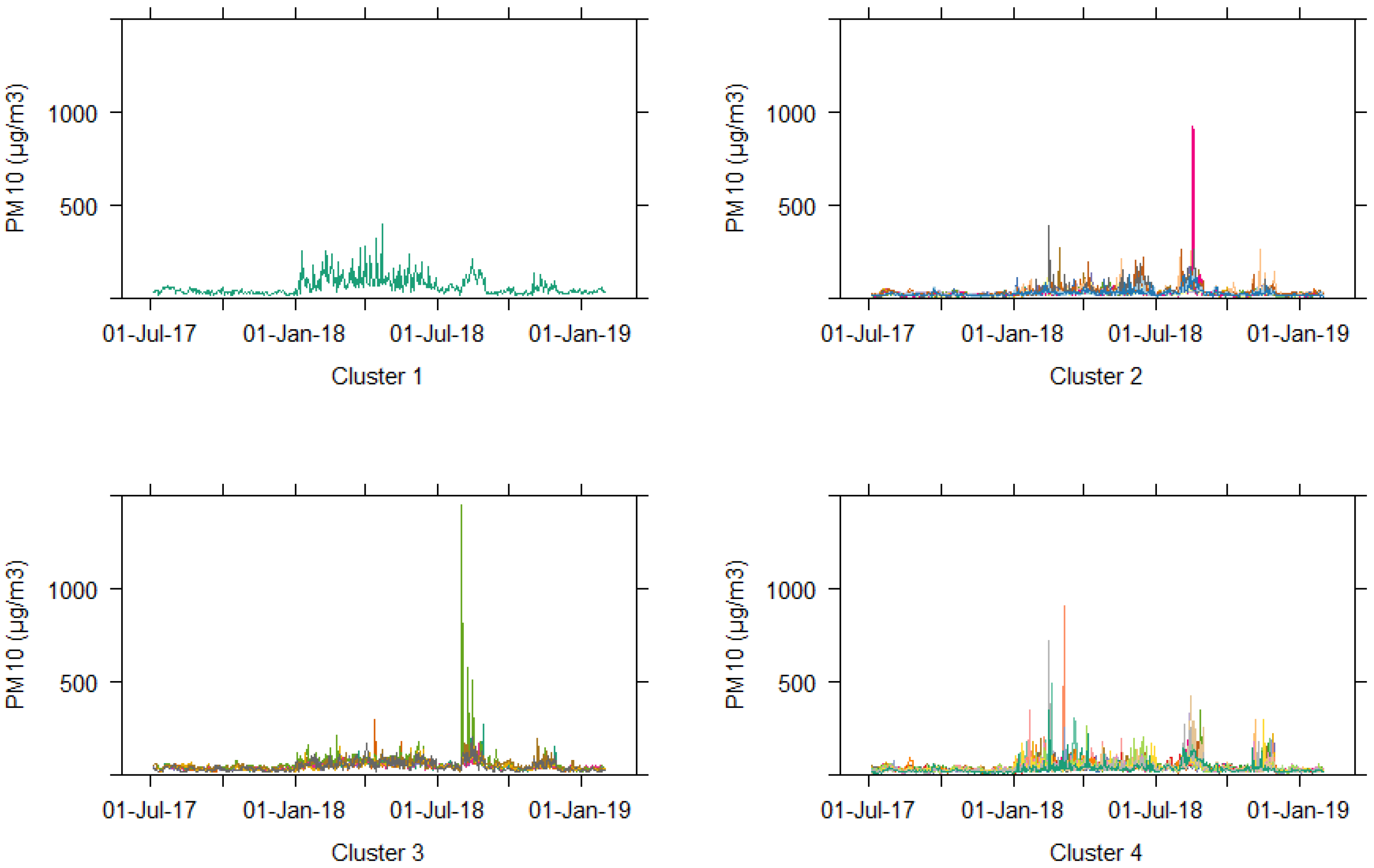
3. Results and Analysis

Four different univariate cluster analyses were performed in this study. In this context, all cluster analyses used DTW as the dissimilarity measure along with various clustering algorithms such as k-Means, PAM, hierarchical, and FKM.

In this study, hourly PM₁₀ data from 5 July 2017 until 31 January 2019 from 60 stations located in Malaysia (Figure 1), categorized as rural, urban, sub-urban, and industry areas, were obtained from the Department of Environment (DOE), Malaysia and clustered into several groups. It is essential to group the monitoring stations into clusters as each member in the respective cluster may provide homogenous information from the air quality pattern, thus, the formation of the clusters can evade redundancy [40], especially given that the cost for air quality monitoring is expensive. Information from this study may help the respective agencies in Malaysia to manage the air quality standards and the impacts of air pollutions in Malaysia.

Imputation of missing values in this study was done by applying the linear interpolation method. Many research examples on air quality time series have used the linear interpolation method for data imputation such as studies by Ottosen and Kumar [41], Yen et al. [42] and Junninen et al. [43] especially for the imputation of short gap missing values and because of the simplicity of the technique. Figure 2 shows the maximum missing values gap in hours for every station which are relatively small compared to the total length of the PM₁₀ data used.

Since the DTW is computationally expensive [44], the hourly time series data were converted into daily average and daily maximum time series data. By using the daily average time series, information on the daily cycle cannot be observed, thus resulting in the loss of information. However, because of the limitation in terms of the computational cost for clustering hourly time series, this study opted for daily average time series. This study also considered clustering of the daily maximum time series to minimize the loss of information caused by using the average daily time series. The air quality monitoring stations are clustered into four groups based on the optimal number of clusters determined by the elbow technique [45]. The methodology flowchart in this study is shown in Figure 3.

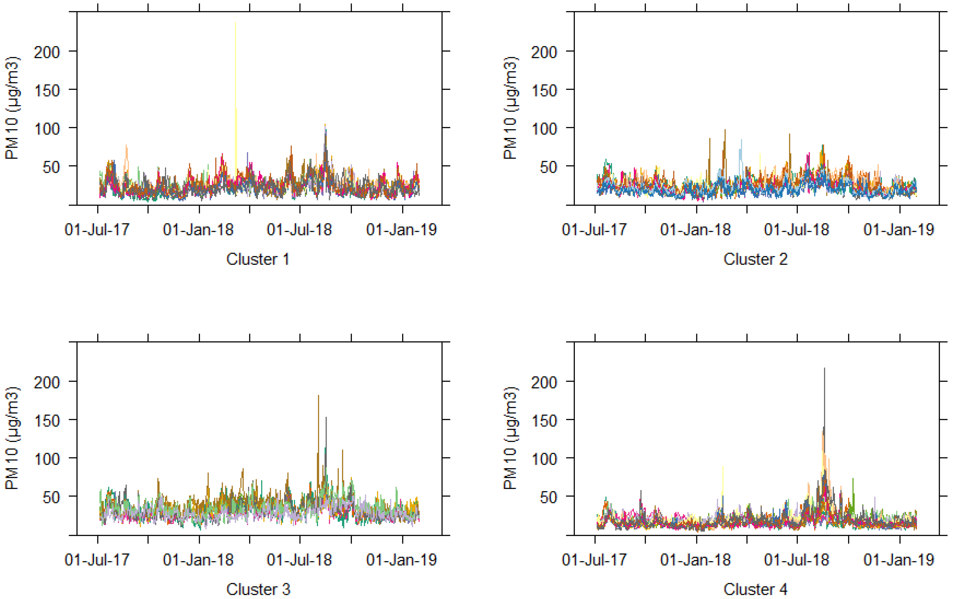
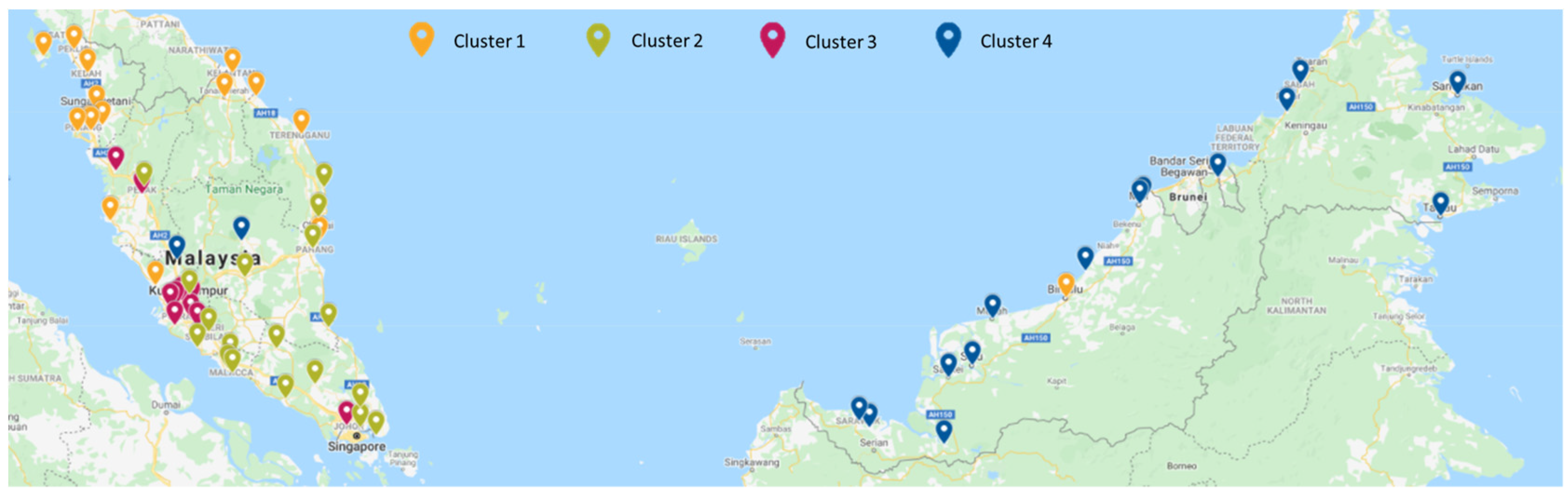
3.1. Clustering of Daily Average Data

The daily average time series of all 60 stations are used to obtain the four clusters of air quality in Malaysia. Figure 4, Figure 5, Figure 6 and Figure 7 show the daily average time series plots for the four clusters obtained based on k-Means, PAM, hierarchical, and FKM, respectively. Based on those figures, the time series plots for each cluster show similar patterns in terms of magnitudes and occurrence of extreme events. In addition, all four methods manage to distinguish dissimilarities in the time series patterns between different clusters.

Figure 8 and

Table 1. Minimum, lower quartile, median, upper quartile, and maximum (below upper fence) observations of PM₁₀ according to clusters based on four clustering algorithms for daily average data extracted from the corresponding boxplots.

Algorithms	Cluster	Minimum Observation	Lower Quartile	Median	Upper Quartile	Maximum Observation (Below Upper Fence)
DTW + k-Means	Cluster 1	6.52	20.37	25.78	32.92	51.71
	Cluster 2	4.46	16.01	20.55	26.67	42.67
	Cluster 3	6.57	25.46	31.75	39.67	60.86
	Cluster 4	4.37	12.96	15.92	20.23	31.13
DTW + PAM	Cluster 1	4.46	16.71	22.00	28.86	47.06
	Cluster 2	4.37	17.47	22.54	29.13	46.58
	Cluster 3	6.57	24.46	30.51	38.05	58.21
	Cluster 4	4.55	13.42	16.67	21.58	33.80
DTW + Hierarchical	Cluster 1	6.57	22.81	28.57	35.69	54.97
	Cluster 2	4.46	16.37	21.23	27.71	44.69
	Cluster 3	14.11	28.02	36.01	46.22	73.38
	Cluster 4	4.37	13.31	16.40	21.13	32.84
DTW + FKM	Cluster 1	6.52	19.96	25.38	32.54	51.42
	Cluster 2	5.00	16.33	20.90	26.87	42.67
	Cluster 3	6.57	25.46	31.75	39.67	60.86
	Cluster 4	4.37	13.05	16.32	21.10	33.13

show the distribution of daily average PM₁₀ time series data for each cluster. Based on the boxplots, there are differences in the daily average time series distribution between each cluster, especially in terms of the median. This is observed from the boxplots of all four algorithms except for the median of clusters 1 and 2 from the DTW with the PAM algorithm. Based on the boxplots for all algorithms used, cluster 3 consists of time series with higher daily average values of PM₁₀ compared to other clusters, indicated by the high median value. On the other hand, cluster 4 consists of time series with lower values of PM₁₀ daily average, as its median is lower than other clusters as shown in the boxplots.

Table 2. Cluster membership for PM₁₀ daily average data according to stations based on four clustering algorithms.

Station ID	Station Location	Station Category	DTW + k-Means	DTW + PAM	DTW + Hierarchical	DTW + FKM
CA01R	Kangar, PERLIS	Sub Urban	2	1	2	4
CA02K	Langkawi, KEDAH	Sub Urban	2	1	2	2
CA03K	Alor Setar, KEDAH	Sub Urban	2	1	2	2
CA04K	Sungai Petani, KEDAH	Sub Urban	2	1	2	2
CA05K	Kulim Hi-Tech, KEDAH	Industry	2	1	2	2
CA06P	Seberang Jaya, PULAU PINANG	Urban	1	1	2	1
CA07P	Seberang Perai, PULAU PINANG	Sub Urban	1	1	2	1
CA09P	Balik Pulau, PULAU PINANG	Sub Urban	2	1	2	4
CA10A	Taiping, PERAK	Sub Urban	3	3	1	3
CA11A	Tasek Ipoh, PERAK	Urban	1	2	1	1
CA12A	Pegoh Ipoh, PERAK	Sub Urban	3	3	1	3
CA13A	Seri Manjung, PERAK	Rural	1	1	2	1
CA14A	Tanjung Malim, PERAK	Sub Urban	4	4	4	4
CA15W	Batu Muda, KL WILAYAH PERSEKUTUAN	Sub Urban	1	2	1	1
CA16W	Cheras, KL WILAYAH PERSEKUTUAN	Urban	1	3	1	1
CA17W	Putrajaya, WILAYAH PERSEKUTUAN	Sub Urban	1	3	1	1
CA18B	Kuala Selangor, SELANGOR	Rural	2	1	2	1
CA19B	Petaling Jaya, SELANGOR	Sub Urban	3	3	1	3
CA20B	Shah Alam, SELANGOR	Urban	3	3	1	3
CA21B	Klang, SELANGOR	Sub Urban	3	3	3	3
CA22B	Banting, SELANGOR	Sub Urban	3	3	1	3
CA23N	Nilai, NEGERI SEMBILAN	Sub Urban	3	3	1	3
CA24N	Seremban, NEGERI SEMBILAN	Urban	2	2	2	2
CA25N	Port Dickson, NEGERI SEMBILAN	Sub Urban	2	2	2	2
CA26M	Alor Gajah, MELAKA	Rural	2	2	2	2
CA27M	Bukit Rambai, MELAKA	Sub Urban	1	2	1	1
CA28M	Bandaraya Melaka, MELAKA	Urban	2	2	2	1
CA29J	Segamat, JOHOR	Sub Urban	2	2	2	2
CA31J	Batu Pahat, JOHOR	Sub Urban	2	2	2	2
CA32J	Kluang, JOHOR	Rural	2	2	2	2
CA33J	Larkin, JOHOR	Urban	1	3	1	1
CA34J	Pasir Gudang, JOHOR	Urban	1	2	1	1
CA35J	Pengerang, JOHOR	Industry	2	2	2	2
CA36J	Kota Tinggi, JOHOR	Sub Urban	4	2	4	4
CA37C	Rompin, PAHANG	Rural	2	2	2	2
CA38C	Temerloh, PAHANG	Sub Urban	1	2	1	1
CA39C	Jerantut, PAHANG	Sub Urban	2	4	2	4
CA40C	Indera Mahkota, Kuantan, PAHANG	Sub Urban	2	2	2	2
CA41C	Balok Baru, Kuantan, PAHANG	Industry	1	1	1	1
CA42T	Kemaman, TERENGGANU	Industry	2	2	2	2
CA43T	Paka, TERENGGANU	Industry	2	2	2	4
CA44T	Kuala Terengganu, TERENGGANU	Urban	2	1	2	2
CA45T	Besut, TERENGGANU	Sub Urban	2	1	2	2
CA46D	Tanah Merah, KELANTAN	Sub Urban	1	1	2	1
CA47D	Kota Bahru, KELANTAN	Sub Urban	1	1	2	1
CA48S	Tawau, SABAH	Sub Urban	4	4	4	4
CA49S	Sandakan, SABAH	Sub Urban	4	4	4	4
CA50S	Kota Kinabalu, SABAH	Sub Urban	2	4	2	2
CA51S	Kimanis, SABAH	Industry	4	4	4	4
CA54Q	Limbang, SARAWAK	Rural	4	4	4	4
CA55Q	Permyjaya, Miri, SARAWAK	Rural	4	4	4	4
CA56Q	Miri, SARAWAK	Sub Urban	2	4	2	2
CA57Q	Samalaju, SARAWAK	Industry	2	4	4	2
CA58Q	Bintulu, SARAWAK	Sub Urban	1	1	2	1
CA59Q	Mukah, SARAWAK	Rural	4	4	4	4
CA61Q	Sibu, SARAWAK	Sub Urban	2	4	4	2
CA62Q	Sarikei, SARAWAK	Rural	4	4	4	4
CA63Q	Sri Aman, SARAWAK	Rural	4	4	4	4
CA64Q	Samarahan, SARAWAK	Rural	4	4	4	4
CA65Q	Kuching, SARAWAK	Urban	4	4	4	4

represents the cluster membership for PM₁₀ daily average data for 60 air quality stations in Malaysia based on DTW dissimilarity measures with four clustering algorithms. From the table, we can say that most stations are assigned to the same cluster for almost all algorithms. For example, stations CA24N, CA25N, CA26M, CA29J, CA31J, CA32J, CA35J, CA37C, CA40C, and CA42T are all assigned into cluster 2 for all clustering algorithms applied. Other than that, CA14A, CA48S, CA49S, CA51S, CA54Q, CA55Q, CA59Q, CA62Q, CA63Q, CA64Q, and CA65Q are all grouped into cluster 4. Besides that, k-Means and FKM produce almost similar clusters as the membership of every cluster formed by both algorithms is mostly the same. This is concurrent with the statement from Ghosh and Dubey [46], which emphasizes that FKM and k-Means produce alike clusters.

In addition, CA21B (Klang) monitoring station is a single member cluster formed based on agglomerative hierarchical clustering mainly due to the nature of the algorithm itself. It is shown in Figure 6 that Klang usually has a higher reading of PM₁₀ on a daily basis. In this context, hierarchical clustering allows a smaller number of members for the formation of clusters with a very contrary pattern, such as outlier stations. Wang et al. [47] and Mazarbhuiya et al. [48] highlight that hierarchical clustering can determine anomalous patterns in data. Meanwhile, other partitioning clustering algorithms prioritize equal size clusters [49]. Furthermore, according to Van der Laan et al. [23], PAM uses medoid as its cluster centroid, making it less sensitive to outliers and producing clusters 1 and 2 with almost identical distributions. However, this may also be influenced by the station’s geographical location, where the station might be clustered together with other nearest stations with almost similar PM₁₀ values. This is because PAM applies actual value from the time series data set as its medoid compared to k-Means and FKM, which use the average as the cluster centroid.

Table 3. Crosstable of the number of stations between clusters formed for each clustering algorithm with the stations’ location categories of the PM₁₀ daily average time series data.

Stations’ Location Categories	Clusters	DTW + k-Means	DTW + PAM	DTW + Hierarchical	DTW + FKM
Industry	1	1	2	1	1
	2	5	3	4	4
	3	0	0	0	0
	4	1	2	2	2
Rural	1	1	2	0	2
	2	4	3	5	3
	3	0	0	0	0
	4	6	6	6	6
Urban	1	5	2	5	6
	2	3	4	4	2
	3	1	3	0	1
	4	1	1	1	1
Sub-Urban	1	8	10	9	8
	2	14	8	17	11
	3	6	7	1	6
	4	4	7	5	7

shows the crosstable of the number of stations within each cluster formed for each clustering algorithm based on the stations’ location categories. It is found that almost all clusters are dominated by sub-urban categories for all clustering algorithms since the locations of the air quality stations in Malaysia are mostly from sub-urban areas.

Most of the stations in industrial areas are grouped into cluster 2 for all algorithms, while most of the stations in rural areas are dominated by cluster 4. Urban stations are mostly clustered into cluster 1 for k-Means, hierarchical, and FKM, with cluster 2 for PAM. A big part of sub-urban stations is placed in cluster 2 for k-Means, hierarchical, and FKM, with cluster 1 for PAM. Therefore, we can deduce that cluster 1 represents urban, cluster 2 represents industrial and sub-urban, while cluster 4 represents rural areas.

The locations considered as industrial areas by the DOE are mainly in less populated areas. We can say that the air quality in those areas is manageable since they are not clustered into cluster 3, which has the highest readings of the daily average of PM₁₀ as interpreted from the boxplots in Figure 8. On the other hand, some highly populated areas which are categorized as suburban and urban were clustered into cluster 3. Therefore, highly populated areas have higher PM₁₀ readings and poor quality of air. We can clearly see cluster 3 focuses on the Klang Valley area which is in the central part of Malaysia near to the capital city of Malaysia. This area is densely populated and deals with heavy traffic with a lot of passenger vehicles every day that contribute to production of significant amount of nitrogen oxides, carbon monoxide, and other pollutant.

Figure 9, Figure 10, Figure 11 and Figure 12 show that cluster 4 stations are distributed throughout East Malaysia for all algorithms applied. Meanwhile, stations in clusters 1 and 2 are mainly distributed throughout Peninsular Malaysia, and stations in cluster 3 are mainly located in the central part of Peninsular Malaysia. This result applied to all the algorithms used. In the east coast area of Peninsular Malaysia, most of the stations are clustered into cluster 2 and 4 which have lower air pollution as a result of lower PM₁₀ readings except for Balok Baru (CA41C), Kota Bahru (CA47D), and Tanah Merah (CA46D) which are grouped into cluster 1 that has higher PM₁₀ reading. Balok Baru has lower air quality due to its location to nearby Pelabuhan Kuantan and Gebeng which consist of many factories and massive industrial activities related to bauxite mining, oil and gas activity, as well as other manufacturing activities.

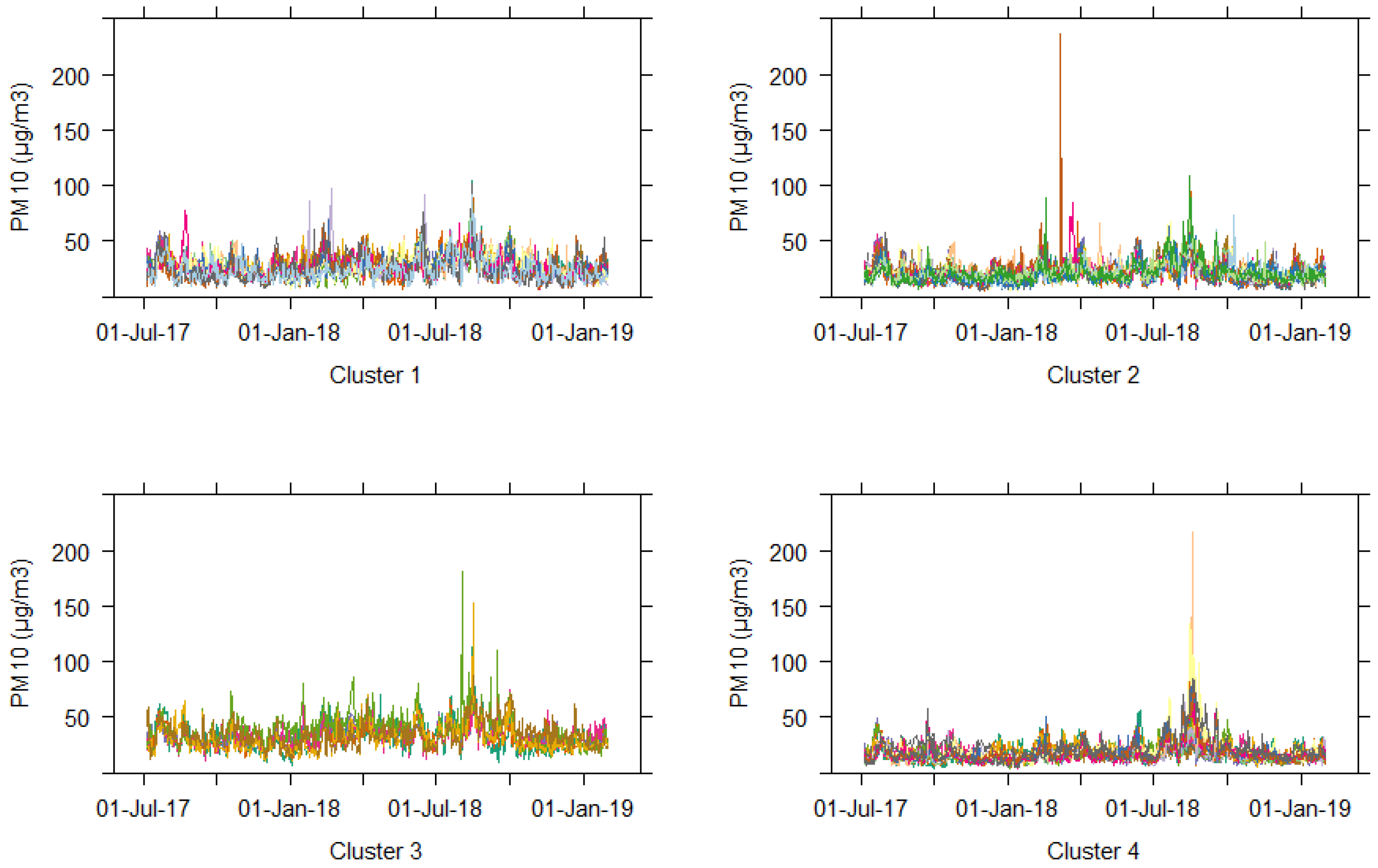
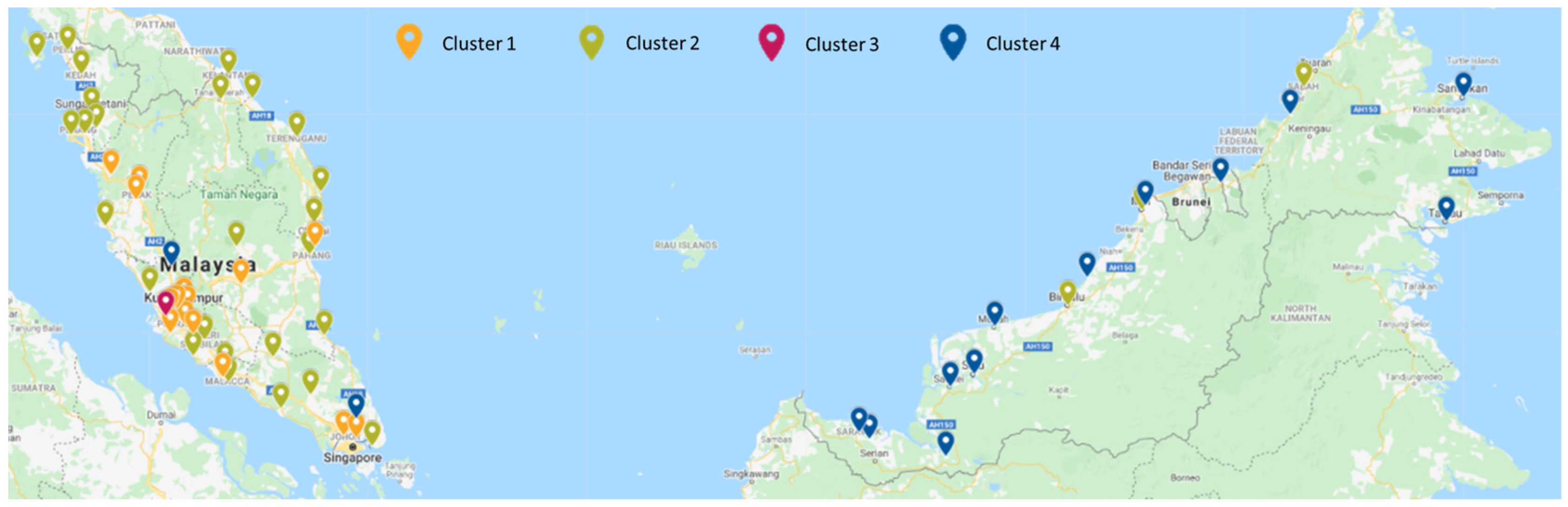
3.2. Clustering of Daily Maximum Data

Daily maximum time series are also considered in this study because it is crucial to identify stations with a high value of PM₁₀ for a shorter period. Similar to the daily average time series discussed in the previous section, the daily maximum time series of all 60 stations are used to obtain four clusters of air quality in Malaysia. Figure 13, Figure 14, Figure 15 and Figure 16 show the daily maximum time series plots for the four clusters obtained based on k-Means, PAM, hierarchical, and FKM, respectively. Cluster 1 based on PAM and hierarchical is a single member cluster of station CA10A. Meanwhile, based on k-Means and FKM, cluster 1 has two members consisting of station CA10A and CA21B. Station CA10A is located in a suburban area facing Sumatera Island and surrounded by hilly areas, which might cause higher daily maximum values than other stations. At the same time, station CA21B has a higher daily maximum, coinciding with the results in the previous section. Boxplots in Figure 17 show that the distributions of daily maximum for clusters 2, 3, and 4 are almost similar in terms of their median and variance values. The minimum, lower quartile, median, upper quartile, and maximum values from the boxplots are summarized in

Table 4. Minimum, lower quartile, median, upper quartile and maximum (below upper fence) observations of PM₁₀ according to clusters based on four clustering algorithms for daily maximum data extracted from the corresponding boxplots.

Algorithms	Cluster	Minimum Observation	Lower Quartile	Median	Upper Quartile	Maximum Observation (Below Upper Fence)
DTW + k-Means	Cluster 1	11.67	32.00	46.91	72.52	133.12
	Cluster 2	6.00	18.02	25.15	34.66	59.58
	Cluster 3	9.10	29.30	40.03	55.16	93.65
	Cluster 4	7.00	22.22	31.00	43.11	74.42
DTW + PAM	Cluster 1	11.67	29.24	43.00	74.69	142.18
	Cluster 2	6.00	17.00	23.00	31.76	53.88
	Cluster 3	11.95	31.00	41.98	57.66	97.57
	Cluster 4	7.00	23.00	31.00	42.67	72.17
DTW + Hierarchical	Cluster 1	11.67	29.24	43.00	74.69	142.18
	Cluster 2	6.00	19.00	26.33	37.00	64.00
	Cluster 3	17.00	36.00	49.00	69.87	120.01
	Cluster 4	10.00	28.00	37.00	50.24	83.37
DTW + FKM	Cluster 1	11.67	32.00	46.91	72.52	133.12
	Cluster 2	6.00	18.02	25.15	34.66	59.58
	Cluster 3	7.00	23.88	32.70	45.75	78.51
	Cluster 4	7.00	23.75	33.16	47.18	82.31

.

Table 5. Cluster membership for PM₁₀ daily maximum data according to stations based on four clustering algorithms.

Station ID	Station Location	Station Category	DTW + k-Means	DTW + PAM	DTW + Hierarchical	DTW + FKM
CA01R	Kangar, PERLIS	Sub Urban	2	2	2	2
CA02K	Langkawi, KEDAH	Sub Urban	2	4	2	2
CA03K	Alor Setar, KEDAH	Sub Urban	2	2	2	2
CA04K	Sungai Petani, KEDAH	Sub Urban	2	4	2	2
CA05K	Kulim Hi-Tech, KEDAH	Industry	4	4	2	4
CA06P	Seberang Jaya, PULAU PINANG	Urban	4	4	4	3
CA07P	Seberang Perai, PULAU PINANG	Sub Urban	4	4	4	4
CA09P	Balik Pulau, PULAU PINANG	Sub Urban	2	2	2	2
CA10A	Taiping, PERAK	Sub Urban	1	1	1	1
CA11A	Tasek Ipoh, PERAK	Urban	4	4	4	3
CA12A	Pegoh Ipoh, PERAK	Sub Urban	3	3	4	3
CA13A	Seri Manjung, PERAK	Rural	4	4	2	3
CA14A	Tanjung Malim, PERAK	Sub Urban	2	2	2	2
CA15W	Batu Muda, KL WILAYAH PERSEKUTUAN	Sub Urban	4	4	4	3
CA16W	Cheras, KL WILAYAH PERSEKUTUAN	Urban	3	3	4	3
CA17W	Putrajaya, WILAYAH PERSEKUTUAN	Sub Urban	4	4	4	3
CA18B	Kuala Selangor, SELANGOR	Rural	4	4	4	3
CA19B	Petaling Jaya, SELANGOR	Sub Urban	3	3	4	4
CA20B	Shah Alam, SELANGOR	Urban	3	3	4	3
CA21B	Klang, SELANGOR	Sub Urban	1	3	3	1
CA22B	Banting, SELANGOR	Sub Urban	3	3	4	3
CA23N	Nilai, NEGERI SEMBILAN	Sub Urban	3	3	4	4
CA24N	Seremban, NEGERI SEMBILAN	Urban	2	4	2	2
CA25N	Port Dickson, NEGERI SEMBILAN	Sub Urban	2	4	2	2
CA26M	Alor Gajah, MELAKA	Rural	2	4	2	2
CA27M	Bukit Rambai, MELAKA	Sub Urban	4	4	4	4
CA28M	Bandaraya Melaka, MELAKA	Urban	4	4	2	3
CA29J	Segamat, JOHOR	Sub Urban	2	4	2	2
CA31J	Batu Pahat, JOHOR	Sub Urban	2	4	2	2
CA32J	Kluang, JOHOR	Rural	2	4	2	2
CA33J	Larkin, JOHOR	Urban	4	4	4	3
CA34J	Pasir Gudang, JOHOR	Urban	4	4	4	4
CA35J	Pengerang, JOHOR	Industry	4	4	2	3
CA36J	Kota Tinggi, JOHOR	Sub Urban	2	2	2	2
CA37C	Rompin, PAHANG	Rural	2	4	2	2
CA38C	Temerloh, PAHANG	Sub Urban	4	4	2	3
CA39C	Jerantut, PAHANG	Sub Urban	2	2	2	2
CA40C	Indera Mahkota, Kuantan, PAHANG	Sub Urban	2	2	2	2
CA41C	Balok Baru, Kuantan, PAHANG	Industry	4	4	4	4
CA42T	Kemaman, TERENGGANU	Industry	4	4	2	4
CA43T	Paka, TERENGGANU	Industry	2	2	2	2
CA44T	Kuala Terengganu, TERENGGANU	Urban	4	4	2	3
CA45T	Besut, TERENGGANU	Sub Urban	2	4	2	2
CA46D	Tanah Merah, KELANTAN	Sub Urban	4	4	2	4
CA47D	Kota Bahru, KELANTAN	Sub Urban	3	4	2	3
CA48S	Tawau, SABAH	Sub Urban	2	2	2	2
CA49S	Sandakan, SABAH	Sub Urban	2	2	2	2
CA50S	Kota Kinabalu, SABAH	Sub Urban	4	2	2	3
CA51S	Kimanis, SABAH	Industry	2	2	2	2
CA54Q	Limbang, SARAWAK	Rural	2	2	2	2
CA55Q	Permyjaya, Miri, SARAWAK	Rural	4	2	2	3
CA56Q	Miri, SARAWAK	Sub Urban	4	2	2	4
CA57Q	Samalaju, SARAWAK	Industry	4	4	2	3
CA58Q	Bintulu, SARAWAK	Sub Urban	3	3	4	4
CA59Q	Mukah, SARAWAK	Rural	4	4	2	3
CA61Q	Sibu, SARAWAK	Sub Urban	4	4	2	4
CA62Q	Sarikei, SARAWAK	Rural	4	2	2	3
CA63Q	Sri Aman, SARAWAK	Rural	2	2	2	2
CA64Q	Samarahan, SARAWAK	Rural	2	2	2	2
CA65Q	Kuching, SARAWAK	Urban	4	4	2	4

displays the membership of all four clusters formed for PM₁₀ daily maximum of air quality time series data for each clustering algorithm applied. From the output, we can deduce that a few clustering results for all algorithms are consistent. For illustrations, CA01R, CA03K, CA09P, CA14A, CA36J, CA39C, CA40C, CA43T, CA48S, CA49S, CA51S, CA54Q, CA63Q, and CA64Q stations are all grouped into cluster 2 for all algorithms used. Apart from that, CA07P, CA27M, CA34J, and CA41C stations are clustered in the same cluster for all algorithms. However, the results from daily average data are more consistent throughout all algorithms than daily maximum data since clusters 2, 3, and 4 for daily maximum data do not have noticeable differences. The differences between both daily average and daily maximum data are due to the loss of information in the daily average data as the information on the daily cycle cannot be observed.

Table 6. Crosstable of the number of stations between clusters formed for each clustering algorithm with the stations’ location categories of the PM₁₀ daily maximum time series data.

Stations’ Location Categories	Clusters	DTW + k-Means	DTW + PAM	DTW + Hierarchical	DTW + FKM
Industry	1	0	0	0	0
	2	2	2	6	2
	3	0	0	0	2
	4	5	5	1	3
Rural	1	0	0	0	0
	2	5	5	10	6
	3	0	0	0	5
	4	6	6	1	0
Urban	1	0	0	0	0
	2	0	0	4	1
	3	2	2	0	7
	4	8	8	6	2
Sub-Urban	1	1	1	1	2
	2	11	11	21	15
	3	6	6	1	7
	4	14	14	9	8

indicates the crosstable of the number of stations between clusters formed for k-Means, PAM, agglomerative hierarchical, and FKM clustering algorithms with the stations’ location categories of the PM₁₀ daily maximum time series data. Most of the stations are grouped into clusters 4 and 2. The majority of the stations in the industrial area are grouped into cluster 4 based on k-Means, PAM, and FKM, while most of them are grouped into cluster 2 based on hierarchical algorithms. As for stations located in rural and sub-urban areas, most stations are members of cluster 4 according to k-Means and PAM, while most stations in this area are members of cluster 2 based on hierarchical and FKM algorithms. Most of the stations in urban areas are in cluster 4 based on k-Means, PAM and hierarchical, while the highest number of stations in urban areas are in cluster 3 based on the FKM algorithm. Based on this table, it can be deduced that the cluster from the daily maximum was independent of station categories.

Figure 18, Figure 19, Figure 20 and Figure 21 represent the air monitoring stations that are colored according to their clusters based on k-Means, PAM, hierarchical, and FKM, respectively, for PM₁₀ daily maximum time series data. From the plotted maps, it can be roughly seen that the distribution of cluster results is inconsistent for all algorithms. For instance, most of cluster 3 members are distributed in the Klang Valley area for k-Means, PAM, and hierarchical, while for FKM, they are distributed throughout both Peninsular and East Malaysia. Meanwhile, clusters 2 and 4 are distributed throughout Malaysia for all algorithms.

FKM and k-Means generate almost similar results for daily average but different results for daily maximum because of the nature of the algorithms themselves. According to D’Urso and Maharaj [50], the dynamic characteristic of the time series that causes the time series to belong to a certain cluster only for a certain time, makes it vague and Fuzzy k-Means is suitable to treat this vagueness as compared to traditional clustering methods such as k-Means. Mingoti and Lima [51] mentioned that Fuzzy k-Means performed better than k-Means and hierarchical clustering, as it is very stable even in the presence of overlapping and outliers.

3.3. Evaluation of Clustering

To evaluate our clustering results, a cluster validity index (CVI) was used [19].

Table 7. Rand Index values for daily average and daily maximum data for k-Means, PAM, hierarchical, and FKM.

Algorithm	Rand Index
	Daily Average	Daily Maximum
k-Means	0.6559322	0.5694915
PAM	0.7548023	0.5903955
Hierarchical	0.6423729	0.499435
FKM	0.6570621	0.580226

below shows the Rand Index values for daily average and daily maximum data for every algorithm used. From the output, we can say that PAM performs better than the other algorithms due to high values of Rand Index. FKM is the second best followed by k-Means and hierarchical.

4. Conclusions

In brief, this study implemented DTW with four different clustering algorithms, which are k-Means, PAM, hierarchical, as well as FKM on Malaysia hourly PM₁₀ time series data that had been converted into daily average and daily maximum data.

From the results for all algorithms applied, daily average data gives better, and more consistent results compared to daily maximum data. Based on the clustering results from both daily average and daily maximum time series data, it can be assumed that the clusters formed do not depend on the locations’ categories but are more influenced by the geographical characteristic of the stations’ locations. Based on the daily average time series cluster analysis, the pattern of PM₁₀ air quality data in Malaysia is significantly different for both Peninsular Malaysia and East Malaysia as they are grouped into different clusters based on all four algorithms.

All things considered, air quality condition in the central region of Peninsular Malaysia is the most worrisome due to the high population density. In contrast, the condition for the rest of Peninsular Malaysia is still manageable, and East Malaysia has the best air quality in Malaysia due to slow urbanization and development that leaves Borneo still with a lot of greens, forest, and cleaner air. However, Bintulu in Sarawak is grouped in a cluster with higher PM₁₀ values and separately from other East Malaysia air monitoring stations. This has been caused by the palm oil and crude oil refinery mills located in the surrounding area. Besides that, according to the Malaysian Department of Environment, the high PM₁₀ reading from the CA21B (Klang) monitoring station is due to the high number of factories and industrial activities. Meanwhile, the unsatisfactory quality of air in CA10A (Taiping) is highly influenced by the activities of the palm oil and carbide factories located there.

Based on the results, it was shown that the hierarchical algorithm can differentiate anomaly stations, which are dissimilar compared to other stations. However, k-Means, PAM, and FKM algorithms usually produce equal size clusters compared to the hierarchical algorithm. Furthermore, k-Means and FKM did produce almost identical clusters. As for the cluster validity index, Rand Index was used and PAM proved to perform best followed by FKM, k-Means, and hierarchical. Overall, DTW showed that it is suitable for measuring the dissimilarities for clustering time series air quality data using all four algorithms.

References

1. Afroz, R.; Hassan, M.N.; Ibrahim, N.A. Review of air pollution and health impacts in Malaysia. Environ. Res. 2003, 92, 71–77. [Google Scholar] [CrossRef]
2. Usmani, R.S.A.; Saeed, A.; Abdullahi, A.M.; Pillai, T.R.; Jhanjhi, N.; Hashem, I.A.T. Air pollution and its health impacts in Malaysia: A review. Air Qual. Atmos. Health 2020, 13, 1093–1118. [Google Scholar] [CrossRef]
3. Azmi, S.Z.; Latif, M.T.; Ismail, A.S.; Juneng, L.; Jemain, A.A. Trend and status of air quality at three different monitoring stations in the Klang Valley, Malaysia. Air Qual. Atmos. Health 2010, 3, 53–64. [Google Scholar] [CrossRef] [PubMed] [Green Version]
4. Aghabozorgi, S.; Shirkhorshidi, A.S.; Wah, T.Y. Time-series clustering–A decade review. Inf. Syst. 2015, 53, 16–38. [Google Scholar] [CrossRef]
5. D’Urso, P.; Cappelli, C.; Di Lallo, D.; Massari, R. Clustering of financial time series. Phys. A Stat. Mech. Appl. 2013, 392, 2114–2129. [Google Scholar] [CrossRef]
6. Lavin, A.; Klabjan, D. Clustering time-series energy data from smart meters. Energy Effic. 2015, 8, 681–689. [Google Scholar] [CrossRef] [Green Version]
7. Ariff, N.M.; Abu Bakar, M.A.; Mahbar, S.F.S.; Nadzir, M.S.M. Clustering of Rainfall Distribution Patterns in Peninsular Malaysia Using Time Series Clustering Method. Malays. J. Sci. 2019, 38, 84–99. [Google Scholar] [CrossRef]
8. Chandra, B.; Gupta, M.; Gupta, M.P. A multivariate time series clustering approach for crime trends prediction. In Proceedings of the 2008 IEEE International Conference on Systems, Man and Cybernetics, Singapore, 12–15 October 2008; pp. 892–896. [Google Scholar] [CrossRef]
9. Chen, Y.; Wang, L.; Li, F.; Du, B.; Choo, K.-K.R.; Hassan, H.; Qin, W. Air quality data clustering using EPLS method. Inf. Fusion 2017, 36, 225–232. [Google Scholar] [CrossRef]
10. Dogruparmak, S.C.; Keskin, G.A.; Yaman, S.; Alkan, A. Using principal component analysis and fuzzy c–means clustering for the assessment of air quality monitoring. Atmos. Pollut. Res. 2014, 5, 656–663. [Google Scholar] [CrossRef] [Green Version]
11. Stolz, T.; Huertas, M.E.; Mendoza, A. Assessment of air quality monitoring networks using an ensemble clustering method in the three major metropolitan areas of Mexico. Atmos. Pollut. Res. 2020, 11, 1271–1280. [Google Scholar] [CrossRef]
12. Dominick, D.; Juahir, H.; Latif, M.T.; Zain, S.M.; Aris, A.Z. Spatial assessment of air quality patterns in Malaysia using multivariate analysis. Atmos. Environ. 2012, 60, 172–181. [Google Scholar] [CrossRef]
13. Mutalib, S.N.S.A.; Juahir, H.; Azid, A.; Sharif, S.M.; Latif, M.T.; Aris, A.Z.; Zain, S.M.; Dominick, D. Spatial and temporal air quality pattern recognition using environmetric techniques: A case study in Malaysia. Environ. Sci. Process. Impacts 2013, 15, 1717–1728. [Google Scholar] [CrossRef]
14. Yan, R.; Liao, J.; Yang, J.; Sun, W.; Nong, M.; Li, F. Multi-hour and multi-site air quality index forecasting in Beijing using CNN, LSTM, CNN-LSTM, and spatiotemporal clustering. Expert Syst. Appl. 2021, 169, 114513. [Google Scholar] [CrossRef]
15. Alahamade, W.; Lake, I.; Reeves, C.E.; De La Iglesia, B. A multi-variate time series clustering approach based on intermediate fusion: A case study in air pollution data imputation. Neurocomputing 2021, in press. [CrossRef]
16. Anuradha, J.; Vandhana, S.; Reddi, S.I. Forecasting Air Quality in India through an Ensemble Clustering Technique. In Applied Intelligent Decision Making in Machine Learning; CRC Press: Boca Raton, FL, USA, 2020; pp. 113–136. [Google Scholar] [CrossRef]
17. Zhan, D.; Kwan, M.-P.; Zhang, W.; Yu, X.; Meng, B.; Liu, Q. The driving factors of air quality index in China. J. Clean. Prod. 2018, 197, 1342–1351. [Google Scholar] [CrossRef]
18. Qiao, Z.; Wu, F.; Xu, X.; Yang, J.; Liu, L. Mechanism of Spatiotemporal Air Quality Response to Meteorological Parameters: A National-Scale Analysis in China. Sustainability 2019, 11, 3957. [Google Scholar] [CrossRef] [Green Version]
19. Tüysüzoğlu, G.; Birant, D.; Pala, A. Majority Voting Based Multi-Task Clustering of Air Quality Monitoring Network in Turkey. Appl. Sci. 2019, 9, 1610. [Google Scholar] [CrossRef] [Green Version]
20. Cotta, H.H.A.; Reisen, V.A.; Bondon, P.; Filho, P.R.P. Identification of Redundant Air Quality Monitoring Stations using Robust Principal Component Analysis. Environ. Model. Assess. 2020, 25, 521–530. [Google Scholar] [CrossRef]
21. Alahamade, W.; Lake, I.; Reeves, C.E.; Iglesia, B.D.L. Clustering imputation for air pollution data. In Proceedings of the 15th International Conference, HAIS 2020, Gijón, Spain, 11–13 November 2020. [Google Scholar]
22. Govender, P.; Sivakumar, V. Application of k-means and hierarchical clustering techniques for analysis of air pollution: A review (1980–2019). Atmos. Pollut. Res. 2020, 11, 40–56. [Google Scholar] [CrossRef]
23. Van der Laan, M.; Pollard, K.; Bryan, J. A new partitioning around medoids algorithm. J. Stat. Comput. Simul. 2003, 73, 575–584. [Google Scholar] [CrossRef] [Green Version]
24. Łuczak, A.; Kalinowski, S. Fuzzy Clustering Methods to Identify the Epidemiological Situation and Its Changes in European Countries during COVID-19. Entropy 2022, 24, 14. [Google Scholar] [CrossRef] [PubMed]
25. Abu Bakar, M.A.; Ariff, N.M.; Jemain, A.A.; Nadzir, M.S.M. Cluster Analysis of Hourly Rainfalls Using Storm Indices in Peninsular Malaysia. J. Hydrol. Eng. 2020, 25, 05020011. [Google Scholar] [CrossRef]
26. Basu, B.; Srinivas, V.V. Regional flood frequency analysis using kernel-based fuzzy clustering approach. Water Resour. Res. 2014, 50, 3295–3316. [Google Scholar] [CrossRef]
27. Rai, P.; Singh, S. A survey of clustering techniques. Int. J. Comput. Appl. 2010, 7, 1–5. [Google Scholar] [CrossRef]
28. Sardá-Espinosa, A. Comparing time-series clustering algorithms in r using the dtwclust package. R Package Vignette 2017, 12, 41. [Google Scholar]
29. Niennattrakul, V.; Ratanamahatana, C.A. On clustering multimedia time series data using k-means and dynamic time warping. In Proceedings of the 2007 International Conference on Multimedia and Ubiquitous Engineering (MUE’07), Seoul, Korea, 26–28 April 2007. [Google Scholar]
30. Izakian, H.; Pedrycz, W.; Jamal, I. Fuzzy clustering of time series data using dynamic time warping distance. Eng. Appl. Artif. Intell. 2015, 39, 235–244. [Google Scholar] [CrossRef]
31. Huy, V.T.; Anh, D.T. An efficient implementation of anytime k-medoids clustering for time series under dynamic time warping. In Proceedings of the Seventh Symposium on Information and Communication Technology, Ho Chi Minh City, Vietnam, 8–9 December 2016; pp. 22–29. [Google Scholar] [CrossRef]
32. Łuczak, M. Hierarchical clustering of time series data with parametric derivative dynamic time warping. Expert Syst. Appl. 2016, 62, 116–130. [Google Scholar] [CrossRef]
33. Ariff, N.M.; Abu Bakar, M.A.; Zamzuri, Z.H. Academic preference based on students’ personality analysis through k-means clustering. Malays. J. Fundam. Appl. Sci. 2020, 16, 328–333. [Google Scholar] [CrossRef]
34. Maharaj, E.A.; D’Urso, P.; Caiado, J. Time Series Clustering and Classification; CRC Press: Boca Raton, FL, USA, 2019. [Google Scholar] [CrossRef]
35. Kaufman, L.; Rousseeuw, P.J. Partitioning around medoids (program pam). In Finding Groups in Data: An Introduction to Cluster Analysis; Wiley: Hoboken, NJ, USA, 1990; Volume 344, pp. 68–125. [Google Scholar]
36. Zhao, Y.; Karypis, G. Evaluation of hierarchical clustering algorithms for document datasets. In Proceedings of the Eleventh International Conference on Information and Knowledge Management, McLean, VA, USA, 4–9 November 2002. [Google Scholar]
37. Sonagara, D.; Badheka, S. Comparison of basic clustering algorithms. Int. J. Comput. Sci. Mob. Comput. 2014, 3, 58–61. [Google Scholar]
38. Rani, Y.; Rohil, H. A study of hierarchical clustering algorithm. Int. J. Inf. Comput. Technol. 2013, 3, 1225–1232. [Google Scholar]
39. Xu, D.; Tian, Y. A Comprehensive Survey of Clustering Algorithms. Ann. Data Sci. 2015, 2, 165–193. [Google Scholar] [CrossRef] [Green Version]
40. D’Urso, P.; Massari, R.; Cappelli, C.; De Giovanni, L. Autoregressive metric-based trimmed fuzzy clustering with an application to PM10 time series. Chemom. Intell. Lab. Syst. 2017, 161, 15–26. [Google Scholar] [CrossRef]
41. Ottosen, T.-B.; Kumar, P. Outlier detection and gap filling methodologies for low-cost air quality measurements. Environ. Sci. Processes Impacts 2019, 21, 701–713. [Google Scholar] [CrossRef]
42. Yen, N.Y.; Chang, J.-W.; Liao, J.-Y.; Yong, Y.-M. Analysis of interpolation algorithms for the missing values in IoT time series: A case of air quality in Taiwan. J. Supercomput. 2020, 76, 6475–6500. [Google Scholar] [CrossRef]
43. Junninen, H.; Niska, H.; Tuppurainen, K.; Ruuskanen, J.; Kolehmainen, M. Methods for imputation of missing values in air quality data sets. Atmos. Environ. 2004, 38, 2895–2907. [Google Scholar] [CrossRef]
44. Meesrikamolkul, W.; Niennattrakul, V.; Ratanamahatana, C.A. Shape-based clustering for time series data. In Proceedings of the 16th Pacific-Asia Conference, PAKDD 2012, Kuala Lumpur, Malaysia, 29 May–1 June 2012. [Google Scholar] [CrossRef]
45. Syakur, M.A.; Khotimah, B.K.; Rochman, E.M.S.; Satoto, B.D. Integration K-Means Clustering Method and Elbow Method for Identification of The Best Customer Profile Cluster. IOP Conf. Ser. Mater. Sci. Eng. 2018, 336, 012017. [Google Scholar] [CrossRef] [Green Version]
46. Ghosh, S.; Dubey, S.K. Comparative analysis of k-means and fuzzy c-means algorithms. Int. J. Adv. Comput. Sci. Appl. 2013, 4, 35–39. [Google Scholar] [CrossRef] [Green Version]
47. Wang, Y.; Qin, K.; Chen, Y.; Zhao, P. Detecting Anomalous Trajectories and Behavior Patterns Using Hierarchical Clustering from Taxi GPS Data. ISPRS Int. J. Geo-Inf. 2018, 7, 25. [Google Scholar] [CrossRef] [Green Version]
48. Mazarbhuiya, F.A.; AlZahrani, M.Y.; Georgieva, L. Anomaly detection using agglomerative hierarchical clustering algorithm. In Proceedings of the 9th iCatse Conference on Information Science and Applications, Hong Kong, China, 25–27 June 2018. [Google Scholar]
49. Reynolds, A.P.; Richards, G.; de la Iglesia, B.; Rayward-Smith, V.J. Clustering Rules: A Comparison of Partitioning and Hierarchical Clustering Algorithms. J. Math. Model. Algorithms 2006, 5, 475–504. [Google Scholar] [CrossRef]
50. D’Urso, P.; Maharaj, E.A. Autocorrelation-based fuzzy clustering of time series. Fuzzy Sets Syst. 2009, 160, 3565–3589. [Google Scholar] [CrossRef]
51. Mingoti, S.A.; Lima, J.O. Comparing SOM neural network with Fuzzy c-means, K-means and traditional hierarchical clustering algorithms. Eur. J. Oper. Res. 2006, 174, 1742–1759. [Google Scholar] [CrossRef]
Figure 1. Air quality monitoring stations according to location categories: PM10 time series data that was used in this study were collected from 60 monitoring stations in Peninsular Malaysia and East Malaysia.
Atmosphere 13 00503 g001
Figure 2. Maximum length of gaps of missing values for PM10 data from 60 air quality monitoring stations in Malaysia.
Atmosphere 13 00503 g002
Figure 3. Methodology flowchart.
Atmosphere 13 00503 g003
Figure 4. Time series plots for each cluster formed based on DTW and k-Means for daily average PM10 time series data.
Atmosphere 13 00503 g004
Figure 5. Time series plots for each cluster formed based on DTW and PAM for daily average PM10 time series data.
Atmosphere 13 00503 g005
Figure 6. Time series plots for each cluster formed based on DTW and hierarchical for daily average PM10 time series data.
Atmosphere 13 00503 g006
Figure 7. Time series plots for each cluster formed based on DTW and FKM for daily average PM10 time series data.
Atmosphere 13 00503 g007
Figure 8. Boxplots for Malaysia PM10 value (µg/m3) according to clusters based on four clustering algorithms for daily average data: (a) DTW with k-Means; (b) DTW with PAM; (c) DTW with hierarchical; (d) DTW with FKM. Lower whisker represents minimum observation, lower hinge represents lower quartile, the middle line represents median, upper hinge represents upper quartile, and upper whisker represents maximum observation.
Atmosphere 13 00503 g008
Figure 9. Air monitoring stations’ locations colored according to clusters for PM10 daily average time series data with DTW and k-Means as its clustering algorithm.
Atmosphere 13 00503 g009
Figure 10. Air monitoring stations’ locations colored according to clusters for PM10 daily average time series data with DTW and PAM as its clustering algorithm.
Atmosphere 13 00503 g010
Figure 11. Air monitoring stations’ locations colored according to clusters for PM10 daily average time series data with DTW and agglomerative hierarchical as its clustering algorithm.
Atmosphere 13 00503 g011
Figure 12. Air monitoring stations’ locations colored according to clusters for PM10 daily average time series data with DTW and FKM as its clustering algorithm.
Atmosphere 13 00503 g012
Figure 13. Time series plots for each cluster formed based on DTW and k-Means for daily maximum PM10 time series data.
Atmosphere 13 00503 g013
Figure 14. Time series plots for each cluster formed based on DTW and PAM for daily maximum PM10 time series data.
Atmosphere 13 00503 g014
Figure 15. Time series plots for each cluster formed based on DTW and hierarchical for daily maximum PM10 time series data.
Atmosphere 13 00503 g015
Figure 16. Time series plots for each cluster formed based on DTW and FKM for daily maximum PM10 time series data.
Atmosphere 13 00503 g016
Figure 17. Boxplots for Malaysia PM10 value (µg/m3) according to clusters based on four clustering algorithms for daily maximum data: (a) DTW with k-Means; (b) DTW with PAM; (c) DTW with hierarchical; (d) DTW with FKM. Lower whisker represents minimum observation, lower hinge represents lower quartile, the middle line represents median, upper hinge represents upper quartile, and upper whisker represents maximum observation.
Atmosphere 13 00503 g017
Figure 18. Air monitoring stations’ locations colored according to clusters for PM10 daily maximum time series data with DTW and k-Means as its clustering algorithm.
Atmosphere 13 00503 g018
Figure 19. Air monitoring stations’ locations colored according to clusters for PM10 daily maximum time series data with DTW and PAM as its clustering algorithm.
Atmosphere 13 00503 g019
Figure 20. Air monitoring stations’ locations colored according to clusters for PM10 daily maximum time series data with DTW and agglomerative hierarchical as its clustering algorithm.
Atmosphere 13 00503 g020
Figure 21. Air monitoring stations’ locations colored according to clusters for PM10 daily maximum time series data with DTW and FKM as its clustering algorithm.
Atmosphere 13 00503 g021