Article

Low- and Medium-Cost Sensors for Tropospheric Ozone Monitoring—Results of an Evaluation Study in Wrocław, Poland

1
Department of Air Conditioning, Heating, Gas Engineering and Air Protection, Faculty of Environmental Engineering, Wroclaw University of Science and Technology, Norwida 4/6 Str., 50-373 Wrocław, Poland
2
INSYSPOM, Krzywoustego 6-12 Str., 51-165 Wrocław, Poland
3
Department of Climatology and Atmosphere Protection, Institute of Geography and Regional Development, University of Wroclaw, Kosiby 8 Str., 51-621 Wrocław, Poland
*
Author to whom correspondence should be addressed.
Atmosphere 2022, 13(4), 542; https://doi.org/10.3390/atmos13040542
Submission received: 25 February 2022 / Revised: 24 March 2022 / Accepted: 28 March 2022 / Published: 29 March 2022
(This article belongs to the Special Issue Air Pollution, Air Quality and Human Health)

Abstract

:
The paper presents the results of a 1.5-year evaluation study of low- and medium-cost ozone sensors. The tests covered electrochemical sensors: SensoriC O3 3E 1 (City Technology) and semiconductor gas sensors: SM50 OZU (Aeroqual), SP3-61-00 (FIS) and MQ131 (Winsen). Three copies of each sensor were enclosed in a measurement box and placed near the reference analyser (MLU 400). In the case of SensoriC O3 3E 1 sensors, the R2 values for the 1-h data were above 0.90 for the first 9 months of deployment, but a performance deterioration was observed in the subsequent months (R2 ≈ 0.6), due to sensor ageing processes. High linear relationships were observed for the SM50 devices (R2 > 0.94), but some periodic data offsets were reported, making regular checking and recalibration necessary. Power-law functions were used in the case of SP3-61-00 (R2 = 0.6–0.7) and MQ131 (R2 = 0.4–0.7). Improvements in the fittings were observed for models that included temperature and relative humidity data. In the case of SP3-61-00, the R2 values increased to above 0.82, while for MQ131 they increased to above 0.86. The study also showed that the measurement uncertainty of tested sensors meets the EU Directive 2008/50/EC requirements for indicative measurements and, in some cases, even for fixed measurements.

1. Introduction

Tropospheric ozone (O3) is one of six criteria air pollutants and plays a key role in the atmospheric environment due to its ability to oxidize many trace gases and its impact on the energy budget of the troposphere. It is also one of the most important greenhouse gases as a so-called short-lived climate factor (SLCF) [1,2,3].
Surface ozone has a detrimental effect on human health [4,5], affects the cardiovascular, nervous and respiratory systems (e.g., it can aggravate lung diseases such as chronic obstructive pulmonary disease—COPD), and causes premature death, especially due to respiratory illnesses [6,7,8]. According to recent studies, in 2010 approximately 1 million premature respiratory deaths worldwide could be attributed to long-term exposure to O3 [9]. Furthermore, ozone causes damage to plants [10,11,12] and materials [13]. EEA [14] has reported that about 99% of the urban population lives in the environment, where the concentration of ozone exceeds the new WHO guideline [15].
O3 is mainly formed by complex secondary reactions of volatile organic compounds (VOCs) and nitrogen oxides (NOx) under sunlight [16,17]. The spatial variation of ozone concentration is controlled by the emission rate of precursors from anthropogenic and natural sources (e.g., biogenic VOCs) [18,19,20]. In urban areas, identifying the sensitivity of O3 formation is difficult due to complex atmospheric chemical mechanisms. Some studies reported that temporal variation of O3 production was more VOC-sensitive in the early morning and NOx-sensitive for most of the afternoon [21], while during different precursor regimes and meteorological conditions, O3 production is sensitive towards NOx [22]. In China, most urban areas are located in a VOC-sensitive or transition regime [23]. In rural areas, the availability of NOx is more important [24,25].
The rates of O3 formation also depend on favourable meteorological conditions, such as incoming solar radiation and high temperature [26,27]. Therefore, climate-change-related increases in global temperature and frequency of heatwaves could lead to elevated concentrations of ozone corresponding to threats to human health [1,28,29,30,31,32]. It should be noted that atmospheric processes of ozone formation are very complex, and therefore extensive networks of continuous measurements and appropriate models are necessary to assess exposure to this pollutant and to understand future changes.
Although spatiotemporal changes in O3 concentrations are rather regular over large distances, on the local scale, intra-urban variability of ozone precursors emission leads to a large variation in O3 levels [33]. Evaluation of these small-scale variations, which allows understanding of the mechanism of O3 formation and destruction, is extremely important to control precursor emissions and implement proper health policies [34,35]. However, conventional O3 measurement stations based on UV absorption are expensive and have relatively high power consumption, and their spatial coverage is not very dense. Due to these disadvantages, new approaches are sought and sensor technology is gaining popularity in this field [36]. Networks of sensor devices can complement traditional air-quality monitoring and improve the spatial and temporal resolution of air quality measurements [37].
Two types of O3 sensors are currently available on the market: electrochemical and metal oxide semiconductor gas sensors. The principle of operation of the electrochemical sensor is based on a chemical reaction between the target gas and the electrolyte on the surface of the working electrode. It results in a current flow that is proportional to the concentration of the gas being measured [38,39]. The operation principle of the metal oxide sensor is based on changes in the conductivity of the semiconductor material, as a function of changes in gas concentration [40]. In the case of ozone, as its concentration increases, the conductivity of the sensor decreases, and sensor responses might be measured as voltage variations on the load resistor connected in series to the sensor. Both types of sensors have been used successfully to monitor ozone concentrations in recent studies [33,38,41,42,43,44,45].
In general, the prices of O3 sensors are several orders of magnitude lower than the cost of regulatory-grade instrumentation. However, the price range of commercially available devices is wide and there is no single definition of “low-cost” or “medium-cost” sensors [46,47,48]. For this study, it was assumed that “low-cost” sensors are those that are in the range of a few tens of dollars (below USD 100). Devices that cost up to a few hundred dollars were defined as “medium-cost”. Selecting a sensor from a specific price group is an important part of creating a measurement device or monitoring network, and knowing the capabilities and limitations of such devices is crucial for both professional researchers and citizen scientists [49,50].
The purpose of this study was to examine the performance of selected O3 sensors in ambient air in Wrocław, Poland. The research was also intended to determine the suitability of the sensors for the design of a future O3 monitoring network. Four sensor models were enclosed in a measurement box and collocated with a UV-absorption analyser. The sensors were evaluated in several aspects: stability of long-term operation under changing meteorological conditions, reproducibility of sensor units, linearity of outputs and relationship to reference data, and measurement uncertainty.

2. Material and Methods

2.1. Measurement Site Description

The measurement campaign was carried out from June 2019 to December 2020 at the Meteorological Observatory of the Department of Climatology and Atmosphere Protection of the University of Wrocław (8 Kosiby Street, Wrocław, Poland). The observatory is located in the eastern district of Wrocław, on a detached housing estate, near allotments and a large city park. There are no industrial facilities in its vicinity and the distance to the nearest roads with medium traffic intensity is around 120 m. The sampling systems of the ozone measuring devices were mounted on a measurement platform, at a height of approximately 15 m above the ground level. This altitude is higher than that for typical ozone samplers used in Poland (2.5–4 m), but due to lower sensitivity to any possible local emissions it is more suitable for atmospheric measurements.

2.2. Reference Ozone Data

Ozone concentration measurements from the MLU 400 analyser (MLU Messtechnik für Luft und Umwelt, Essen, Germany) were used as reference values. The principle of operation of that instrument is based on ultraviolet absorption, and the device meets the ISO 13964:1998 standard. The instrument service was performed annually, and the calibration procedure was executed automatically by the device. Measurement data (1 min) were stored in the external database. Furthermore, meteorological variables (temperature, relative humidity, sum of incoming solar radiation) were measured at the observatory according to WMO procedures.

2.3. O3 Sensors and Measurement Setup

Sensors with different operating principles and belonging to different price ranges were selected for the study. From the low-cost sensor group, the following were used: SP3-61-00 (Nissha FIS Inc., Osaka, Japan) and MQ131 (Zhengzhou Winsen Electronics Technology Co., Ltd., Zhengzhou, China). These sensors were chosen for testing because their operation in ambient air has not been reported in detail in the literature so far. FIS sensor tests were carried out only for the older version of this device, namely the SP-61 sensor, under laboratory conditions [51] and in a field study lasting a few weeks [52]. Regarding the Winsen MQ131 sensor, its evaluation was less than 2.5 days [53].
Both devices belong to the group of semiconductor gas sensors. The SP3-61-00 sensor contains a sensing material in the form of a thin film of indium/tin oxide (ITO) formed on the alumina substrate. The heater, in the form of a thick film of ruthenium oxide, is printed on the reverse. This sensing element also contains gold electrodes and lead wires and is placed in tubular housing (h = 13 mm, φ = 14 mm). According to the technical specification, the measurement range is about 0.025–0.6 ppm. The MQ131 sensor has a similar design, but the sensitive layer is made of tungsten trioxide, applied to a ceramic tube. The complete detection element is enclosed in a plastic cap (h = 12 mm, φ = 16 mm). The detection range is approximately 0.01–1 ppm.
Sensors were purchased in 2019 at a cost of approximately USD 20 per device. In this research, three copies of each sensor model were used and connected to specially designed PCB boards equipped with microcontrollers. The designed circuits allowed the sensors to be powered and the measurement signals (volts) to be transmitted as digital values.
Another device tested, from the category of gas-sensitive semiconductor sensors, was SM50 by Aeroqual Ltd. (Auckland, New Zealand). In this research, an OZU module with a range of 0–0.15 ppm was used. Unlike the previously described sensors, this device fell into the medium-cost group—the purchase cost in 2019 was about USD 400.
The sensing element is made of tungsten trioxide, just as for MQ131, but the SM50 is a more developed measurement device consisting of multiple components mounted on a PCB board (60 mm × 75 mm). The sensor housing is a cylindrical plastic enclosure (h ≈ 15 mm, φ ≈ 16 mm) with an inlet filter and an outlet beneath the sensor. The characteristic feature of this device is a micro fan mounted on the underside, which allows the flow rate to be modulated. According to the manufacturer, the use of this procedure in conjunction with temperature modulation makes it possible to obtain adequate instrument precision and stability. The algorithms implemented reduce small baseline drifts and interfering signals (e.g., due to water vapour).
The SM50 is factory calibrated and the outputs can be analogue or digital. Aeroqual devices have been used in many studies, showing good agreement with reference instruments [54,55,56,57] and demonstrating usefulness in air-quality monitoring [33,44,45,58]. However, none of the studies that were conducted lasted more than 12 months and were carried out under very harsh meteorological conditions. For this measurement campaign, three units of this sensor were used.
The last of the devices tested was the SensoriC O3 3E 1 by City Technology (Portsmouth, Great Britain/sensors designed and manufactured in Bonn, Germany). This device is an electrochemical three-electrode sensor cell with an organic electrolyte. The purchase cost of such a sensor was about USD 400 and, for this reason, it was also classified as a medium-cost device. The measuring range of the O3 3E 1 sensor is 0–1 ppm. The sensor cover has a diameter of 15.6 mm and is approximately 14.5 mm high (“MINI” version of the enclosure). This cell is mounted on a PCB transmitter board (~25 mm × 44.5 mm) with a 4–20 mA output. The PCB also incorporates an onboard temperature compensation.
This sensor module was selected for this study because its operation has been little reported in the literature. However, it showed good performance in both laboratory [59] and five-month field studies [60]. As with previous sensors, three units of SensoriC sensor were used in this study. The short characteristics of all devices tested are shown in Table 1.
All O3 sensors were examined using a set-up developed for the testing of PM2.5 sensors [61], which ensured similar measurement conditions for the devices tested. Sensors were placed inside a handmade PVC box with a rainproof lid, where outside air was drawn through openings in one of the walls and exhausted by fans mounted on the opposite wall. Sensor measurement circuits were attached to PVC plates perpendicular to the bottom of the box. The system contained power supplies and a microcomputer that sent the measurement results to a database. Multiport USB hubs and MODBUS modules were used to transmit data from the sensors to the microcomputer. The system also included a probe with temperature and humidity sensors to monitor the conditions inside the box. The box was attached to the measurement platform at a distance of approximately 1.5 m from the inlet of the reference analyser.

3. Data Analysis

3.1. Data Preparation

Data from 13 June 2019 to the end of 2020 were taken for this analysis. In the case of the MLU 400 analyser, a preliminary data selection was performed. First of all, all data related to maintenance and service works were removed. Then, a comparison was made with data from the national monitoring station and outlier signals were excluded.
The signals from all devices were then averaged hourly, considering datasets with at least 75% completeness. The choice of hourly averaging was dictated by the possibility of comparing such data with data from national monitoring stations and calculating 8 h running averages, which was necessary to test the equivalence of sensor measurements data (Section 3.4 and Section 4.5).

3.2. Reproducibility between Units

The reproducibility of sensor units (intramodel variability) is an important feature regarding the calibration of such devices. Sensors with high reproducibility do not have to be calibrated individually, and calibration factors from one unit could be used for others without significant loss of accuracy.
To investigate the general relationships between the sensors, Pearson’s correlation coefficient was first used. Then, the reproducibility of the sensors was evaluated by visualising the dispersion of the measurement data. For this purpose, the scatterplots of sensors outputs versus the averaged data from all units were plotted.

3.3. Relationship between O3 Sensors and Reference Analyser

Models for sensor calibration were developed assuming MLU 400 analyser hourly data as response variables and sensor signals as predictors. Reference data were expressed as µg/m3, but sensor signals were collected as µA (SensoriC O3 3E 1), ppm (Aeroqual SM50) and V (FIS SP3-61-00 and Winsen MQ131) and used in that form in calibration functions.
Based on the manufacturer’s declarations, linear models for medium-cost sensors (SensoriC by City Technology and SM50 by Aeroqual) were assumed. In the case of low-cost devices (FIS and Winsen sensors), the conductivity changes due to changes in ozone concentration are non-linear and such models were considered for them.
An additional approach to determining the calibration equations was to use multiple regression with environmental factors such as temperature and relative humidity. Such factors may influence sensor performance, and their inclusion in calibration models may be beneficial [62,63]. The goodness of fit of all models was evaluated using the coefficient of determination value (R2).

3.4. Attempts to Test the Equivalence of Sensor Measurements

The sensor performance and quality of the calibration models were also evaluated in terms of meeting the data quality objectives (DQO) of the European Air Quality Directive 2008/50/EC [64]. The EU Directive specifies the requirements to be met by fixed regulatory monitoring stations but also permits the use of new measurement methods as long as they demonstrate equivalence with reference methods. One of the factors to check is the measurement uncertainty, and for ozone this must not exceed 15%. The Directive also allows for supplementing fixed measurements with so-called indicative measurements. The uncertainty of such a method of ozone concentration reporting should not exceed 30%.
Equivalence tests were performed according to the Guide to the Demonstration of Equivalence of Ambient Air Monitoring Methods by the EC Working Group [65]. The procedure is based on the appliance of orthogonal regression and the calculation of the expanded relative uncertainty (with the coverage factor k = 2) at a limit value. In the case of ozone, the Directive sets a target value of 120 µg/m3 for a maximum daily 8 h mean concentration.

4. Results and Discussion

4.1. Long-Term Sensor Performance

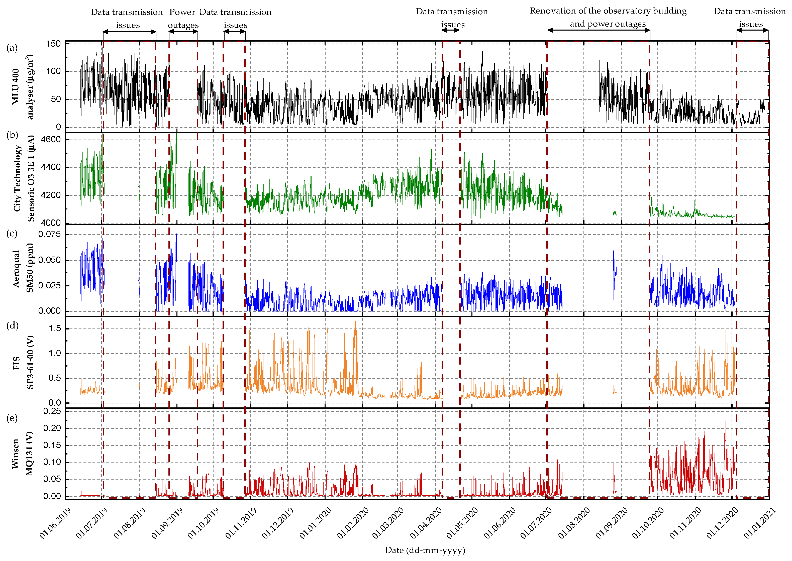
4.1.1. Evaluation of Operation Stability

Figure 1 presents the results of O3 measurements over a period of almost 1.5 years. For the sake of clarity, the outputs of only one unit of each sensor model were plotted. As can be seen, there were several issues during the measurement campaign that caused some data to be missing. Generally, data gaps occurred due to power outages or data transmission problems. In the case of the sensor measurement box, the system had to be reset in a few cases to restore data transfer. A major interruption in the measurements occurred in July and August 2020, when the observatory building was being renovated and the measurement instruments were not continuously powered. The percentage of data missing from the reference analyser was approximately 13% and for the sensor test system it was more than 30%. However, it should be noted that this situation was not related to the sensors themselves, but to the external factors mentioned above.
At the beginning of the measurement session, some malfunctions occurred with one copy of Winsen MQ131 (unit No. 1), caused by a too-loose connection to the USB hub. More serious functional problems were observed with the SensoriC O3 3E 1 sensors after about 13 months of operation. The signals from these sensors had very low values and were poorly correlated with the reference measurements. The reason for this was most likely due to sensor ageing, which is described in more detail in Section 4.3.1.

4.1.2. Meteorological Conditions and Ozone Concentrations during the Study

The study was carried out under various conditions, both in terms of ozone concentrations and meteorological variables. The air temperature recorded at the meteorological observatory ranged from −7 °C to +36 °C, and the relative humidity ranged from 10 to 100%. The highest concentration of ozone in summer reached a value greater than 140 µg/m3 while in winter it was less than 50 µg/m3. The days with the highest concentrations of ozone occurred during heatwave periods characterised by high solar radiation rates and air temperatures above 25–30 °C (Table S1 in the Supplementary Materials). Due to the heat generated by the electronics components, the temperature inside the measuring box was slightly higher and ranged from −4 °C to +37 °C (2 °C higher on average), and the relative humidity was in the range 28%–94%. However, it should be noted that the recorded high humidity conditions were at the upper limit of the operating conditions of these sensors. In addition, the sensors and electronics were also operating at sub-zero temperatures, which could affect their long-term performance.
The range of O3 concentrations registered throughout the test period with the reference analyser was 0.6–144 µg/m3. O3 concentrations were significantly positively correlated with temperature (r ≈ 0.69) and highly negatively correlated with relative humidity (r ≈ −0.80). Ozone formation was observed on warm and sunny days, especially during summer. The highest values were recorded in 2019 in June, July and August, and in 2020 in May and August. The signals from the SensoriC O3 3E 1 and SM50 sensors well tracked the reference values. The general correlation coefficients for the entire study period were in the range of 0.82–0.89 (Table 2).
The correlations for the low-cost sensors had a different character. Firstly, the raw signals measured in volts were negatively correlated with the reference values, which was due to the measurement circuit used. Secondly, the correlation coefficient values were significantly lower (level of −0.5/−0.6), due to the non-linearity in their responses. Considering the described behaviour of the sensors, calibration models were made using non-linear functions.

4.2. Reproducibility between Units

Figure S1 in the Supplementary Materials presents the correlations between all units of the sensors tested. Within a given sensor model, the highest Pearson’s correlation coefficient values were obtained for SensoriC O3 3E 1 units (r = 0.991–0.998) and Aeroqual SM50 devices (r = 0.980–0.992). Very high collinearity between units was also observed for the FIS SP3-61-00 sensor—the correlation coefficient was at the level of 0.98. For the Winsen MQ131 sensor, only units No. 2 and No. 3 were strongly correlated with each other (r= 0.975), and unit No. 1 had significantly different performance: the correlation coefficient between units 1 and 2 was 0.740 and for units 1 and 3 it was 0.666.
Figure 2 presents scatterplots of signals from sensor units versus the mean values of their 1 h averaged data. The best reproducibility between units was observed for SM50 sensors (Figure 2b). Those medium-cost sensors were calibrated by the manufacturer in the same manner, and their outputs were practically identical. The results shown are generally consistent with those of the literature: Moltchanov et al. [44] reported a high consistency of six SM50 sensors deployed in multi-sensor miniature nodes for air-quality measurements (correlations between nodes were in the range 0.92–0.99), and Jiao et al. [66] reported correlations at the level of 0.85–0.94 for SM50 sensors mounted in the field-testing device and the measurement network node.
High reproducibility was also observed for SensoriC O3 3E 1 (Figure 2a), however, for only two copies of that device. The outputs for unit No. 1 were significantly lower than for the others, although it was strongly linearly correlated with them. Similar observations regarding the slightly different performance of such sensors can be found in the literature: Spinelle et al. [60] reported that two copies of City Technology O3 3E 1F sensors operated similarly during field calibration, even if some variation could be observed.
The raw data from the low-cost sensors were characterised by a greater scatter. In the case of FIS SP3-61-00 (Figure 2c), there was a considerable agreement between the signals from units 2 and 3. Only the outputs from unit no. 1 deviated from the others, although they were strongly linearly correlated with them.
The largest discrepancy in the data was observed for the Winsen MQ131 sensor (Figure 2d). In this case, units No. 2 and No. 3 were highly correlated, although their signals did not completely overlap. A significant difference in responses was observed for unit No. 1. One reason for this may be the problems with this unit observed at the beginning of the measurement campaign. It is likely that the sensor was not properly powered and, due to the necessary resetting of the circuit, it was not able to warm up properly. The warm-up phase is required for semiconductor gas sensors to achieve chemical equilibrium with the atmosphere after they are turned on [40]. Therefore, an adequate and consistent sensor preparation time is essential before application in a monitoring network.

4.3. Relationship between O3 Sensors and Reference Analyser

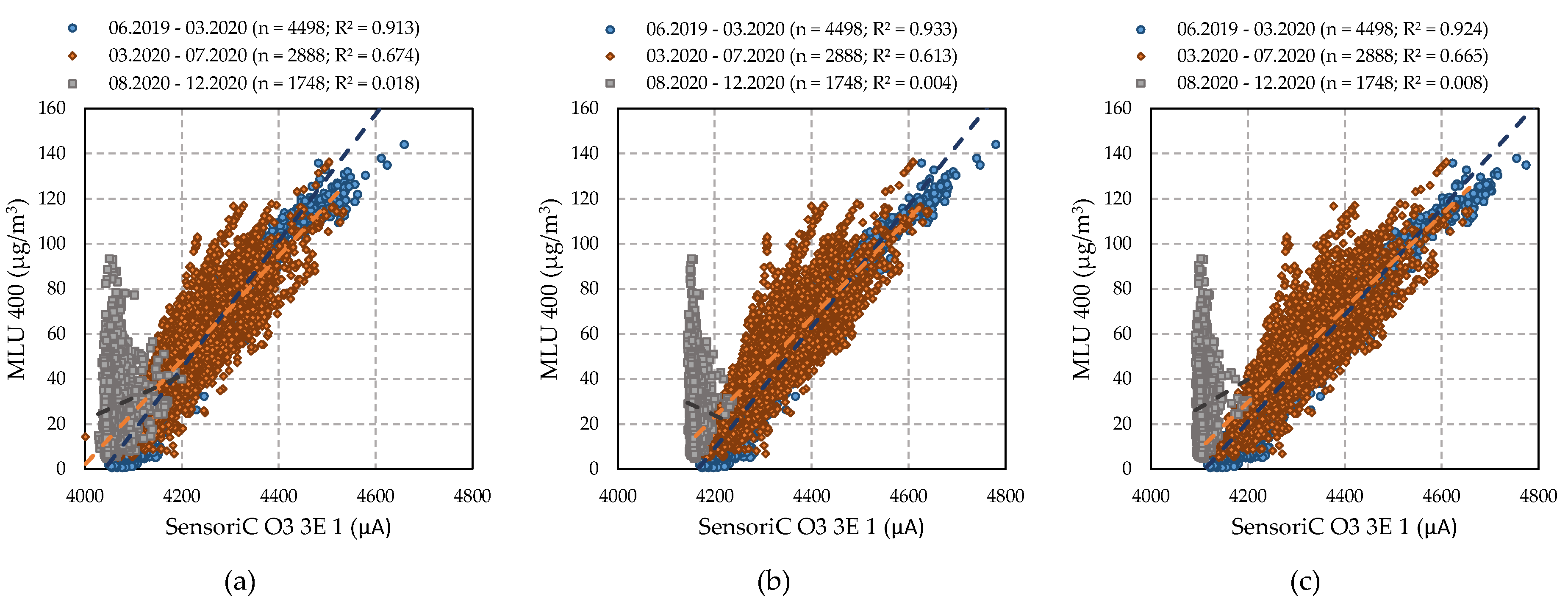
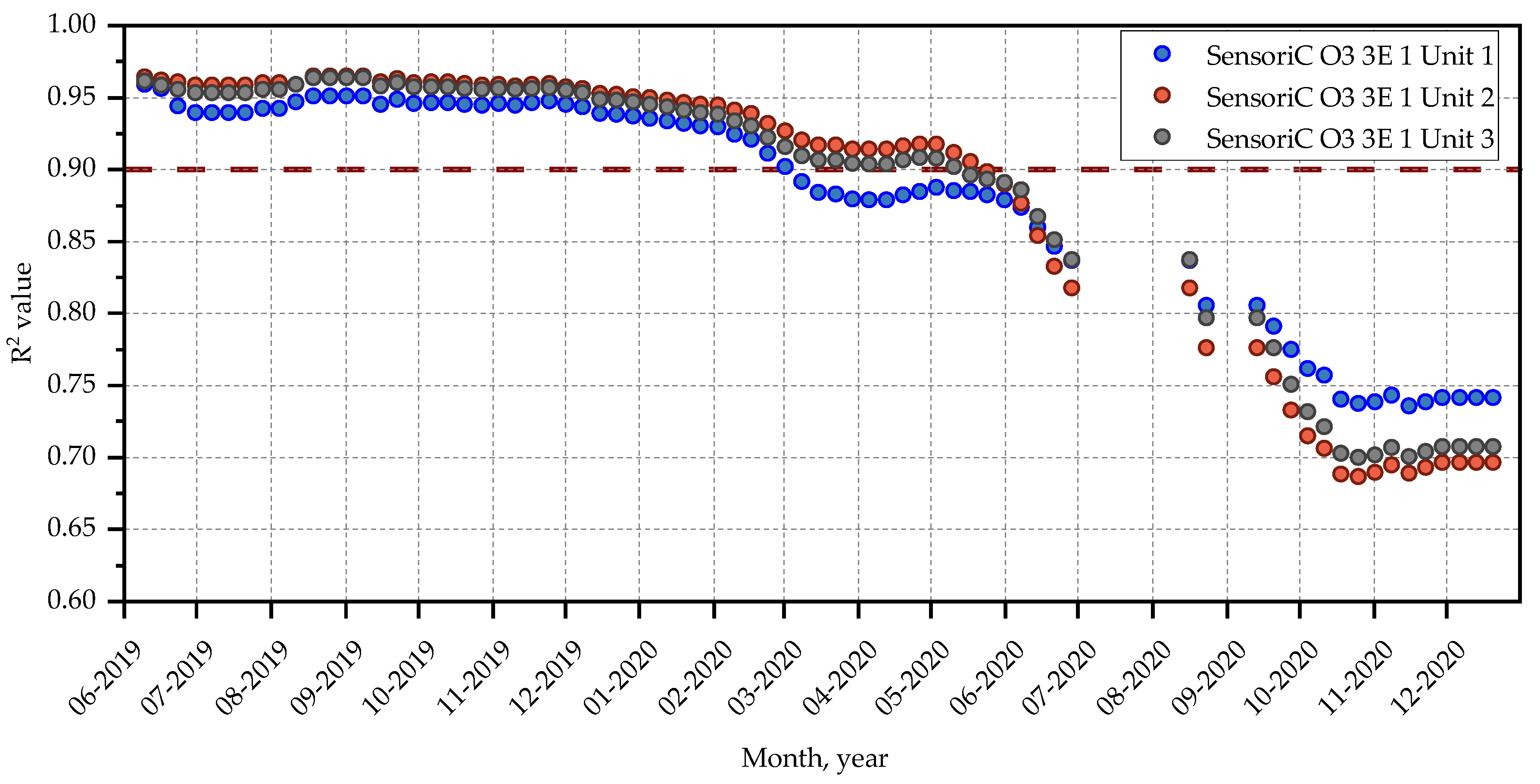
4.3.1. Performance of SensoriC O3 3E 1 Sensors (City Technology)

Figure 3 presents the results of the linear regression fittings between the O3 reference analyser and the SensoriC O3 3E 1 units. Linear models were computed for different data sets due to observed changes in sensor characteristics, as presented in Figure 4. In the case of units No. 2 and No. 3, R2 values exceeding 0.95 were obtained up to about 6 months of operation (December 2019). The results for sensor No. 1 were slightly lower—R2 was at the level of 0.93/0.94.
After 6 months of operation, the obtained R2 values decreased slightly, but were at levels greater than 0.9 for all sensors. After approximately 9 months of operation (March 2020), a significantly larger scatter of measurement data was observed (the second dataset in Figure 3), resulting in a further decrease in the R2 values. From 9 to 11 months of operation (March 2020–May 2020), R2 for units No. 1 and 2 was still above 0.9, but for unit No. 1 it dropped to ~0.88. After this time, the quality of the fits of the models decreased significantly to the level of 0.82/0.83 at the end of the 13th month of the survey (July 2020).
In the last part of the study, after a break due to the renovation of the observatory, the signals from all SensoriC units were significantly lower than those previously recorded (as can be seen in Figure 1b) and were weakly correlated with the reference data (the third dataset in Figure 3). The observed changes in the functioning of SensoriC sensors were very likely related to the ageing processes. According to the sensor datasheet, the sensor life expectancy should be no less than 18 months, but in this study, the proper operation of the sensor was observed only for a period of about 12 months. Generally, for electrochemical sensors, ageing is associated with evaporation or dilution of the electrolyte, which occurs over time [67]. However, such processes can be accelerated when the sensors are operated under adverse conditions, such as high humidity or sub-zero temperatures. Conditions such as these were encountered in this study and may have led to shorter sensor lifetimes.
The general agreement between the sensor data from SensoriC O3 3E 1 and the reference data was good. The R2 coefficients, determined for a dataset that covered 12 months of correct operation, were at the level of 0.88/0.89. Spinelle et al. [60] reported somewhat lower results for two units of SensoriC devices. For the 2 week calibration period, the R2 values were equal to 0.845 and 0.878, while for the subsequent 5 month validation period they were 0.667 and 0.813. The authors noted that the strength of the relationship between measurement devices weakened over time. This kind of behaviour could also be due to the ageing processes of the sensors.

4.3.2. Performance of SM50 OZU Sensors (Aeroqual)

Linear models of the relationship between the SM50 sensor units and the MLU 400 analyser are presented in Figure 5. As can be noticed, the Aeroqual data were characterised by high variation due to periodic offsets. For all units of SM50, it was possible to distinguish three groups of data for the following time ranges: (1) June 2019–October 2019, (2) October 2019–August 2020 and (3) August 2020–December 2020. The models for each dataset had significantly different slopes and intercepts, but in each case, they were characterised by high linearity and R2 values that exceeded 0.94.
Changes in measurement characteristics were associated with periodic shutdowns and resets of the measurement box (described in Section 4.1). As reported by Williams et al. [68], Aeroqual ozone sensors use a combination of temperature steps and air-flow-rate steps to continually reset and re-zero the sensor. In addition, when turned on, the sensor goes into a warm-up mode to burn off contaminants from the sensor. Presumably, in the case of this study, the algorithm implemented in the device’s microcontroller may have made changes to the calibration coefficients after a period of no power. The occurrences of such offsets were also mentioned in the works of Moltchanov et al. [44] and DeWitt et al. [69]. The cited authors pointed out that changes in Aeroqual sensor measurement characteristics significantly complicate O3 monitoring and suggested performing frequent calibration or data examination. Considering the results of this study, such actions should be taken at least after periods of sensor power loss. However, such actions can only be performed if the sensor is close to the reference station or if the device can be moved to such a location periodically, or by using the so-called chain calibration in the case of a distributed sensor network [70].
Overall, during periods of stable operation, the agreement between the hourly data of the SM50 OZU modules and the reference data was high. Similar observations can be found in the study by Lin et al. [55], where R2 was at the level of 0.91, and in the study by Masey et al. [56], where linear models created for different periods of operation had R2 values from 0.85 to 0.99.

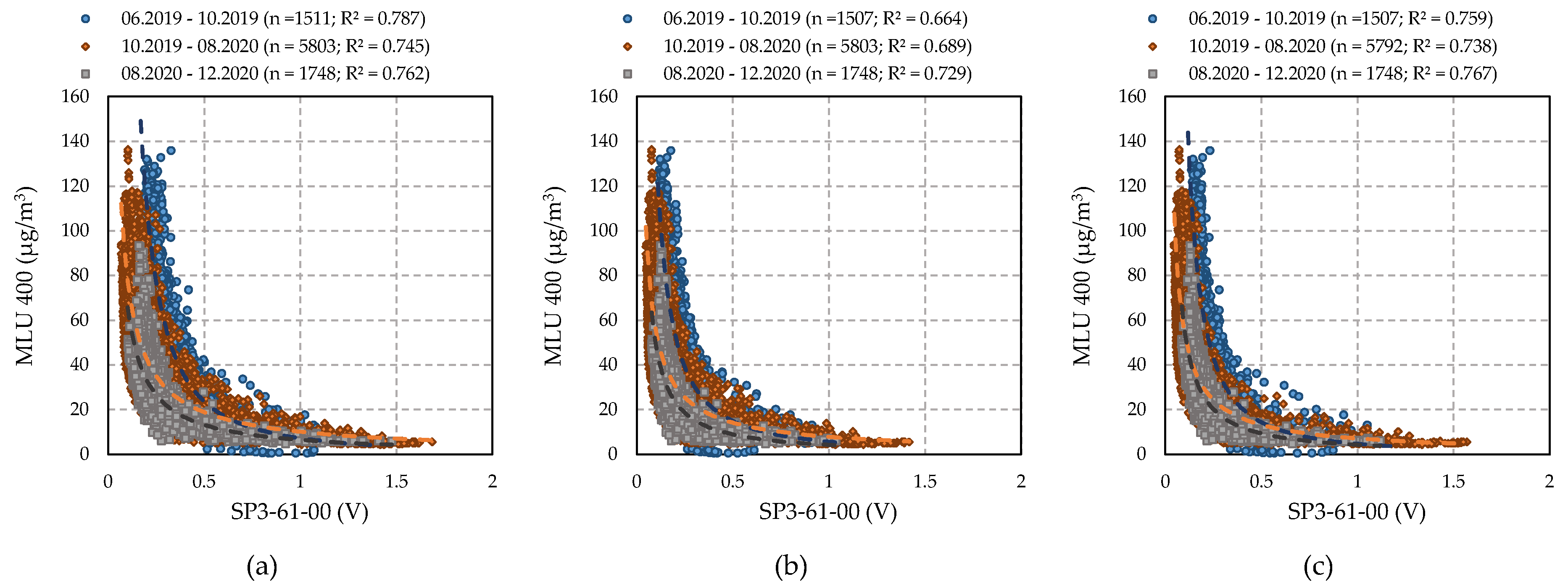
4.3.3. Performance of SP3-61-00 Sensors (FIS)

Due to the non-linearity of the FIS sensor response, power-law models were adopted for the calculations. Figure S2 in the Supplementary Materials presents the calibration models for the data set from the entire study period. The overall quality of fit was moderate: the R2 values were equal to 0.626 for unit No. 1, 0.602 for unit No. 2, and 0.630 for unit No. 3.
Given a relatively large scatter in the data and the problems observed in the cases described above, the dataset was divided into smaller sets associated with periods of continuous sensor operation (as described in Section 4.3.2). The resulting models are shown in Figure 6. In this approach, an improvement in fittings was obtained for all sub-periods: the values of R2 were in the range 0.738–0.787 for units No. 1 and No. 3, and 0.664–0.729 for unit No. 2. The distribution of the data and the calibration functions developed were quite similar for the second (October 2019–August 2020) and third (August 2020–December 2020) periods considered. Notable differences in the models were present for the initial study period (June 2019–October 2019).
It should be noted that this low-cost sensor was not equipped with any condition stabilisation system (such as flow and temperature modulation in SM50), which may have resulted in more dispersed data and changes in the output signal after the device resets.

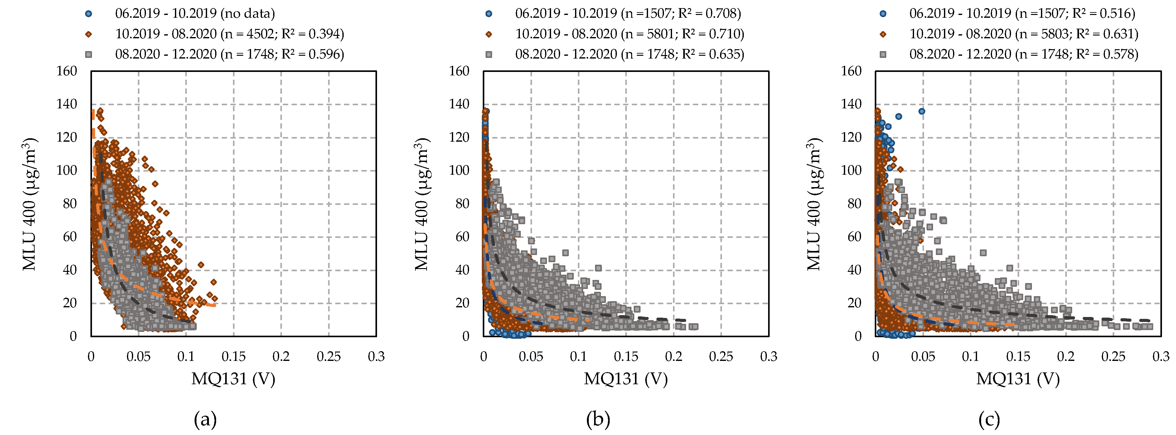
4.3.4. Performance of MQ131 Sensors (Winsen)

Similar to the FIS SP3-61-00 sensor, power-law calibration functions were used for the Winsen MQ131 sensor. The quality of the fittings for data from the entire measurement campaign is shown in Figure S3 in the Supplementary Materials. The signals from the Winsen sensors had the largest data scatter of all the devices tested. The R2 values for individual units varied widely and were equal: 0.661 for unit No. 2, 0.551 for unit No. 3, and only 0.487 for unit No. 1.
To test for changes in sensor behaviour over a long-term deployment, the dataset was divided into smaller sets, as in the previous cases. The results for the three considered time ranges are presented in Figure 7. The quality of the fit in the shorter sub-periods varied greatly depending on the particular unit. A somewhat greater improvement was observed for unit No. 2, but only in the case of the first two time periods, where the distribution of the data and the quality of the calibration functions were quite similar (R2 = 0.708 and 0.710). Data from the last measurement period were characterised by greater scatter and R2 at the level of 0.635.
In the case of unit No. 3, fittings with slightly higher R2 were achieved for the second (R2 = 0.631) and third (R2 = 0.578) periods. On the other hand, the fit was worse (R2 = 0.516) for the first period.
Problems in the functioning of unit No. 1 at the beginning of the study resulted in poor fitting quality during the second study period (R2 = 0.394). However, a smaller dispersion of the data and better fit results were achieved at the end of the study (R2 = 0.596).

4.3.5. Influence of Environmental Factors on Sensors Calibration

Tables S2–S5 in the Supplementary Materials present R2 values for calibration functions incorporating additional parameters: temperature and humidity. Data from the inside of the measurement box were used on the assumption that these parameters reflect the properties of the air in the immediate vicinity of each sensor. Calculations were made for individual measurement periods and, in some cases, for the entire study period.
For the electrochemical sensor SensoriC O3 3E 1 (Table S2), the results depended on the time period considered. For the initial 9 month period of operation, when the sensor performance was very high (R2 above 0.9 for all units), the addition of the new variables did not result in a noticeable improvement in the fit quality. Including temperature in the models raised R2 by only 0.003, and no improvement was seen with the addition of RH. On the other hand, in the second measurement period, when deterioration in sensor performance was observed, the addition of environmental parameters was beneficial. For models that additionally included only RH, the R2 values increased by 0.02 on average. When the temperature was included, R2 increased by 0.175 on average (from an average value of 0.651 to 0.826). The best results were achieved when both factors considered were included in the modelling: the increase in R2 was at the level of 0.19 and the final R2 was at the level of 0.840.
The results obtained are somewhat consistent with those reported by Spinelle et al. [59,60], who showed minor effects of temperature and humidity on the performance of the SensoriC sensors. However, these tests were conducted under laboratory conditions or as field campaigns for no more than 6 months, when sensor ageing processes may not have been noticeable. The effect of temperature on sensor performance should also be partially compensated for by the built-in algorithm. However, at a later stage of operation, as the sensor ages, this algorithm is probably no longer very effective.
As reported by Pang et al. [38], significant changes in signals and the performance of electrochemical sensors can occur with rapid variations in RH, and if the environmental RH slowly varies, the sensor performance should be relatively consistent. The issue of the influence of temperature and RH on the functioning of electrochemical sensors was also raised by Margaritis et al. [63]. The results of their investigation showed the benefits of including these parameters in calibration models and similar conclusions can be drawn in this study, especially for the long-term operation of the sensors.
Table S3 presents the results for Aeroqual SM50 sensors. In general, the addition of environmental parameters to the calibration models did not significantly improve their quality. Small increases in R2 values were observed only for models in the second and third test intervals and reached on average 0.002 when RH was included and 0.010 for temperature. For models that included both parameters, the increase in R2 was at the level of 0.011. The lack of apparent improvement in the R2 values for linear models with temperature and RH was also described by Jiao et al. [66]. On the contrary, some better effects were reported in the study by Masiol et al. [54], but a substantial increase in the quality of the fit of the models was observed for a polynomial of second order (the change in R2 at the level of 0.3, from 0.87 for the model without environmental factors to 0.90 for the model with corrections).
Although SM50 devices use metal oxide sensors, which are sensitive to temperature and humidity [57,71], the influence of environmental factors on their operation is very limited due to the compensation algorithms used. For this reason, the use of temperature and RH in the calibration models for SM50 was not profitable.
A quite different situation occurred in the case of the low-cost sensor SP3-61-00 from FIS (Table S4). The linear addition of RH to the power models resulted in an average increase in R2 of 0.057, for the measurement periods considered separately and 0.084 for the full time period. Greater improvements were observed for models that included temperature: the average increase in R2 was 0.104 for the individual survey intervals and 0.163 for data collected over the entire survey. The addition of both environmental parameters further improved the quality of the models: R2 increased on average by 0.115 for individual periods. Including the combined data from the entire study period in the model increased R2 by approximately 0.215 from the 0.6 level to more than 0.82.
The effect of environmental factors on the sensitivity of the FIS sensor was described by Spinelle et al. in [51], where they found a greater influence of temperature and a more limited effect of humidity on this sensor performance. Thus, in general, the addition of these parameters to the calibration models should improve the quality of the fitting.
Improvements in the fit quality of the models were also noted for the Winsen MQ131 sensor (Table S5), but the results for individual units and for individual time periods varied widely. However, the addition of these parameters generally increased the quality of the models more than the FIS sensors. The inclusion of RH in the models increased R2 by 0.005–0.311 (0.160 on average), while for temperature, the increase ranged from 0.108 to 0.499 (0.265 on average). Models that included both temperature and RH generally gave the best results, with an improvement in R2 of 0.257 on average. It should also be noted that for the models developed for the entire dataset, higher R2 values (>0.86) were obtained compared to the FIS sensors.
In metal oxide gas sensors, the gas-sensing process is strongly related to surface reactions, and changes in temperature and humidity play an important role in it [72]. Considering both low-cost sensors (SP3-61-00 and MQ131), including environmental parameters in the calibration models might be valuable, especially since these devices do not have any built-in compensating algorithms. It should also be noted that this study used relatively simple models, and better results could be achieved using, for example, neural networks [60] or random forests [63].

4.4. Influence of Interfering Compounds on Performance of Sensors

Air-quality sensors may exhibit a response to compounds other than the target gas [73]. According to the SensoriC O3 3E 1 sensor datasheet, high concentrations of solvent vapours or continuous exposure to hydrogen sulphide can blind this sensor or increase its ageing rate. However, such compounds were not used or stored in the vicinity of the measurement site, and their effect on sensor performance can be considered negligible. On the other hand, a compound that can affect this sensor performance is NO2 [59,60]. NO2 emissions are associated with vehicle traffic [74] and this factor may have had some effect on the performance of electrochemical sensors, due to the location of the roads nearby.
The problem of sensor poisoning can also occur with the SM50. According to the manufacturer, silicones or silanes can damage the sensor, but such compounds were not used for the construction and maintenance of the measuring box or near the point of measurements. Cross-readings can also be caused by the presence of volatile organic compounds (VOCs), but it was assumed that their effect was negligible due to the lack of significant sources of such emissions in the measurement environment. Regarding NO2, it has a limited effect on sensor performance, according to studies by Lin et al. [55] and Masiol et al. [54].
For the low-cost FIS ozone sensor, laboratory tests of SP-61 by Spinelle et al. [51] showed a minor effect of gaseous interferents (NO2, NO, CO, CO2, NH3) on its performance. According to the MQ131 sensor datasheet, its performance can be adversely affected by organic silicon compounds, corrosive gases, and alkali metal salts (not present in the test site environment), and the sensor is also partially sensitive to NO2. The limitation of this study, which is the lack of NO2 monitoring, makes it impossible to determine the impact of this compound on MQ131 performance. However, as in the case of SensoriC O3 3E 1, some influence of this factor cannot be excluded.

4.5. Attempts to Test the Equivalence of Sensor Measurements

The regression models described in Section 4.3 were applied to calibrate the ozone sensors. For SensoriC O3 3E 1 and Aeroqual SM50 sensors, the simplest models were used and no additional environmental parameters were considered. Calculations for SensoriC sensors were performed only for data from the first 9 months of sensor operation when the sensor performance was stable and outputs were characterised by low scatter and high linearity. For the SM50, separate models were used for each period of operation due to the offsets that took place. For low-cost sensors, SP3-61-00 and MQ131, models that include temperature and humidity were selected. This considered the equations developed for the dataset for the entire study period.
The resulting values were then used to calculate the 8 h averages and to determine the measurement uncertainty using orthogonal regression, according to the methodology in [65]. The results of the tests are presented in Table 3.
The expanded relative uncertainties at the target value of 120 µg/m3 were below 15% for the SM50, O3 3E 1 and two units of MQ131, and below 20% for one MQ131 and SP3-61-00 sensors. However, for all cases, the slopes of the models were significantly different from one and the intercepts were significantly different from zero. For this reason, the data were corrected using the values obtained for the slopes and intercepts. After corrections, the best results were achieved for the SM50, where the expanded uncertainty was around 8%. Measurements with SensoriC O3 3E 1 sensors had an uncertainty of about 11%, and the uncertainties for MQ131 units were in the range of 11.8–14.3%. Thus, these results met the requirements for fixed measurements according to the EU Directive 2008/50/EC. For the SP3-61-00 sensors, the uncertainties were at the 17% level, showing that the results of such measurements could be considered as indicative measurements.
It should be highlighted that the performed tests do not cover all the requirements for measurement systems that are specified in the EU Directive and the Guide to the Demonstration of Equivalence. However, the results obtained showed great potential in the use of sensor technology in the monitoring of ozone.

5. Conclusions

Today, a variety of sensors are available to measure tropospheric ozone. These sensors have different principles of operation, design, and price. This paper presented the results of a long-term comparison of four sensors that belong to the groups of low- and medium-cost devices.
In general, medium-cost sensors had a high linearity of response and the trend of the readings was similar to the data from the reference device. These devices were assembled into factory-made measurement modules, and the measurements incorporated algorithms to compensate for interferents such as water vapour. There was also good reproducibility between the units, which is a valuable feature for sensor networks, as the calibration coefficients from one device can be applied to others.
However, during this long-term study, problems in the stability of sensors operation were observed. In the case of the electrochemical sensors SensoriC O3 3E 1 by CityTechnology, a very good agreement with the reference data (R2 > 0.9) was observed only during the first 9 months of operation. After this time, a gradual deterioration of performance was observed, which was probably related to ageing processes.
Very strong correlations with the reference data (R2 > 0.94) were also observed for Aeroqual SM50 OZU units with metal oxide semiconductor sensors. However, throughout the study, occasional offsets were encountered, especially after a period of sensor shutdown. Such behaviour forces regular checking and recalibration of the sensors, which may not be easy with extended measurement networks.
The low-cost devices that were tested in this study also belonged to the semiconductor gas sensors group but did not have any built-in compensating algorithms. The raw sensor signals were non-linearly related to the readings of the reference device. The quality of fit of the power models was moderate: R2 for FIS SP3-61-00 sensors was at the level of 0.6–0.7, and 0.4–0.7 for MQ131 sensors from Winsen. Improvements in the fit were observed for calibration models that included data from temperature and relative humidity sensors. In the case of models for SP3-61-00 units, the R2 values were raised to above 0.82, while for MQ131 sensors up to a level above 0.86. The use of additional parameters or more powerful algorithms for processing low-cost sensor data may therefore be beneficial but may also be a limitation, e.g., when using sensors in citizen science, due to some extra costs and computational effort. The low-cost sensors also had poorer reproducibility than the medium-cost devices, which is a limiting factor for their use in sensor networks due to the need for individual calibration.
This study has shown that the measurement uncertainty of ozone sensors meets the requirements of the EU Directive 2008/50/EC for indicative measurements and, in some cases and with appropriate data quality control, even for fixed measurements. Therefore, such devices can be used to create sensor networks, supplementing the existing regulatory monitoring infrastructure and improving the spatial and temporal resolution of O3 data. The results of this study can help researchers select sensors for ozone measurement systems and determine procedures for their use and calibration. Future studies will be aimed at testing such a system in the area of Wroclaw and evaluating the exposure of citizens to high ozone concentrations.

Supplementary Materials

The following supporting information can be downloaded at: https://www.mdpi.com/article/10.3390/atmos13040542/s1: Table S1: Characteristics of ozone concentrations and meteorological conditions in Wroclaw during the period analysed; Figure S1: Scatterplots and Pearson’s correlation coefficients between all units of the tested ozone sensors; Figure S2: Power-law fitting results for 1-h averaged data from the entire study period for SP3-61-00: (a) unit No. 1, (b) unit No. 2, (c) unit No. 3; Figure S3: Power-law fitting results for 1-h averaged data from the entire study period for MQ131: (a) unit No. 1, (b) unit No. 2, (c) unit No. 3; Table S2: Coefficients of determination for SensoriC O3 3E 1 (City Technology) calibration models; Table S3: Coefficients of determination for SM50 OZU (Aeroqual) calibration models; Table S4: Coefficients of determination for SP3-61-00 (FIS) calibration models; Table S5: Coefficients of determination for MQ131 (Winsen) calibration models.

Author Contributions

Conceptualization, M.B., P.B. and A.D.-O.; methodology, M.B.; software, P.B.; validation, M.B.; formal analysis, M.B. and A.D.-O.; investigation, M.B., P.B. and A.D.-O.; resources, P.B. and P.M.; data curation, M.B., P.B. and P.M.; writing—original draft preparation, M.B. and A.D.-O.; writing—review and editing, P.B. and A.D.-O.; visualization, M.B.; supervision, M.B. and A.D.-O.; project administration, M.B. and A.D.-O.; funding acquisition, M.B. and A.D.-O. All authors have read and agreed to the published version of the manuscript.

Funding

The publication stage was co-financed by LIFE-MAPPINGAIR/PL Project (No. LIFE17 GIE/PL/00063).

Institutional Review Board Statement

Not applicable.

Informed Consent Statement

Not applicable.

Data Availability Statement

Sensor data presented in this study are available on request from the corresponding author. All data from the Meteorological Observatory of the Department of Climatology and Atmosphere Protection of the University of Wrocław are publicly available via https://opendata.meteo.uni.wroc.pl/ (accessed on 15 March 2022).

Conflicts of Interest

The authors declare no conflict of interest.

References

  1. IPCC. Climate Change and Land: An IPCC Special Report On Climate Change, Desertification, Land Degradation, Sustainable Land Management, Food Security, and Greenhouse Gas Fluxes in Terrestrial Ecosystems; Shukla, P.R., Skea, J., Buendia, E.C., Masson-Delmotte, V., Pörtner, H.-O., Roberts, D.C., Zhai, P., Slade, R., Connors, S., van Diemen, R., et al., Eds.; IPCC: Geneva, Switzerland, 2019.
  2. Monks, P.S.; Archibald, A.T.; Colette, A.; Cooper, O.; Coyle, M.; Derwent, R.; Williams, M.L. Tropospheric ozone and its precursors from the urban to the global scale from air quality to short-lived climate forcer. Atmos. Chem. Phys. 2015, 15, 8889–8973. [Google Scholar] [CrossRef] [Green Version]
  3. Nowack, P.J.; Abraham, N.L.; Maycock, A.C.; Braesicke, P.; Gregory, J.M.; Joshi, M.M.; Osprey, A.; Pyle, J.A. A large ozone-circulation feedback and its implications for global warming assessments. Nat. Clim. Chang. 2015, 5, 41–45. [Google Scholar] [CrossRef] [PubMed] [Green Version]
  4. Orellano, P.; Reynoso, J.; Quaranta, N.; Bardach, A.; Ciapponi, A. Short-term exposure to particulate matter (PM10 and PM2.5), nitrogen dioxide (NO2), and ozone (O3) and all-cause and cause-specific mortality: Systematic review and meta-analysis. Environ. Int. 2020, 142, 105876. [Google Scholar] [CrossRef] [PubMed]
  5. Nuvolone, D.; Petri, D.; Voller, F. The effects of ozone on human health. Environ. Sci. Pollut. Res. 2018, 25, 8074–8088. [Google Scholar] [CrossRef] [PubMed]
  6. Lefohn, A.S.; Malley, C.S.; Smith, L.; Wells, B.; Hazucha, M.; Simon, H.; Lewis, A. Tropospheric ozone assessment report: Global ozone metrics for climate change, human health, and crop/ecosystem research. Elem. Sci. Anth. 2018, 6, 27. [Google Scholar] [CrossRef] [PubMed] [Green Version]
  7. Fleming, Z.L.; Doherty, R.M.; Von Schneidemesser, E.; Malley, C.S.; Cooper, O.R.; Pinto, J.P.; Lewis, A. Tropospheric Ozone Assessment Report: Present-day ozone distribution and trends relevant to human health. Elem. Sci. Anth. 2018, 6, 12. [Google Scholar] [CrossRef] [Green Version]
  8. Liu, H.; Liu, S.; Xue, B.; Lv, Z.; Meng, Z.; Yang, X.; He, K. Ground-level ozone pollution and its health impacts in China. Atmos. Environ. 2018, 173, 223–230. [Google Scholar] [CrossRef]
  9. Malley, C.S.; Henze, D.K.; Kuylenstierna, J.C.I.; Vallack, H.W.; Davila, Y.; Anenberg, S.C.; Turner, M.C.; Ashmore, M.R. Updated Global Estimates of Respiratory Mortality in Adults ≥30Years of Age Attributable to Long-Term Ozone Exposure. Environ. Health Perspect. 2017, 125, 087021. [Google Scholar] [CrossRef] [Green Version]
  10. Moura, B.B.; Alves, E.S.; Marabesi, M.A.; de Souza, S.R.; Schaub, M.; Vollenweider, P. Ozone affects leaf physiology and causes injury to foliage of native tree species from the tropical Atlantic Forest of southern Brazil. Sci. Total Environ. 2018, 610–611, 912–925. [Google Scholar] [CrossRef]
  11. Mills, G.; Pleijel, H.; Malley, C.S.; Sinha, B.; Cooper, O.R.; Schultz, M.G.; Lewis, A. Tropospheric Ozone Assessment Report: Present-day tropospheric ozone distribution and trends relevant to vegetation. Elem. Sci. Anth. 2018, 6, 47. [Google Scholar] [CrossRef]
  12. Ainsworth, E.A.; Yendrek, C.R.; Sitch, S.; Collins, W.J.; Emberson, L.D. The effects of tropospheric ozone on net primary productivity and implications for climate change. Annu. Rev. Plant Biol. 2012, 63, 637–661. [Google Scholar] [CrossRef] [PubMed] [Green Version]
  13. Rim, D.; Gall, E.T.; Maddalena, R.L.; Nazaroff, W.W. Ozone reaction with interior building materials: Influence of diurnal ozone variation, temperature and humidity. Atmos. Environ. 2016, 125, 15–23. [Google Scholar] [CrossRef] [Green Version]
  14. EEA. Air Pollution: How It Affects Our Health. 2021. Available online: https://www.eea.europa.eu/themes/air/health-impacts-of-air-pollution (accessed on 4 January 2022).
  15. World Health Organization. WHO Global Air Quality Guidelines: Particulate Matter (PM2.5 and PM10), Ozone, Nitrogen Dioxide, Sulfur Dioxide and Carbon Monoxide: Executive Summary; World Health Organization: Geneva, Switzerland, 2021.
  16. Jenkin, M.E.; Clemitshaw, K.C. Ozone and other secondary photochemical pollutants: Chemical processes governing their formation in the planetary boundary layer. Atmos. Environ. 2000, 34, 2499–2527. [Google Scholar] [CrossRef]
  17. Berezina, E.; Moiseenko, K.; Skorokhod, A.; Pankratova, N.V.; Belikov, I.; Belousov, V.; Elansky, N.F. Impact of VOCs and NOx on Ozone Formation in Moscow. Atmosphere 2020, 11, 1262. [Google Scholar] [CrossRef]
  18. Wang, Y.; Hao, J.; McElroy, M.B.; Munger, J.W.; Ma, H.; Chen, D.; Nielsen, C.P. Ozone Air Quality during the 2008 Beijing Olympics—Effectiveness of Emission Restrictions. Atmos. Chem. Phys. 2009, 9, 5237–5251. [Google Scholar] [CrossRef] [Green Version]
  19. Stowell, J.D.; Kim, Y.-M.; Gao, Y.; Fu, J.S.; Chang, H.H.; Liu, Y. The Impact of Climate Change and Emissions Control on Future Ozone Levels: Implications for Human Health. Environ. Int. 2017, 108, 41–50. [Google Scholar] [CrossRef] [PubMed]
  20. Blande, J.D.; Holopainen, J.K.; Niinemets, Ü. Plant Volatiles in Polluted Atmospheres: Stress Responses and Signal Degradation. Plant Cell Environ. 2014, 37, 1892–1904. [Google Scholar] [CrossRef] [PubMed] [Green Version]
  21. Mazzuca, G.; Ren, X.; Loughner, C.; Estes, M.; Crawford, J.; Pickering, K.; Weinheimer, A.; Dickerson, R. Ozone production and its sensitivity to NOx and VOCs: Results from the DISCOVER-AQ field experiment, Houston 2013. Atmos. Chem. Phys. 2016, 16, 14463–14474. [Google Scholar] [CrossRef] [Green Version]
  22. Sharma, A.; Sharma, S.K.; Mandal, T.K. Ozone sensitivity factor: NOX or NMHCs?: A case study over an urban site in Delhi, India. Urban Clim. 2021, 39, 100980. [Google Scholar]
  23. Zhan, J.; Liu, Y.; Ma, W.; Zhang, X.; Wang, X.; Bi, F.; Zhang, Y.; Wu, Z.; Li, H. Ozone formation sensitivity study using machine learning coupled with the reactivity of volatile organic compound species. Atmos. Meas. Tech. 2022, 15, 1511–1520. [Google Scholar] [CrossRef]
  24. Huo, H.; Zhang, Q.; He, K.; Wang, Q.; Yao, Z.; Streets, D.G. High-Resolution Vehicular Emission Inventory Using a Link-Based Method: A Case Study of Light-Duty Vehicles in Beijing. Environ. Sci. Technol. 2009, 43, 2394–2399. [Google Scholar] [CrossRef] [PubMed]
  25. Coelho, M.C.; Fontes, T.; Bandeira, J.M.; Pereira, S.R.; Tchepel, O.; Dias, D.; Sá, E.; Amorim, J.H.; Borrego, C. Assessment of Potential Improvements on Regional Air Quality Modelling Related with Implementation of a Detailed Methodology for Traffic Emission Estimation. Sci. Total Environ. 2014, 470–471, 127–137. [Google Scholar] [CrossRef] [PubMed]
  26. Tong, N.Y.O.; Leung, D.Y.C.; Liu, C.H. A Review on Ozone Evolution and Its Relationship with Boundary Layer Characteristics in Urban Environments. Water Air Soil Pollut. 2011, 214, 13–36. [Google Scholar] [CrossRef]
  27. Tang, G.; Liu, Y.; Huang, X.; Wang, Y.; Hu, B.; Zhang, Y.; Song, T.; Li, X.; Wu, S.; Li, Q.; et al. Aggravated ozone pollution in the strong free convection boundary layer. Sci. Total Environ. 2021, 788, 147740. [Google Scholar] [CrossRef]
  28. Orru, H.; Åström, C.; Andersson, C.; Tamm, T.; Ebi, K.L.; Forsberg, B. Ozone and heat-related mortality in Europe in 2050 significantly affected by changes in climate, population and greenhouse gas emission. Environ. Res. Lett. 2019, 14, 074013. [Google Scholar] [CrossRef]
  29. Bell, M.L.; Goldberg, R.; Hogrefe, C.; Kinney, P.L.; Knowlton, K.; Lynn, B.; Rosenthal, J.; Rosenzweig, C.; Patz, J.A. Climate change, ambient ozone, and health in 50 US cities. Clim Chang. 2007, 82, 61–76. [Google Scholar] [CrossRef]
  30. Meehl, G.A.; Tebaldi, C.; Tilmes, S.; Lamarque, J.-F.; Bates, S.; Pendergrass, A.; Lombardozzi, D. Future heat waves and surface ozone. Environ. Res. Lett. 2018, 13, 064004. [Google Scholar] [CrossRef]
  31. Hertig, E.; Russo, A.; Trigo, R.M. Heat and Ozone Pollution Waves in Central and South Europe—Characteristics, Weather Types, and Association with Mortality. Atmosphere 2020, 11, 1271. [Google Scholar] [CrossRef]
  32. Kalisa, E.; Fadlallah, S.; Amani, M.; Nahayo, L.; Habiyaremye, G. Temperature and air pollution relationship during heatwaves in Birmingham, UK. Sustain. Cities Soc. 2018, 43, 111–120. [Google Scholar] [CrossRef] [Green Version]
  33. Masiol, M.; Squizzato, S.; Chalupa, D.; Rich, D.Q.; Hopke, P.K. Spatial-temporal variations of summertime ozone concentrations across a metropolitan area using a network of low-cost monitors to develop 24 hourly land-use regression models. Sci Total Environ. 2019, 654, 1167–1178. [Google Scholar] [CrossRef]
  34. Kheirbek, I.; Wheeler, K.; Wlaters, S.; Kass, D.; Matte, T. PM2.5 and ozone health impacts and disparities in New York City: Sensitivity to spatial and temporal resolution. Air Qual. Atmos. Health 2013, 6, 473–486. [Google Scholar] [CrossRef] [PubMed] [Green Version]
  35. United States Environmental Protection Agency (USEPA). Integrated Science Assessment for Ozone and Related Photochemical Oxidants. EPA 600/R-10/076F; 2013. Available online: https://www.epa.gov/isa/integrated-science-assessment-isa-ozone-and-related-photochemical-oxidants (accessed on 12 March 2022).
  36. Kumar, P.; Morawska, L.; Martani, C.; Biskos, G.; Neophytou, M.; Di Sabatino, S.; Bell, M.; Norford, L.; Britter, R. The rise of low-cost sensing for managing air pollution in cities. Environ. Int. 2015, 75, 199–205. [Google Scholar] [CrossRef] [PubMed] [Green Version]
  37. Badura, M.; Sówka, I.; Szymański, P.; Batog, P. Assessing the usefulness of dense sensor network for PM2.5 monitoring on an academic campus area. Sci Total Environ. 2020, 722, 137867. [Google Scholar]
  38. Pang, X.; Shaw, M.D.; Lewis, A.C.; Carpenter, L.J.; Batchellier, T. Electrochemical ozone sensors: A miniaturised alternative for ozone measurements in laboratory experiments and air-quality monitoring. Sens. Actuators B Chem. 2017, 240, 829–837. [Google Scholar] [CrossRef] [Green Version]
  39. Karagulian, F.; Barbiere, M.; Kotsev, A.; Spinelle, L.; Gerboles, M.; Lagler, F.; Redon, N.; Crunaire, S.; Borowiak, A. Review of the Performance of Low-Cost Sensors for Air Quality Monitoring. Atmosphere 2019, 10, 506. [Google Scholar] [CrossRef] [Green Version]
  40. Peterson, P.J.D.; Aujla, A.; Grant, K.H.; Brundle, A.G.; Thompson, M.R.; Hey, J.V.; Leigh, R.J. Practical Use of Metal Oxide Semiconductor Gas Sensors for Measuring Nitrogen Dioxide and Ozone in Urban Environments. Sensors 2017, 17, 1653. [Google Scholar] [CrossRef]
  41. Arroyo, P.; Gómez-Suárez, J.; Suárez, J.I.; Lozano, J. Low-Cost Air Quality Measurement System Based on Electrochemical and PM Sensors with Cloud Connection. Sensors 2021, 21, 6228. [Google Scholar] [CrossRef]
  42. Zuidema, C.; Schumacher, C.S.; Austin, E.; Carvlin, G.; Larson, T.V.; Spalt, E.W.; Zusman, M.; Gassett, A.J.; Seto, E.; Kaufman, J.D.; et al. Deployment, Calibration, and Cross-Validation of Low-Cost Electrochemical Sensors for Carbon Monoxide, Nitrogen Oxides, and Ozone for an Epidemiological Study. Sensors 2021, 21, 4214. [Google Scholar] [CrossRef]
  43. Bart, M.; Williams, D.E.; Ainslie, B.; McKendry, I.; Salmond, J.; Grange, S.K.; Alavi-Shoshtari, M.; Steyn, D.; Henshaw, G.S. High density ozone monitoring using gas sensitive semi-conductor sensors in the Lower Fraser Valley, British Columbia. Environ. Sci. Technol. 2014, 48, 3970–3977. [Google Scholar] [CrossRef]
  44. Moltchanov, S.; Levy, I.; Etzion, Y.; Lerner, U.; Broday, D.M.; Fishbain, B. On the feasibility of measuring urban air pollution by wireless distributed sensor networks. Sci. Total. Environ. 2015, 502, 537–547. [Google Scholar] [CrossRef] [PubMed]
  45. Weissert, L.F.; Salmond, J.A.; Miskell, G.; Alavi-Shoshtari, M.; Grange, S.K.; Henshaw, G.S.; Williams, D.E. Use of a dense monitoring network of low-cost instruments to observe local changes in the diurnal ozone cycles as marine air passes over a geographically isolated urban centre. Sci. Total. Environ. 2017, 575, 67–78. [Google Scholar] [CrossRef]
  46. Morawska, L.; Thai, P.K.; Liu, X.; Asumadu-Sakyi, A.; Ayoko, G.; Bartonova, A.; Bedini, A.; Chai, F.; Christensen, B.; Dunbabin, M.; et al. Applications of low-cost sensing technologies for air quality monitoring and exposure assessment: How far have they gone? Environ. Int. 2018, 116, 286–299. [Google Scholar] [CrossRef] [PubMed]
  47. Adamiec, E.; Dajda, J.; Gruszecka-Kosowska, A.; Helios-Rybicka, E.; Kisiel-Dorohinicki, M.; Klimek, R.; Pałka, D.; Wąs, J. Using Medium-Cost Sensors to Estimate Air Quality in Remote Locations. Case Study of Niedzica, Southern Poland. Atmosphere 2019, 10, 393. [Google Scholar] [CrossRef] [Green Version]
  48. World Meteorological Organization. Low-Cost Sensors for the Measurement of Atmospheric Composition: Overview of Topic and Future Applications; WMO-No. 1215; Lewis, A.C., Schneidemesser, E., Peltier, R.E., Eds.; World Meteorological Organization: Geneva, Switzerland, 2018. [Google Scholar]
  49. Alfonso, L.; Gharesifard, M.; When, U. Analysing the value of environmental citizen-generated data: Complementarity and cost per observation. J. Environ. Manag. 2022, 303, 114157. [Google Scholar] [CrossRef] [PubMed]
  50. Ripoll, A.; Viana, M.; Padrosa, M.; Querol, X.; Minutolo, A.; Hou, K.M.; Barcelo-Ordinas, J.M.; Garcia-Vidal, J. Testing the performance of sensors for ozone pollution monitoring in a citizen science approach. Sci. Total. Environ. 2019, 651, 1166–1179. [Google Scholar] [CrossRef] [PubMed]
  51. Spinelle, L.; Gerboles, M.; Aleixandre, M.; Bonavitacola, F. Evaluation of Metal Oxides Sensors for the Monitoring of O3 in Ambient Air at ppb Level. Chem. Eng. Trans. 2016, 54, 319–324. [Google Scholar]
  52. Suriano, D.; Cassano, G.; Penza, M. Design and Development of a Flexible, Plug-and-Play, Cost-Effective Tool for on-Field Evaluation of Gas Sensors. J. Sens. 2020, 2020, 8812025. [Google Scholar] [CrossRef]
  53. Sales-Lérida, D.; Bello, A.J.; Sánchez-Alzola, A.; Martínez-Jiménez, P.M. An Approximation for Metal-Oxide Sensor Calibration for Air Quality Monitoring Using Multivariable Statistical Analysis. Sensors 2021, 21, 4781. [Google Scholar] [CrossRef]
  54. Masiol, M.; Squizzato, S.; Chalupa, D.; Rich, D.Q.; Hopke, P.K. Evaluation and Field Calibration of a Low-Cost Ozone Monitor at a Regulatory Urban Monitoring Station. Aerosol. Air Qual. Res. 2018, 18, 2029–2037. [Google Scholar] [CrossRef] [Green Version]
  55. Lin, C.; Gillespie, J.; Schuder, M.D.; Duberstein, W.; Beverland, I.J.; Heal, M.R. Evaluation and calibration of Aeroqual series 500 portable gas sensors for accurate measurement of ambient ozone and nitrogen dioxide. Atmos. Environ. 2015, 100, 111–116. [Google Scholar] [CrossRef]
  56. Masey, N.; Gillespie, J.; Ezani, E.; Lin, C.; Wu, H.; Ferguson, N.S.; Hamilton, S.; Heal, M.R.; Beverland, I.J. Temporal changes in field calibration relationships for Aeroqual S500 O3 and NO2 sensor-based monitors. Sens. Actuators B Chem. 2018, 273, 1800–1806. [Google Scholar] [CrossRef]
  57. Sayahi, T.; Garff, A.; Quah, T.; Lê, K.; Becnel, T.; Powell, K.M.; Gaillardon, P.-E.; Butterfield, A.E.; Kelly, K.E. Long-term calibration models to estimate ozone concentrations with a metal oxide sensor. Environ. Pollut. 2020, 267, 115363. [Google Scholar] [CrossRef] [PubMed]
  58. Miskell, G.; Alberti, K.; Feenstra, B.; Henshaw, G.S.; Papapostolou, V.; Patel, H.; Polidori, A.; Salmond, J.; Weissert, L.; Williams, D. Reliable data from low cost ozone sensors in a hierarchical network. Atmos. Environ. 2019, 214, 116870. [Google Scholar] [CrossRef] [Green Version]
  59. Spinelle, L.; Gerboles, M.; Aleixandre, M. Performance evaluation of amperometric sensors for the monitoring of O3 and NO2 in ambient air at ppb level. Procedia Eng. 2015, 120, 480–483. [Google Scholar] [CrossRef]
  60. Spinelle, L.; Gerboles, M.; Villani, M.G.; Aleixandre, M.; Bonavitacola, F. Field calibration of a cluster of low-cost available sensors for air quality monitoring. Part A: Ozone and nitrogen dioxide. Sens. Actuators B Chem. 2015, 215, 249–257. [Google Scholar] [CrossRef]
  61. Badura, M.; Batog, P.; Drzeniecka-Osiadacz, A.; Modzel, P. Evaluation of Low-Cost Sensors for Ambient PM2.5 Monitoring. J. Sensors 2018, 2018, 5096540. [Google Scholar]
  62. Samad, A.; Nuñez, D.R.O.; Castillo, G.C.S.; Laquai, B.; Vogt, U. Effect of Relative Humidity and Air Temperature on the Results Obtained from Low-Cost Gas Sensors for Ambient Air Quality Measurements. Sensors 2020, 20, 5175. [Google Scholar] [CrossRef]
  63. Margaritis, D.; Keramydas, C.; Papachristos, I.; Lambropoulou, D. Calibration of Low-cost Gas Sensors for Air Quality Monitoring. Aerosol. Air Qual. Res. 2021, 21, 210073. [Google Scholar] [CrossRef]
  64. Directive 2008/50/EC of the European Parliament and of the Council of 21 May 2008 on Ambient Air Quality and Cleaner Air for Europe. Available online: https://eur-lex.europa.eu/legal-content/EN/TXT/HTML/?uri=CELEX:32008L0050&from=en (accessed on 28 February 2022).
  65. Guide to the Demonstration of Equivalence of Ambient Air Monitoring Methods—Report by an EC Working Group on Guidance for the Demonstration of Equivalence, January 2010. Available online: http://ec.europa.eu/environment/air/quality/legislation/pdf/equivalence.pdf (accessed on 15 March 2022).
  66. Jiao, W.; Hagler, G.; Williams, R.; Sharpe, R.; Brown, R.; Garver, D.; Judge, R.; Caudill, M.; Rickard, J.; Davis, M.; et al. Community Air Sensor Network (CAIRSENSE) project: Evaluation of low-cost sensor performance in a suburban environment in the southeastern United States. Atmos. Meas. Tech. 2021, 9, 5281–5292. [Google Scholar] [CrossRef] [Green Version]
  67. Cross, E.S.; Williams, L.R.; Lewis, D.K.; Magoon, G.R.; Onasch, T.B.; Kaminsky, M.L.; Worsnop, D.R.; Jayne, J.T. Use of electrochemical sensors for measurement of air pollution: Correcting interference response and validating measurements. Atmos. Meas. Tech. 2017, 10, 3575–3588. [Google Scholar] [CrossRef] [Green Version]
  68. Williams, D.E.; Henshaw, G.S.; Bart, M.; Laing, G.; Wagner, J.; Naisbitt, S.; Salmond, J.A. Validation of low-cost ozone measurement instruments suitable for use in an air-quality monitoring network. Meas. Sci. Technol. 2013, 24, 065803. [Google Scholar] [CrossRef]
  69. DeWitt, H.L.; Crow, W.L.; Flowers, B. Performance evaluation of ozone and particulate matter sensors. J. Air Waste Manag. Assoc. 2020, 70, 292–306. [Google Scholar] [CrossRef]
  70. Kizel, F.; Etzion, Y.; Shafran-Nathan, R.; Levy, I.; Fishbain, B.; Bartonova, A.; Broday, D.M. Node-to-node field calibration of wireless distributed air pollution sensor network. Environ. Pollut. 2018, 233, 900–909. [Google Scholar] [CrossRef] [PubMed]
  71. Masson, N.; Piedrahita, R.; Hannigan, M. Approach for quantification of metal oxide type semiconductor gas sensors used for ambient air quality monitoring. Sens. Actuators B Chem. 2015, 208, 339–345. [Google Scholar] [CrossRef]
  72. Wang, C.; Yin, L.; Zhang, L.; Xiang, D.; Gao, R. Metal oxide gas sensors: Sensitivity and influencing factors. Sensors 2010, 10, 2088–2106. [Google Scholar] [CrossRef] [Green Version]
  73. Pang, X.; Shaw, M.D.; Gillot, S.; Lewis, A.C. The impacts of water vapour and co-pollutants on the performance of electrochemical gas sensors used for air quality monitoring. Sens. Actuators B Chem. 2018, 266, 674–684. [Google Scholar] [CrossRef]
  74. Vîrghileanu, M.; Săvulescu, I.; Mihai, B.-A.; Nistor, C.; Dobre, R. Nitrogen Dioxide (NO2) Pollution Monitoring with Sentinel-5P Satellite Imagery over Europe during the Coronavirus Pandemic Outbreak. Remote Sens. 2020, 12, 3575. [Google Scholar] [CrossRef]
Figure 1. Results of the O3 measurement campaign: (a) MLU 400 reference analyser; (b) SensoriC O3 3E 1 (City Technology); (c) SM50 OZU (Aeroqual); (d) SP3-61-00 (FIS); and (e) MQ131 (Winsen). The 1 h averaged data for selected sensors were plotted for clarity. Please note the different scales and units on the y-axes.
Atmosphere 13 00542 g001
Figure 2. Scatterplots of signals from sensors units vs. the mean values of the 1-h averaged data: (a) SensoriC O3 3E 1 (City Technology); (b) SM50 (Aeroqual); (c) SP3-61-00 (FIS); and (d) MQ131 (Winsen). Dashed lines denote the ideal relationship.
Atmosphere 13 00542 g002
Figure 3. Results of linear fittings for 1-h averaged data from SensoriC O3 3E 1: (a) unit No. 1; (b) unit No. 2; (c) unit No. 3. Dashed lines denote the fitted curves. n—number of samples used for the fitting, R2—coefficient of determination.
Atmosphere 13 00542 g003
Figure 4. Changes in R2 from linear fittings for the SensoriC O3 3E 1 sensor and the reference O3 analyser over successive weeks of the study. The dashed line indicates an R2 coefficient of 0.9, which was assumed as an indicator of the good quality fitting.
Atmosphere 13 00542 g004
Figure 5. Results of linear fittings for 1-h averaged data from SM50: (a) unit No. 1, (b) unit No. 2, (c) unit No. 3. Dashed lines denote the fitted curves. n—number of samples used for the fitting, R2—coefficient of determination.
Atmosphere 13 00542 g005
Figure 6. Results of power-law fittings for 1 h averaged data from SP3-61-00: (a) unit No. 1; (b) unit No. 2; (c) unit No. 3. Dashed lines denote the fitted curves. n—number of samples used for the fitting, R2—coefficient of determination.
Atmosphere 13 00542 g006
Figure 7. Results of power-law fittings for 1 h averaged data from MQ131: (a) unit No. 1; (b) unit No. 2; (c) unit No. 3. Dashed lines denote the fitted curves. n—number of samples used for the fitting, R2—coefficient of determination.
Atmosphere 13 00542 g007
Table 1. Characteristics of the ozone sensors used in the research.
Sensor ModelSensoriC O3 3E 1SM50 (OZU)SP3-61-00MQ131
Manufacturer
(country of origin)
City TechnologyAeroqualNissha FISWinsen
(Great Britain/Germany)(New Zealand)(Japan)(China)
Cost level
Approximate price ($)
Medium costLow-cost
4004002020
Sensor typeElectrochemicalMetal oxide semiconductor
Amperometric 3-electrode sensor cellWO3ITO: In2O3/SnO2WO3
Concentration range (ppm)0–10–0.150~0.025–0.60.01–1
Output signalCurrent: 4–20 mADigital: ppm Voltage: 0–5 VVoltage: 0–5 VVoltage: 0–5 V
Factory-fabricated accessoriesTransmitter boardBoard with microcontroller and micro fan
Dimensions (mm)Sensor: h ≈ 14.5,
φ = 15.6
Board: 25 x 44.5
Sensor: h ≈ 15,
φ ≈ 16
Board: 60 x 75
Sensor:
h = 13 (plus pins),
φ = 14
Sensor:
h = 12 (plus pins),
φ = 16
Approximate weight (g)13 a65 a1.22
Operating conditions−20 °C to +40 °C
15% to 90% RH
−20°C to +50 °C
5% to 90% RH
−10 °C to +50 °C
<95%
−10 °C to +50 °C
a Weight of the entire measuring module.
Table 2. Pearson’s correlation coefficients of MLU 400 reference data (O3) vs. sensor data and meteorological data (T—temperature, RH—relative humidity) for the entire study period.
SensoriC O3 3E 1SM50SP3-61-00MQ131TRH
Unit 1Unit 2Unit 3Unit 1Unit 2Unit 3Unit 1Unit 2Unit 3Unit 1Unit 2Unit 3
O30.860.830.840.820.860.89−0.60−0.68−0.57−0.64−0.56−0.540.69−0.80
Table 3. Results of the equivalence tests of sensor measurements.
SensorSensoriC O3 3E 1 aSM50 OZU bSP3-61-00 cMQ131 d
Unit123123123123
Slope0.9560.9700.9640.9820.9850.9880.9080.9110.9060.9430.9650.939
Evaluation of uncorrected data
Uncertainty of slope0.0040.0040.0040.0020.0020.0020.0040.0040.0040.0040.0040.004
Intercept1.1830.9021.1840.8460.7380.5633.8233.7563.8842.5151.8902.854
Uncertainty of intercept0.2240.1990.2140.1130.1110.1060.2220.2240.2120.2030.1770.196
Number of data pairs4248424842488606860686068281827382555843 d82648273
Bias at limit value, µg/m3−4.1−2.6−3.1−1.3−1.1−0.8−7.2−6.89−7.45−4.4−2.3−4.4
Combined uncertainty, µg/m37.846.427.084.994.844.5811.711.611.57.917.559.14
Expanded relative uncertainty, %13.110.711.88.38.17.619.419.319.113.212.615.2
Evaluation of uncorrected data
Slope1.0021.0011.0011.0001.0001.0001.0101.0101.0101.0041.0021.004
Uncertainty of slope0.0040.0040.0040.0020.0020.0020.0050.0050.0050.0040.0040.004
Intercept−0.094−0.047−0.068−0.002−0.019−0.014−0.484−0.474−0.452−0.161−0.100−0.181
Uncertainty of intercept0.2340.2050.2220.1150.1120.1070.2440.2460.2340.2150.1840.208
Bias at limit value, µg/m30.20.10.10.00.00.00.80.80.70.30.20.3
Combined uncertainty, µg/m37.066.076.664.914.794.5710.310.39.797.087.488.59
Expanded relative uncertainty, %11.810.111.18.28.07.617.117.216.311.812.514.3
a Calculations performed for a dataset only from the first 9 months of stable operation; b calculations performed using models developed for separate time periods; c calculations performed using models that include temperature and humidity throughout the study period; d calculations performed only for a limited dataset due to the initial module malfunction.
Publisher’s Note: MDPI stays neutral with regard to jurisdictional claims in published maps and institutional affiliations.

