ADASYN-LOF Algorithm for Imbalanced Tornado Samples

 ,
,  ,
,  , ,
, ,
Abstract
1. Introduction
2. Data
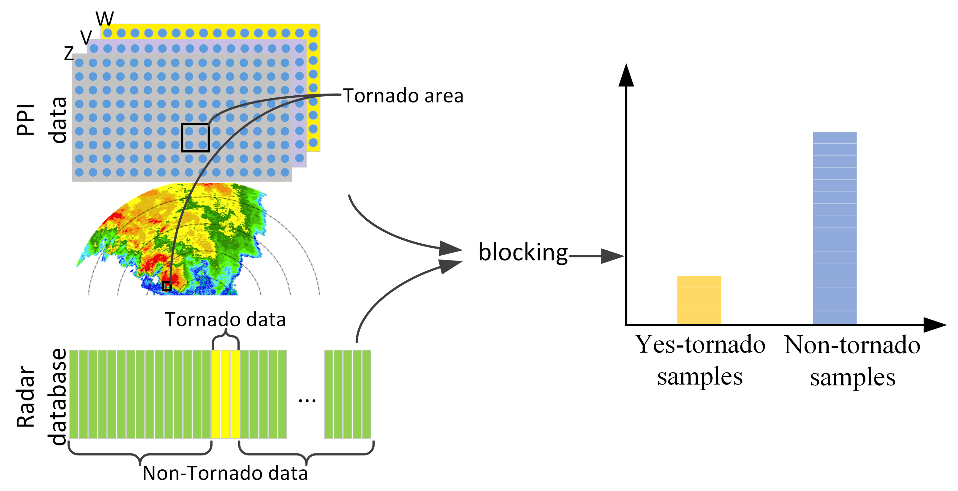
2.1. Weather Radar
2.2. Tornado Samples
3. Methods
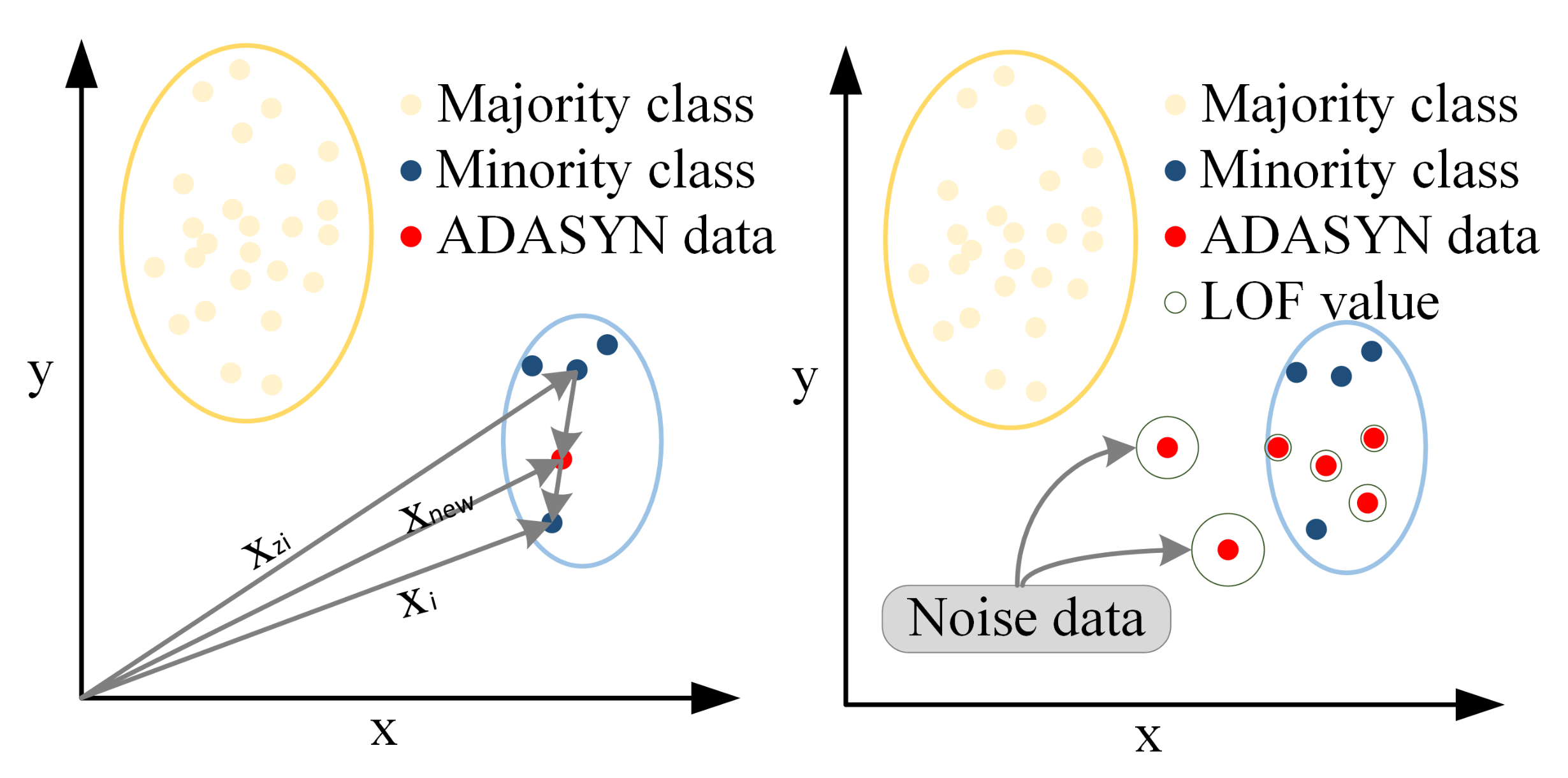
3.1. ADASYN
3.2. LOF
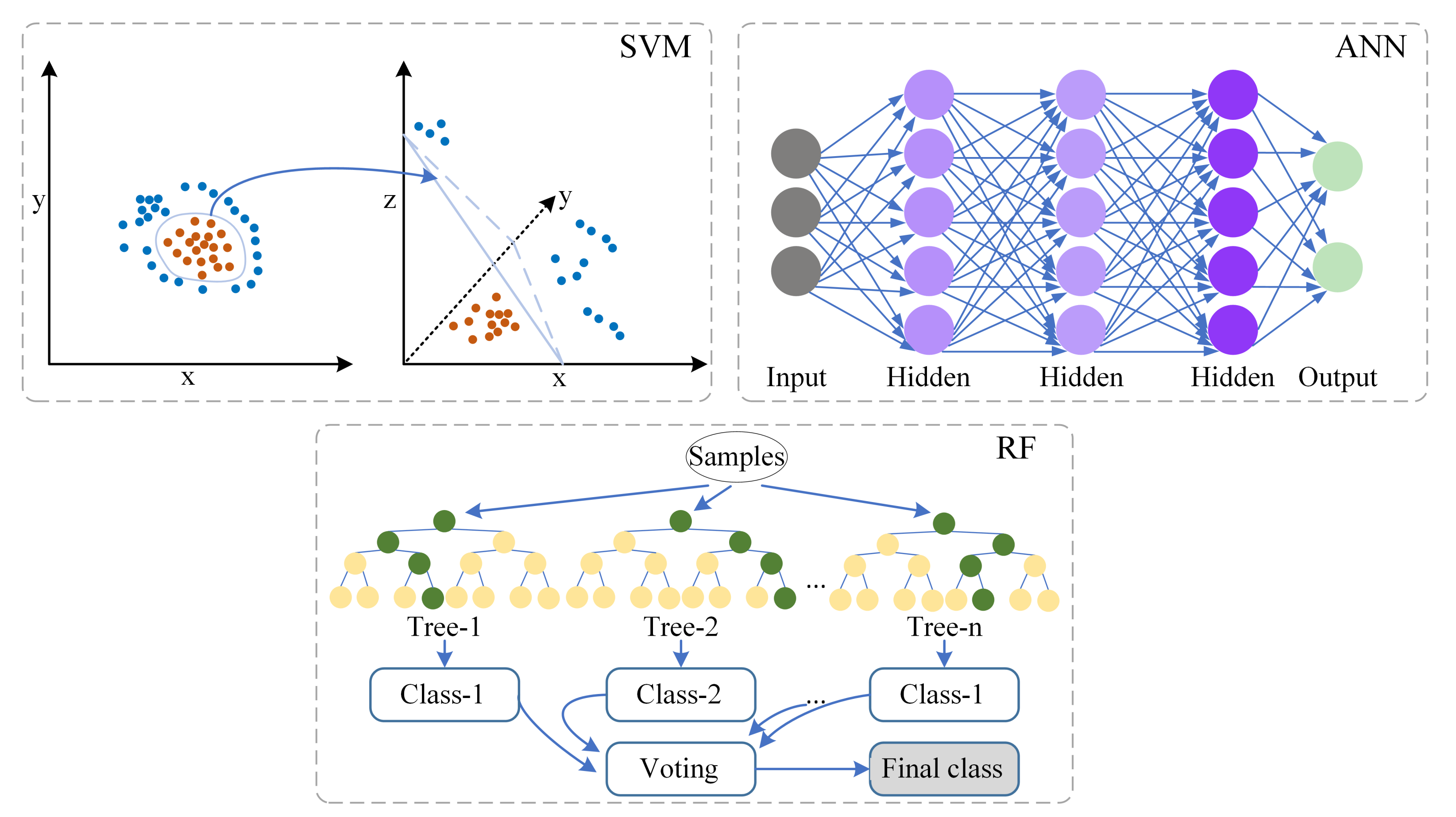
3.3. Machine Learning Models
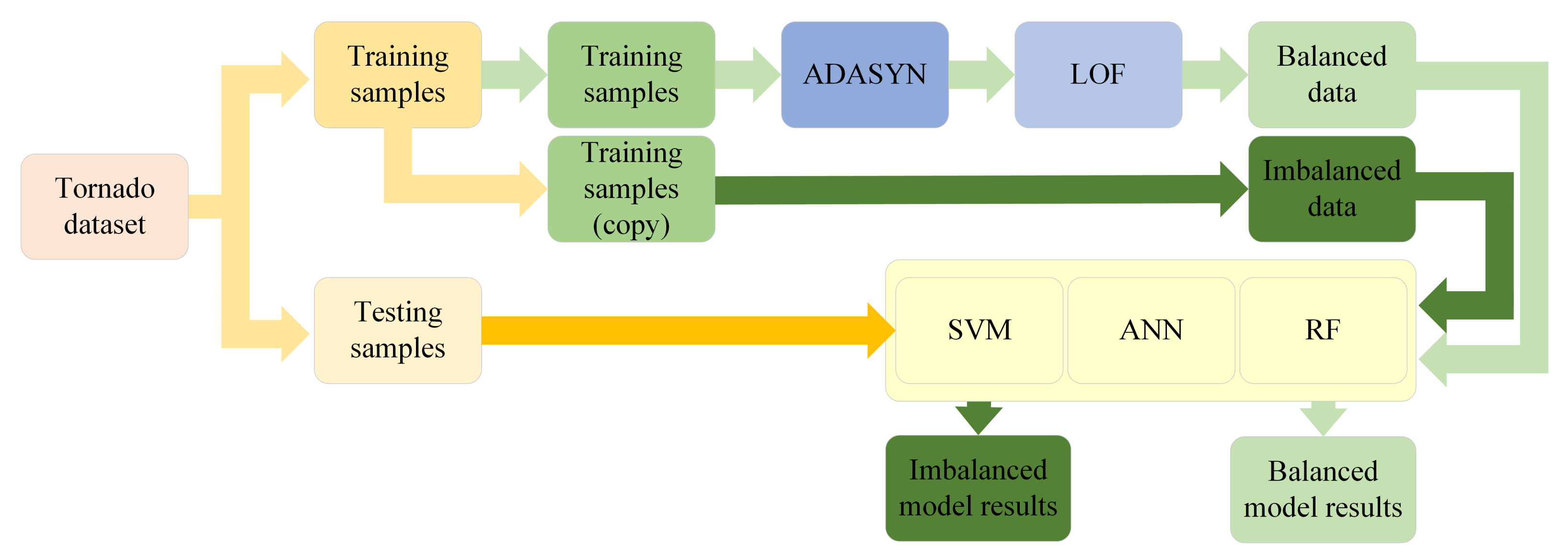
4. Experiments
4.1. Experiment 1
4.2. Experiment 2
5. Results and Discussion
5.1. Model Performance
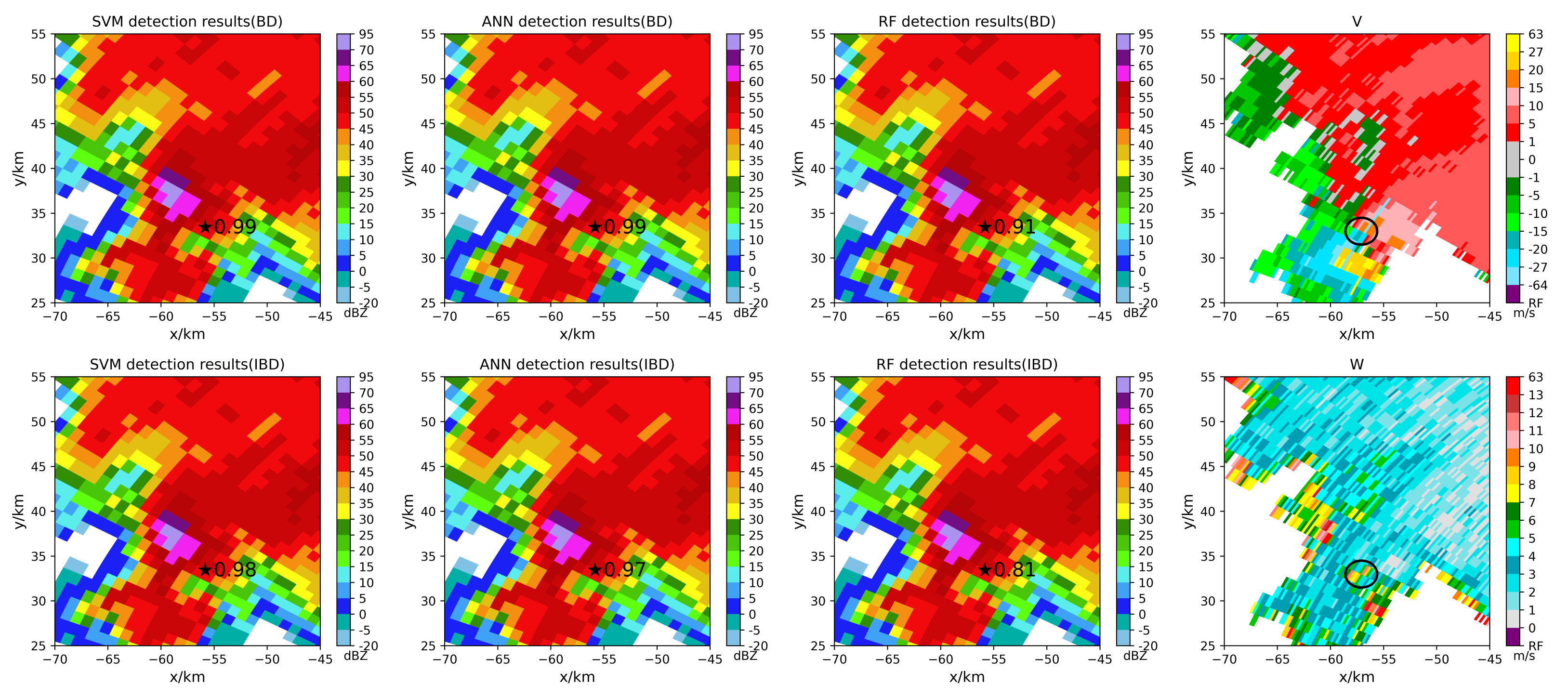
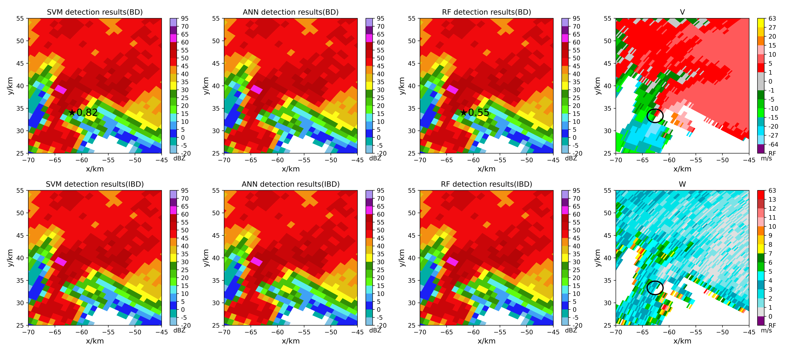
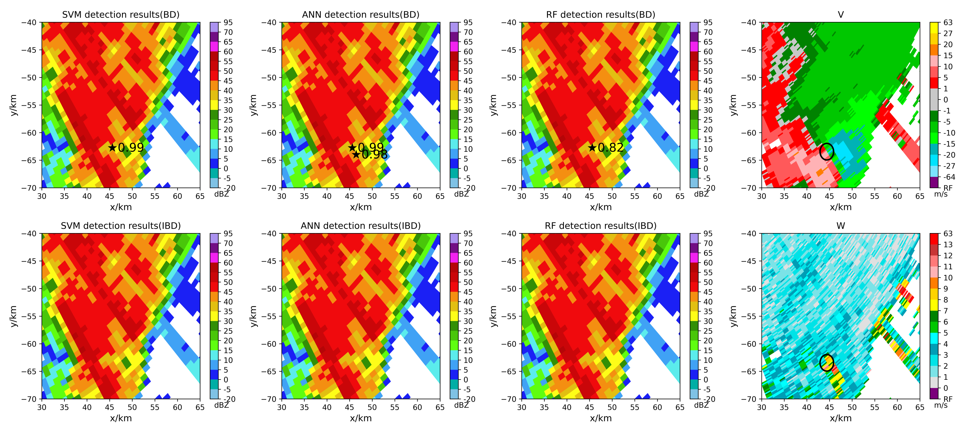
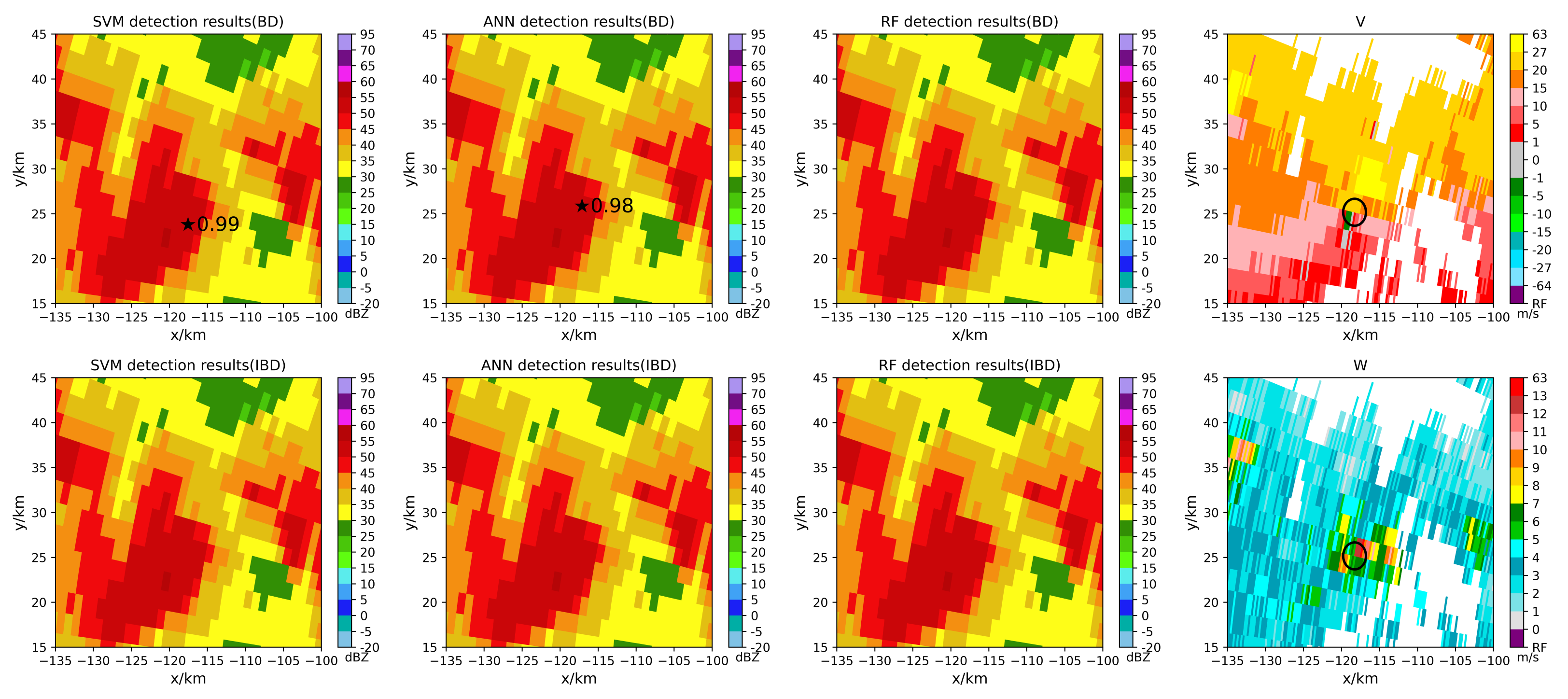
5.2. Tornado Detection Results
6. Conclusions
- After the ALA, the accuracy and precision are increased or decreased, the F1-score, G-mean, AUC, POD, CSI are significantly improved, the average performance is improved, and models have better noise immunity performance than the models without the approach.
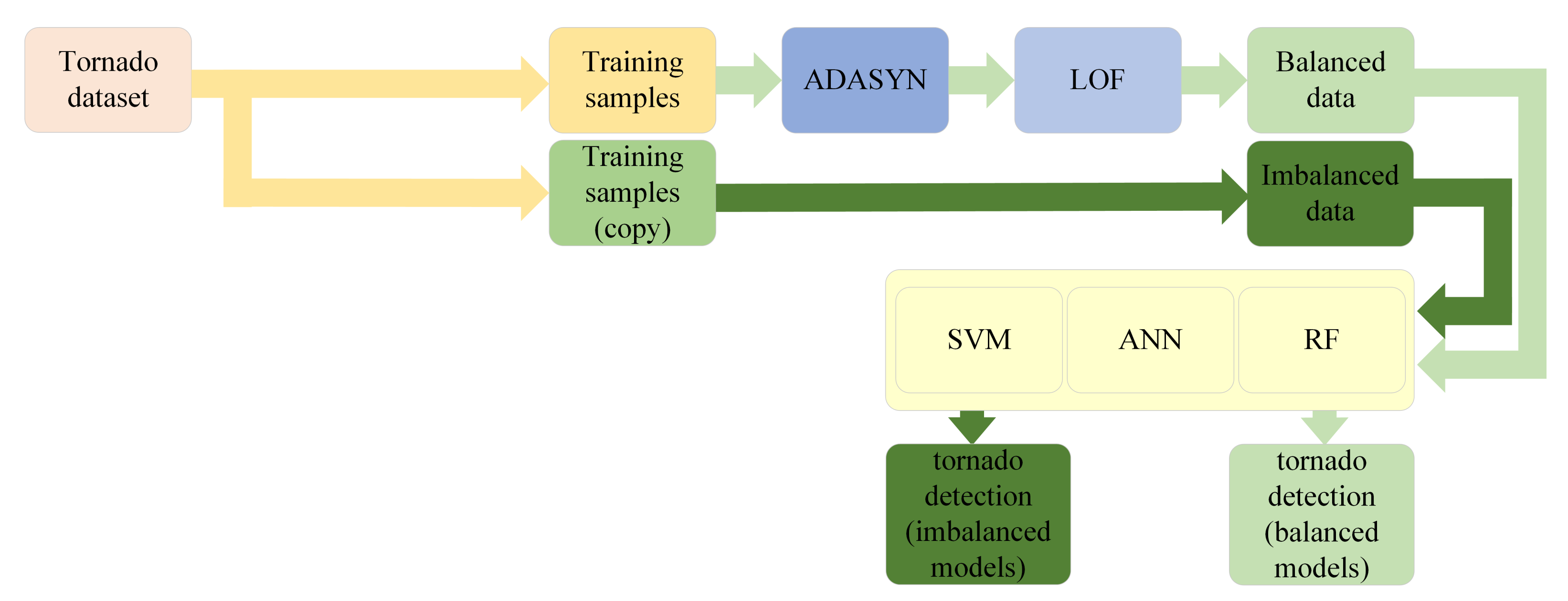
- Using specific tornado cases to test models, the balanced models have the following advantages after the ALA.
- In the early tornado warning, the models have the potential to increase the early warning time of tornadoes touching the ground.
- The balanced models can identify some tornadoes that cannot be identified by the imbalanced models.
- The models can identify tornadoes that cannot be detected due to the limitation of the tornado velocity signature (TVS) algorithm threshold.
- Compared with the ADASYN, SMOTE-LOF, and SMOTE algorithms, the ALA performs better in preprocessing imbalacned data if SVM or ANN is used as the classifier. If RF is used, the SMOTE-LOF algorithm could work better.
- optimize the k value of the ALA and appropriately reduce the dimension of sample features;
- study how to appropriately decrease the majority samples when applying the ALA;
- use more datasets (such as tornado datasets in the United States) to evaluate the ALA and apply outlier detection algorithms to detect tornadoes.
Author Contributions
Funding
Institutional Review Board Statement
Informed Consent Statement
Data Availability Statement
Acknowledgments
Conflicts of Interest
Abbreviations
| AI | Artificial Intelligence |
| ML | Machine Learning |
| ADASYN | Adaptive Synthetic |
| LOF | Local Outlier Factor |
| ALA | ADASYN-LOF algorithm |
| SVM | Supporting Vector Machine |
| ANN | Artificial Neural Network |
| RF | Random Forest |
| TVS | Tornado Velocity Signature |
| TDS | Tornado Debris Signature |
| CINRAD SA | the S-band China New Generation of Weather Radar |
| Z | Reflectivity |
| V | Doppler Velocity |
| W | Velocity Spectrum Width |
| VCP | Volume Coverage Pattern |
| PPI | Plan Position Indicator |
| BD | Balanced Dataset |
| IBD | Imbalanced Dataset |
Appendix A

| Feature | Description | Unit |
|---|---|---|
| r_average | the average value in the 4 × 4 Z block | dBZ |
| r_max | the maximum value in the 4 × 4 Z block | dBZ |
| r_min | the minimum value in the 4 × 4 Z block | dBZ |
| v_average | the average value in the 4 × 4 V block | m/s |
| v_max | the maximum value in the 4 × 4 V block | m/s |
| v_min | the minimum value in the 4 × 4 V block | m/s |
| w_average | the average value in the 4 × 4 W block | m/s |
| w_max | the maximum value in the 4 × 4 W block | m/s |
| w_min | the minimum value in the 4 × 4 W block | m/s |
| s_average | the average value of velocity shear in the 4 × 4 V block | 1/s |
| s_max | the maximum value of velocity shear in the 4 × 4 V block | 1/s |
| s_min | the minimum value of velocity shear in the 4 × 4 V block | 1/s |
| l_average | the average value of angular momentum in the 4 × 4 V block | m/s |
| l_max | the maximum value of angular momentum in the 4 × 4 V block | m/s |
| l_min | the minimum value of angular momentum in the 4 × 4 V block | m/s |
| vt_average | the average value of rotation speed in the 4 × 4 V block | m/s |
| vt_max | the maximum value of rotation speed in the 4 × 4 V block | m/s |
| vt_min | the minimum value of rotation speed in the 4 × 4 V block | m/s |
| c4_d_v_max | the maximum value of velocity difference in the 2 × 2 V block | m/s |
| c4_s_average | the average value of velocity shear in the 2 × 2 V block | 1/s |
| c4_s_max | the maximum value of velocity shear in the 2 × 2 V block | 1/s |
| c4_s_min | the minimum value of velocity shear in the 2 × 2 V block | 1/s |
| c4_l_average | the average value of angular momentum in the 2 × 2 V block | m/s |
| c4_l_max | the maximum value of angular momentum in the 2 × 2 V block | m/s |
| c4_l_min | the minimum value of angular momentum in the 2 × 2 V block | m/s |
| c4_vt_average | the average value of rotation speed in the 2 × 2 V block | m/s |
| c4_vt_max | the maximum value of rotation speed in the 2 × 2 V block | m/s |
| c4_vt_min | the minimum value of rotation speed in the 2 × 2 V block | m/s |
| w_range | the range value of velocity spectral width in the 4 × 4 W block | m/s |
| w_40 | the threshould greater than 40% velocity spectral width in the 4 × 4 W block | m/s |
| w_60 | the threshould greater than 60% velocity spectral width in the 4 × 4 W block | m/s |
| w_80 | the threshould greater than 80% velocity spectral width in the 4 × 4 W block | m/s |

| Evaluation | ADASYN-LOF | ADASYN | SMOTE-LOF | SMOTE | |
|---|---|---|---|---|---|
| ACC | 0.9277 | 0.9197 | 0.9237 | 0.9116 | |
| PRE | 0.7385 | 0.7164 | 0.7273 | 0.6957 | |
| F1-score | 0.8421 | 0.8276 | 0.8348 | 0.8136 | |
| SVM | G-mean | 0.9467 | 0.9416 | 0.9442 | 0.9363 |
| AUC | 0.9473 | 0.9423 | 0.9448 | 0.9373 | |
| POD | 0.9796 | 0.9796 | 0.9796 | 0.9796 | |
| FAR | 0.2615 | 0.2836 | 0.2727 | 0.3043 | |
| CSI | 0.7273 | 0.7059 | 0.7164 | 0.6857 | |
| ACC | 0.9438 | 0.9237 | 0.9398 | 0.9398 | |
| PRE | 0.9070 | 0.8947 | 0.9250 | 0.9048 | |
| F1-score | 0.8478 | 0.7816 | 0.8315 | 0.8352 | |
| ANN | G-mean | 0.8832 | 0.8246 | 0.8624 | 0.8718 |
| AUC | 0.8880 | 0.8369 | 0.8701 | 0.8778 | |
| POD | 0.7959 | 0.6939 | 0.7551 | 0.7755 | |
| FAR | 0.0930 | 0.1053 | 0.0750 | 0.0952 | |
| CSI | 0.7358 | 0.6415 | 0.7115 | 0.7170 | |
| ACC | 0.9438 | 0.9357 | 0.9478 | 0.9398 | |
| PRE | 0.9268 | 0.9231 | 0.9500 | 0.9722 | |
| F1-score | 0.8444 | 0.8182 | 0.8539 | 0.8235 | |
| RF | G-mean | 0.8740 | 0.8507 | 0.8762 | 0.8430 |
| AUC | 0.8803 | 0.8598 | 0.8828 | 0.8546 | |
| POD | 0.7755 | 0.7347 | 0.7755 | 0.7143 | |
| FAR | 0.0732 | 0.0769 | 0.0500 | 0.0278 | |
| CSI | 0.7308 | 0.6923 | 0.7451 | 0.7000 |
References
- Chen, J.; Cai, X.; Wang, H.; Kang, L.; Zhang, H.; Song, Y.; Zhu, H.; Zheng, W.; Li, F. Tornado climatology of China. Int. J. Climatol. 2018, 38, 2478–2489. [Google Scholar] [CrossRef]
- McCarthy, D.; Schaefer, J.; Edwards, R. What are we doing with (or to) the F-Scale. In Proceedings of the 23rd Conference on Severe Local Storms, St. Louis, MO, USA, 6–10 November 2006; Volume 5. [Google Scholar]
- Doswell, C.A., III; Brooks, H.E.; Dotzek, N. On the implementation of the enhanced Fujita scale in the USA. Atmos. Res. 2009, 93, 554–563. [Google Scholar] [CrossRef]
- Brown, R.A.; Lemon, L.R.; Burgess, D.W. Tornado detection by pulsed Doppler radar. Mon. Weather Rev. 1978, 106, 29–38. [Google Scholar] [CrossRef]
- Zrnić, D.; Burgess, D.; Hennington, L. Automatic detection of mesocyclonic shear with Doppler radar. J. Atmos. Ocean. Technol. 1985, 2, 425–438. [Google Scholar] [CrossRef][Green Version]
- Stumpf, G.J.; Witt, A.; Mitchell, E.D.; Spencer, P.L.; Johnson, J.; Eilts, M.D.; Thomas, K.W.; Burgess, D.W. The National Severe Storms Laboratory mesocyclone detection algorithm for the WSR-88D. Weather Forecast. 1998, 13, 304–326. [Google Scholar] [CrossRef]
- Mitchell, E.D.W.; Vasiloff, S.V.; Stumpf, G.J.; Witt, A.; Eilts, M.D.; Johnson, J.; Thomas, K.W. The national severe storms laboratory tornado detection algorithm. Weather Forecast. 1998, 13, 352–366. [Google Scholar] [CrossRef]
- Ryzhkov, A.V.; Schuur, T.J.; Burgess, D.W.; Zrnic, D.S. Polarimetric tornado detection. J. Appl. Meteorol. 2005, 44, 557–570. [Google Scholar] [CrossRef]
- Wang, Y.; Yu, T.Y.; Yeary, M.; Shapiro, A.; Nemati, S.; Foster, M.; Andra, D.L., Jr.; Jain, M. Tornado detection using a neuro–fuzzy system to integrate shear and spectral signatures. J. Atmos. Ocean. Technol. 2008, 25, 1136–1148. [Google Scholar] [CrossRef]
- Alberts, T.A.; Chilson, P.B.; Cheong, B.; Palmer, R. Evaluation of weather radar with pulse compression: Performance of a fuzzy logic tornado detection algorithm. J. Atmos. Ocean. Technol. 2011, 28, 390–400. [Google Scholar] [CrossRef]
- Wang, Y.; Yu, T.Y. Novel tornado detection using an adaptive neuro-fuzzy system with S-band polarimetric weather radar. J. Atmos. Ocean. Technol. 2015, 32, 195–208. [Google Scholar] [CrossRef]
- Hill, A.J.; Herman, G.R.; Schumacher, R.S. Forecasting Severe Weather with Random Forests. Mon. Weather Rev. 2020, 148, 2135–2161. [Google Scholar] [CrossRef]
- Basalyga, J.N.; Barajas, C.A.; Gobbert, M.K.; Wang, J.W. Performance Benchmarking of Parallel Hyperparameter Tuning for Deep Learning Based Tornado Predictions. Big Data Res. 2021, 25, 100212. [Google Scholar] [CrossRef]
- Rout, N.; Mishra, D.; Mallick, M.K. Handling imbalanced data: A survey. In International Proceedings on Advances in Soft Computing, Intelligent Systems and Applications; Springer: Berlin/Heidelberg, Germany, 2018; pp. 431–443. [Google Scholar]
- Kaur, H.; Pannu, H.S.; Malhi, A.K.J.A.C.S. A systematic review on imbalanced data challenges in machine learning: Applications and solutions. ACM Comput. Surv. 2019, 52, 1–36. [Google Scholar] [CrossRef]
- Lin, W.C.; Tsai, C.F.; Hu, Y.H.; Jhang, J.S. Clustering-based undersampling in class-imbalanced data. Inf. Sci. 2017, 409, 17–26. [Google Scholar] [CrossRef]
- Choi, W.; Heo, J.; Ahn, C. Development of Road Surface Detection Algorithm Using CycleGAN-Augmented Dataset. Sensors 2021, 21, 7769. [Google Scholar] [CrossRef] [PubMed]
- Setiawan, B.D.; Serdült, U.; Kryssanov, V. A Machine Learning Framework for Balancing Training Sets of Sensor Sequential Data Streams. Sensors 2021, 21, 6892. [Google Scholar] [CrossRef]
- Trafalis, T.B.; Adrianto, I.; Richman, M.B.; Lakshmivarahan, S. Machine-learning classifiers for imbalanced tornado data. Comput. Manag. Sci. 2014, 11, 403–418. [Google Scholar] [CrossRef]
- Maalouf, M.; Trafalis, T.B. Robust weighted kernel logistic regression in imbalanced and rare events data. Comput. Stat. Data Anal. 2011, 55, 168–183. [Google Scholar] [CrossRef]
- Maalouf, M.; Siddiqi, M. Weighted logistic regression for large-scale imbalanced and rare events data. Knowl.-Based Syst. 2014, 59, 142–148. [Google Scholar] [CrossRef]
- Maalouf, M.; Homouz, D.; Trafalis, T.B. Logistic regression in large rare events and imbalanced data: A performance comparison of prior correction and weighting methods. Comput. Intell. 2018, 34, 161–174. [Google Scholar] [CrossRef]
- He, H.B.; Garcia, E.A. Learning from Imbalanced Data. IEEE Trans. Knowl. Data Eng. 2009, 21, 1263–1284. [Google Scholar] [CrossRef]
- Haixiang, G.; Yijing, L.; Shang, J.; Mingyun, G.; Yuanyue, H.; Bing, G. Learning from class-imbalanced data: Review of methods and applications. Expert Syst. Appl. 2017, 73, 220–239. [Google Scholar] [CrossRef]
- Yu, L.; Zhou, N. Survey of Imbalanced Data Methodologies. arXiv 2021, arXiv:2104.02240. [Google Scholar]
- Chawla, N.V.; Bowyer, K.W.; Hall, L.O.; Kegelmeyer, W.P. SMOTE: Synthetic minority over-sampling technique. J. Artif. Intell. Res. 2002, 16, 321–357. [Google Scholar] [CrossRef]
- He, H.; Bai, Y.; Garcia, E.A.; Li, S. ADASYN: Adaptive synthetic sampling approach for imbalanced learning. In Proceedings of the 2008 IEEE International Joint Conference on Neural Networks (IEEE World Congress on Computational Intelligence), Hong Kong, China, 1–8 June 2008; pp. 1322–1328. [Google Scholar]
- Susan, S.; Kumar, A. SSOMaj-SMOTE-SSOMin: Three-step intelligent pruning of majority and minority samples for learning from imbalanced datasets. Appl. Soft Comput. 2019, 78, 141–149. [Google Scholar] [CrossRef]
- Ye, X.C.; Li, H.M.; Imakura, A.; Sakurai, T. An oversampling framework for imbalanced classification based on Laplacian eigenmaps. Neurocomputing 2020, 399, 107–116. [Google Scholar] [CrossRef]
- Tripathi, A.; Chakraborty, R.; Kopparapu, S.K. A novel adaptive minority oversampling technique for improved classification in data imbalanced scenarios. In Proceedings of the 2020 25th International Conference on Pattern Recognition (ICPR), Milan, Italy, 10–15 January 2021; pp. 10650–10657. [Google Scholar]
- Maulidevi, N.U.; Surendro, K. SMOTE-LOF for noise identification in imbalanced data classification. J. King Saud-Univ.-Comput. Inf. Sci. 2021. [Google Scholar] [CrossRef]
- Heinselman, P.; LaDue, D.; Kingfield, D.M.; Hoffman, R. Tornado warning decisions using phased-array radar data. Weather Forecast. 2015, 30, 57–78. [Google Scholar] [CrossRef]
- Jun, L.; Honggen, Z.; Jianbing, L.; Xinan, L. Research on the networking strategy of tornado observation network in Northern Jiangsu based on X-band weather radar. In Proceedings of the 2019 International Conference on Meteorology Observations (ICMO), Chengdu, China, 28–31 December 2019; pp. 1–4. [Google Scholar]
- Adachi, T.; Mashiko, W. High temporal-spatial resolution observation of tornadogenesis in a shallow supercell associated with Typhoon Hagibis (2019) using phased array weather radar. Geophys. Res. Lett. 2020, 47, e2020GL089635. [Google Scholar] [CrossRef]
- Yoshida, S.; Misumi, R.; Maesaka, T. Early Detection of Convective Echoes and Their Development Using a Ka-Band Radar Network. Weather Forecast. 2021, 36, 253–264. [Google Scholar] [CrossRef]
- Zhang, X.; He, J.; Zeng, Q.; Shi, Z. Weather Radar Echo Super-Resolution Reconstruction Based on Nonlocal Self-Similarity Sparse Representation. Atmosphere 2019, 10, 254. [Google Scholar] [CrossRef]
- Chen, H.; Chandrasekar, V. Real-time wind velocity retrieval in the precipitation system using high-resolution operational multi-radar network. In Remote Sensing of Aerosols, Clouds, and Precipitation; Elsevier: Amsterdam, The Netherlands, 2018; pp. 315–339. [Google Scholar]
- Breunig, M.M.; Kriegel, H.P.; Ng, R.T.; Sander, J. LOF: Identifying density-based local outliers. In Proceedings of the 2000 ACM SIGMOD International Conference on Management of Data, Dallas, TX, USA, 16–18 May 2000; pp. 93–104. [Google Scholar]
- Cortes, C.; Vapnik, V. Support-vector networks. Mach. Learn. 1995, 20, 273–297. [Google Scholar] [CrossRef]
- Chang, C.C.; Lin, C.J. LIBSVM: A Library for Support Vector Machines. Acm Trans. Intell. Syst. Technol. 2011, 2, 1–27. [Google Scholar] [CrossRef]
- Platt, J. Probabilistic outputs for support vector machines and comparisons to regularized likelihood methods. Adv. Large Margin Classif. 1999, 10, 61–74. [Google Scholar]
- Chen, H.; Zhang, X.; Liu, Y.; Zeng, Q. Generative adversarial networks capabilities for super-resolution reconstruction of weather radar echo images. Atmosphere 2019, 10, 555. [Google Scholar] [CrossRef]
- Geiss, A.; Hardin, J.C. Radar super resolution using a deep convolutional neural network. J. Atmos. Ocean. Technol. 2020, 37, 2197–2207. [Google Scholar] [CrossRef]
- Maind, S.B.; Wankar, P. Research paper on basic of artificial neural network. Int. J. Recent Innov. Trends Comput. Commun. 2014, 2, 96–100. [Google Scholar]
- Agatonovic-Kustrin, S.; Beresford, R. Basic concepts of artificial neural network (ANN) modeling and its application in pharmaceutical research. J. Pharm. Biomed. Anal. 2000, 22, 717–727. [Google Scholar] [CrossRef]
- Zhang, Z. Artificial neural network. In Multivariate Time Series Analysis in Climate and Environmental Research; Springer: Berlin/Heidelberg, Germany, 2018; pp. 1–35. [Google Scholar]
- Breiman, L. Bagging predictors. Mach. Learn. 1996, 24, 123–140. [Google Scholar] [CrossRef]
- Breiman, L. Random forests. Mach. Learn. 2001, 45, 5–32. [Google Scholar] [CrossRef]
- Genuer, R.; Poggi, J.M.; Tuleau-Malot, C. Variable selection using random forests. Pattern Recognit. Lett. 2010, 31, 2225–2236. [Google Scholar] [CrossRef]
- Breiman, L.; Friedman, J.H.; Olshen, R.A.; Stone, C.J. Classification and Regression Trees; Routledge: London, UK, 2017. [Google Scholar]
- Elaidi, H.; Benabbou, Z.; Abbar, H. A comparative study of algorithms constructing decision trees: Id3 and c4.5. In Proceedings of the International Conference on Learning and Optimization Algorithms: Theory and Applications, Rabat, Morocco, 2–5 May 2018; pp. 1–5. [Google Scholar]
- Peerbhay, K.Y.; Mutanga, O.; Ismail, R. Random Forests Unsupervised Classification: The Detection and Mapping of Solanum mauritianum Infestations in Plantation Forestry Using Hyperspectral Data. IEEE J. Sel. Top. Appl. Earth Obs. Remote Sens. 2015, 8, 3107–3122. [Google Scholar] [CrossRef]
- Dong, Y.N.; Du, B.; Zhang, L.P. Target Detection Based on Random Forest Metric Learning. IEEE J. Sel. Top. Appl. Earth Obs. Remote Sens. 2015, 8, 1830–1838. [Google Scholar] [CrossRef]
- Dong, L.; Du, H.; Mao, F.; Han, N.; Li, X.; Zhou, G.; Zheng, J.; Zhang, M.; Xing, L.; Liu, T. Very high resolution remote sensing imagery classification using a fusion of random forest and deep learning technique—Subtropical area for example. IEEE J. Sel. Top. Appl. Earth Obs. Sens. 2019, 13, 113–128. [Google Scholar] [CrossRef]
- Wang, Z.Y.; Zuo, R.G.; Dong, Y.N. Mapping of Himalaya Leucogranites Based on ASTER and Sentinel-2A Datasets Using a Hybrid Method of Metric Learning and Random Forest. IEEE J. Sel. Top. Appl. Earth Obs. Remote Sens. 2020, 13, 1925–1936. [Google Scholar] [CrossRef]
- McGovern, A.; John Gagne, D.; Troutman, N.; Brown, R.A.; Basara, J.; Williams, J.K. Using spatiotemporal relational random forests to improve our understanding of severe weather processes. Stat. Anal. Data Mining ASA Data Sci. J. 2011, 4, 407–429. [Google Scholar] [CrossRef]
- Herman, G.R.; Schumacher, R.S. Money Doesn’t Grow on Trees, but Forecasts Do: Forecasting Extreme Precipitation with Random Forests. Mon. Weather Rev. 2018, 146, 1571–1600. [Google Scholar] [CrossRef]


| True Class | |||
|---|---|---|---|
| Positive (yes-tornado) | Negative (non-tornado) | ||
| Y (yes-tornado) | TP (True Positives) | FP (False Positives) | |
| Model prediction | N (non-tornado) | FN (False Negatives) | TN (True Negatives) |
| Column counts | |||
| Warning | |||
|---|---|---|---|
| YES | NO | ||
| YES | X | Y | |
| weather event | NO | Z | W |
| Model | Evaluation | ADASYN-LOF | NONE |
|---|---|---|---|
| ACC | 0.9277 | 0.9317 | |
| PRE | 0.7385 | 0.9211 | |
| F1-score | 0.8421 | 0.8046 | |
| SVM | G-mean | 0.9467 | 0.8388 |
| AUC | 0.9473 | 0.8496 | |
| POD | 0.9796 | 0.7143 | |
| FAR | 0.2615 | 0.0790 | |
| CSI | 0.7273 | 0.6731 | |
| ACC | 0.9438 | 0.9237 | |
| PRE | 0.9070 | 0.8750 | |
| F1-score | 0.8478 | 0.7856 | |
| ANN | G-mean | 0.8832 | 0.8354 |
| AUC | 0.8880 | 0.8446 | |
| POD | 0.7959 | 0.7142 | |
| FAR | 0.0930 | 0.1250 | |
| CSI | 0.7358 | 0.6481 | |
| ACC | 0.9438 | 0.8916 | |
| PRE | 0.9268 | 0.9583 | |
| F1-score | 0.8444 | 0.6301 | |
| RF | G-mean | 0.8740 | 0.6834 |
| AUC | 0.8803 | 0.7322 | |
| POD | 0.7755 | 0.4694 | |
| FAR | 0.0732 | 0.0417 | |
| CSI | 0.7308 | 0.4600 |
Publisher’s Note: MDPI stays neutral with regard to jurisdictional claims in published maps and institutional affiliations. |
© 2022 by the authors. Licensee MDPI, Basel, Switzerland. This article is an open access article distributed under the terms and conditions of the Creative Commons Attribution (CC BY) license (https://creativecommons.org/licenses/by/4.0/).
Share and Cite
Qing, Z.; Zeng, Q.; Wang, H.; Liu, Y.; Xiong, T.; Zhang, S. ADASYN-LOF Algorithm for Imbalanced Tornado Samples. Atmosphere 2022, 13, 544. https://doi.org/10.3390/atmos13040544
Qing Z, Zeng Q, Wang H, Liu Y, Xiong T, Zhang S. ADASYN-LOF Algorithm for Imbalanced Tornado Samples. Atmosphere. 2022; 13(4):544. https://doi.org/10.3390/atmos13040544
Chicago/Turabian StyleQing, Zhipeng, Qiangyu Zeng, Hao Wang, Yin Liu, Taisong Xiong, and Shihao Zhang. 2022. "ADASYN-LOF Algorithm for Imbalanced Tornado Samples" Atmosphere 13, no. 4: 544. https://doi.org/10.3390/atmos13040544
APA StyleQing, Z., Zeng, Q., Wang, H., Liu, Y., Xiong, T., & Zhang, S. (2022). ADASYN-LOF Algorithm for Imbalanced Tornado Samples. Atmosphere, 13(4), 544. https://doi.org/10.3390/atmos13040544