Article

Low-Latitude Ionospheric Responses and Coupling to the February 2014 Multiphase Geomagnetic Storm from GNSS, Magnetometers, and Space Weather Data

1
School of Remote Sensing and Geomantic Engineering, Nanjing University of Information Science and Technology, Nanjing 210044, China
2
Department of Physics and Mathematics, University of Alcalá, 28801 Alcalá de Henares, Madrid, Spain
3
Department of Physics and Astronomy, University of Nigeria, Nsukka 400221, Nigeria
4
GNSS and Space Weather Lab, Department of Space Science, National Center of GIS and Space Application, Institute of Space Technology, Islamabad 44000, Pakistan
5
Sorbonne Université, Ecole Polytechnique, Institut Polytechnique de Paris, Université Paris Saclay, Observatoire de Paris, CNRS, Laboratoire de Physique des Plasmas (LPP), 75005 Paris, France
6
Institute of Solar-Terrestrial Physics of Siberian Branch of Russian Academy of Sciences, 664033 Irkutsk, Russia
7
Physics Department & Geophysical Institute, University of Alaska Fairbanks, Fairbanks, AK 99775-7320, USA
8
Department of Physics, Federal University of Technology, Akure 340252, Nigeria
9
Shanghai Astronomical Observatory, Chinese Academy of Sciences, Shanghai 200030, China
10
School of Surveying and Land Information Engineering, Henan Polytechnic University, Jiaozuo 454003, China
*
Author to whom correspondence should be addressed.
Atmosphere 2022, 13(4), 518; https://doi.org/10.3390/atmos13040518
Submission received: 16 February 2022 / Revised: 19 March 2022 / Accepted: 20 March 2022 / Published: 24 March 2022

Abstract

:
The ionospheric response and the associated mechanisms to geomagnetic storms are very complex, particularly during the February 2014 multiphase geomagnetic storm. In this paper, the low-latitude ionosphere responses and their coupling mechanisms, during the February 2014 multiphase geomagnetic storm, are investigated from ground-based magnetometers and global navigation satellite system (GNSS), and space weather data. The residual disturbances between the total electron content (TEC) of the International GNSS Service (IGS) global ionospheric maps (GIMs) and empirical models are used to investigate the storm-time ionospheric responses. Three clear sudden storm commencements (SSCs) on 15, 20, and 23 February are detected, and one high speed solar wind (HSSW) event on 19 February is found with the absence of classical SSC features due to a prevalent magnetospheric convection. The IRI-2012 shows insufficient performance, with no distinction between the events and overestimating approximately 20 TEC units (TECU) with respect to the actual quiet-time TEC. Furthermore, the median average of the IGS GIMs TEC during February 2014 shows enhanced values in the southern hemisphere, whereas the IRI-2012 lacks this asymmetry. Three low-latitude profiles extracted from the IGS GIM data revealed up to 20 TECU enhancements in the differential TEC. From these profiles, longer-lasting TEC enhancements are observed at the dip equator profiles than in the profiles of the equatorial ionospheric anomaly (EIA) crests. Moreover, a gradual increase in the global electron content (GEC) shows approximately 1 GEC unit of differential intensification starting from the HSSW event, while the IGS GIM profiles lack this increasing gradient, probably located at higher latitudes. The prompt penetration electric field (PPEF) and equatorial electrojet (EEJ) indices estimated from magnetometer data show strong variability after all four events, except the EEJ’s Asian sector. The low-latitude ionosphere coupling is mainly driven by the variable PPEF, DDEF (disturbance dynamo electric fields), and Joule heating. The auroral electrojet causing eastward PPEF may control the EIA expansion in the Asian sector through the dynamo mechanism, which is also reflected in the solar-quiet current intensity variability.

1. Introduction

Short-term ionospheric irregularities, especially those triggered by geomagnetic storms, can be monitored by numerous techniques and instruments, including global navigation satellite systems (GNSS) receivers, ground-based magnetometers, ionosondes, satellite instruments, etc. One of the most accurate and massive-data delivery methods uses the dual-frequency GNSS observations, which have been widely used to estimate regional and global total electron content (TEC) variability [1,2,3,4,5]. Ionospheric fluctuations and irregularities are mainly caused by the solar cycle and geomagnetic activity, which drive complex processes in the upper atmosphere. The meteorological activity also largely influences ionosphere disturbances [6]. The accurate understanding and modeling of these variations are extremely important for applications and for society, for example, for GNSS positioning, satellite communication infrastructures, and Earth observation through remote sensing techniques.
There is a great deal of different models, but they still have much to be desired in the way of accuracy, especially during complex geomagnetic storms. A list of well-known models includes, e.g., the Klobuchar model [7], the SAMI model [8], the NTCM model [9], the NeQuick model [10,11], or the International Reference Ionosphere (IRI) model [12]. However, the complex processes in the upper atmosphere during geomagnetic storms cause difficulties for accurate modeling; the existing models can only deliver monthly averages of the actual variability, especially during magnetically quiet times.
During the last few decades, the understanding of ionosphere responses during geomagnetic storms has remained a complex task in the fields of solar–terrestrial interactions and magnetosphere–ionosphere–thermosphere coupling [13,14,15,16]. Ionospheric behavior during geomagnetic storms is being regulated by several electrodynamic and chemical processes, and its accurate modeling for practical applications is still a major challenge. These processes are largely affected by the variable solar plasma wind via magnetospheric energy input during geomagnetic storms and are further electromagnetically coupled to the ionosphere. Major geomagnetic storms usually occur after extreme solar events, especially Earth-directed coronal mass ejections (CMEs) and co-rotating interaction regions (CIRs). CMEs can produce stronger storms than CIRs and are usually initiated by a southward interplanetary magnetic field (IMF), which enhances the night-side convection and increases the ring current. When CIRs and CMEs reach Earth, solar wind/magnetosphere coupling processes generate a rapid increase in Poynting flux; they result in an enhancement of Joule heating, which leads to disturbances in upper atmosphere composition, temperature, density, and winds (e.g., [4,17,18,19,20]).
The ionosphere itself is mainly created by processes of energy-absorption, ionization, and dissociation of molecules due to variable incoming extreme ultraviolet (EUV) and X radiation from the Sun, as well as high-latitude thermospheric Joule heating and precipitation of energetic particles due to solar wind and magnetospheric forcing, especially during geomagnetic storms. At the geomagnetic equator, the magnetic field is horizontal, and three factors mainly govern the equatorial ionosphere during magnetic quiet periods:
  • The Equatorial Ionization Anomaly (EIA) [21,22], where the E × B drift moves plasma vertically as a result of the east/west electric field. At high altitudes, the pressure gradients and gravity become important and cause plasma to diffuse along the lines of Earth’s magnetic field. As a result, two peaks of electron density at ±15° from the geomagnetic equator and a trough of electron density at the geomagnetic equator are created.
  • Equatorial Electrojet (EEJ) [23] along the magnetic equator as a result of an ionospheric electric current at altitudes of about 110 km. This current is approximately twice as strong as the mid-latitude solar-quiet (Sq) ionospheric current [24].
  • Equatorial plasma bubbles (EPB) related to the pre-reversal enhancement (PRE) of the eastward electric field around sunset [25,26,27]. The electric field is eastward during the day and westward during night, and the PRE occurs as an eastward electric field increases before turning westward at sunset. The PRE associated with the sharp ionospheric depletion at sunset creates a Rayleigh Taylor instability at the origin of EPB.
During geomagnetic storms, the equatorial ionosphere is coupled with the high latitude ionosphere through electrodynamics and related factors:
  • Transmission of electric fields related to the motion of particles in the magnetosphere, namely Prompt Penetration Electric Field (PPEF) [28].
  • The electrojet in the auroral zone (ionospheric electric currents) dissipates energy through Joule heating and produces a thermal expansion of the atmosphere (variations in pressure, temperature, and motion) [29].
  • Motions of the neutral atmosphere by disturbance dynamo electric fields (DDEF) [30,31].
TEC enhancements during geomagnetic storms have been widely studied on regional and global scales. Several authors have specifically looked for latitudinal and longitudinal dependencies with multi-instrumental observations (e.g., [32,33,34,35]). Ref. [30] studied the modelling of DDEF at mid-latitudes and showed the existence of electric current cells, which is a very interesting finding for studies on low-latitude magnetic disturbances due to ionospheric DDEF on a planetary scale. Ref. [36] observed similar effects at two zonal sectors separated by 12 h in LST during an intense geomagnetic storm. The southward IMF Bz caused an eastward electric-field drift in the daytime sector, and then westward in the night side [37]. Ref. [38] showed the redistribution of plasma in the low-latitude ionosphere under electrodynamics processes of the E and F regions, and [39] examined the low-latitude ionosphere for different longitudes. They showed no significant longitudinal variations in the electron densities.
The EIA crests can reach up to ±20 degrees of the magnetic latitude during geomagnetic storms [40], and the PPEF of westward polarity during the night side has Earth directed to a downward drift, which results in plasma depletion at the low-latitude regions. Ref. [41] performed a complete analysis of the storm-time ionospheric responses at different stations in the equatorial regions and provided similar evidence during storm time periods in the form of ion drift and EEJ variability, but the authors found a lack of variations in the ionosphere due to PPEF, except for South America. The authors investigated the correlation of storm-time enhancements in South America during the local morning with PPEF peaks, while the African and Asian sectors showed ionospheric variations before the PPEF. Ionospheric variations before the PPEF have been shown in the African and Asian sectors [41], where the energetic particle input may strengthen the enhancements of TEC. Ref. [42] investigated TEC enhancements at the low-latitude GNSS stations of Japan using a 27-day running-median window and stated a possible relation to the equatorial crest expansion. The expansion of the EIA to mid-latitude regions has been reported in [16]. The authors investigated the main phase of the August 2018 geomagnetic storm in the South American sector using GNSS TEC and other satellite data. In their work, storm-time ionospheric variations were attributed to PPEF and DDEF variability, which prompted EIA expansion to higher latitude regions. Ref. [40] studied the same storm and found medium-scale positive and negative ionospheric disturbances at middle and high latitudes that were attributed to a storm-enhanced density (SED)-plume, mid-latitude ionospheric trough, particle precipitation in the auroral zone, and equatorial plasma bubbles in South America.
This paper studies the low-latitude ionospheric variations and coupling mechanisms during the multiphase geomagnetic storm in February 2014. Ref. [43] studied the multiple signatures of this particular storm using data from Japan and Egypt geomagnetic stations and from the Van Allen Prove satellites (Applied Physics Laboratory, Laurel, MS, USA). It was shown that Pi2 pulsations (period range from 40 to 150 s) may have originated from the ionospheric current systems rather than the cavity resonance mode. Their work shows the magnetospheric variability during this complex multiphase storm but without further study on the coupled ionospheric variability. A clear understanding of the TEC variations during these kinds of events is very important for ionospheric modeling and applications, and very few studies on ionospheric variability during this multiphase storm, or similar events, can be found in the literature. In this paper, we present a study of the ionosphere responses to this complex storm using multiple GNSS, ground magnetometers, and solar wind data. There is further identification of possible discrepancies when compared to a typical isolated storm. In Section 2, there is a brief introduction to the materials and methods used in this study. Then, in Section 3, the results are presented with detailed descriptions and highlights. In Section 4, some explanations and discussions are given, and, finally, a summary of conclusions is provided in Section 5.

2. Data and Methods

2.1. Solar Wind and Geomagnetic Indices

In order to detect the solar contribution and coupling to ionospheric variability, solar wind and geomagnetic indices from the OMNIweb database (https://omniweb.gsfc.nasa.gov/, accessed date: 20 January 2021) [44] are used along with data from the International Service of Geomagnetic Indices (ISGI) website, which is available at http://isgi.unistra.fr/data_download.php (accessed date: 29 January 2021). There is the use of the solar wind (SW) plasma speed, temperature, pressure, proton density, beta parameter, and density ratio between alpha and proton particle, and also the IMF Bz component and total Bt IMF, the eastward zonal electric fields (Ey), the geomagnetic auroral indices AE and Am indices, and the equatorial SYM-H and Dst indices. Here, the symmetric disturbance field in H, SYM-H, is essentially the same as Sugiura’s hourly Dst index. The main difference is the time resolution, where the effects of the solar wind dynamic pressure variations during geomagnetic storms may be more clearly seen in the SYM-H than in the hourly Dst index. As compared to the SYM-H and Dst indices that measure the intensity of the globally symmetrical EEJ (the “ring current”), the Am index is susceptible to any geophysical current system, including magnetopause currents, field-aligned currents, or auroral electrojet. The ASY-D and ASY-H indices represent the range between the maximum and the minimum deviations of the magnetic D and H components, and usually are more suitable to monitor disturbances globally and in the polar regions, similar to the Am index (for a description of various geomagnetic indices, see [45]). Note also Ey = −Vx × Bz moves the plasma in the magnetosphere from the tail to Earth and creates the ring current.
Ref. [46] demonstrated that the merging electric field (Em) is a physical quantity that closely correlates with upper atmosphere variations during geomagnetic storms. The Em assumes that there is an equal magnitude of the electric field in the solar wind, the magnetosheath, and on the magnetospheric sides of the magnetopause [47]. We calculate this variable as follows:
E m = v S W B y 2 + B z 2 sin 2 ( θ 2 )
In this equation, By and Bz are the IMF components, vSW is the solar wind speed, and θ is the IMF clock angle in Geocentric Solar Magnetospheric (GSM) coordinates.

2.2. Vertical TEC from GNSS Stations in Africa

Slant TEC (sTEC) from ground-based GNSS Africa Geodetic Reference Network (AFREF, http://afrefdata.org, accessed on 29 January 2021) is used to study the low-latitude ionospheric variations in the African sector during the multiphase storms of February, 2014. AFREF stores input GNSS data for sTEC calculation in Receiver Independent Exchange Format (RINEX) [48] with 30 s cadences. To characterize the response to the storm, sTEC is converted into vTEC using GPS-TEC analysis software tools [1]. Table 1 shows the coordinates of the GNSS stations.
The median-average of February is used as a background vTEC for the analyses of disturbances to obtain the relative deviation of the daily values. The TEC deviation from the TEC background is referred to as relative TEC change (rTEC). Here, the threshold was set at |rTEC| ≥ 30% to detect the disturbed TEC during geomagnetic storms. The rTEC is calculated as follows:
r T E C = T E C o b s T E C m e d T E C m e d ,
where TECobs and TECmed denote the observed and the background TEC, respectively.

2.3. Penetration Electric Fields, Equatorial Electrojet, and Current Intensity

The PPEF was retrieved from the electric field model for geomagnetism developed by the Cooperative Institute for Research in Environmental Sciences at University of Colorado Boulder (Boulder, CO, USA) (http://geomag.colorado.edu, accessed date: 1 September 2021). PPEF indicates magnetospheric disturbance as an interplanetary motional electric field appears in Earth’s ionosphere, and it is inserted by the solar wind into the magnetosphere. We estimated the PPEF at different longitudinal sectors to show the ionospheric responses during the February 2014 multiphase geomagnetic storm. The model uses the frequency-dependent transfer function to estimate the PPEF in the equatorial ionosphere due to interplanetary electric field [49,50]. PPEF has different phases: (1) direct penetration [28], (2) shielding phase [51], and (3) overshielding phase [52].
The EEJ strength was calculated using the procedure of [53], where the data used are from the same stations in the American, African, and Asian sectors. The geomagnetic stations are listed in Table 2, and the EEJ strength is estimated by the following equation [54]:
E E J = Δ H e q Δ H o f f _ e q
In this equation, ΔHeq and ΔHoff_eq are the differential horizontal magnetic field intensity (transient variation) for the stations at the equatorial dip region and outside the equatorial region, respectively. Here, H represents the contributions of Earth’s core field, the lithosphere field, and the transient variation related to external electric current, in this case, the EEJ strength. Then, the stations used to retrieve EEJ strength for the American, African, and Asian sectors are calculated as follows:
{ EEJ   at   America     EEJ ( HUA ) = Δ H ( HUA ) Δ H ( TRW ) EEJ   at   Africa     EEJ ( AEE ) = Δ H ( AEE ) Δ H ( NAB ) EEJ   at   Asia   EEJ ( LKW ) = Δ H ( LKW ) Δ H ( HLN )
The solar-quiet current intensity (CI) is estimated using the geomagnetic stations listed in Table 3. For the CI estimation, a baseline of D (declination) magnetic component values is firstly obtained by averaging hourly data centered on the local midnight data, i.e., 23 h ≤ LST ≤ 2 h. Then, CI at night is assumed negligible due to the low electron density, and it results in an extremely low electric conductivity (e.g., [55]). Subsequently, after subtracting the baseline values from the D component, we calculated the hourly deviations that are approximately equal to the variation in ΔD components. The ∆D is a good indicator of CI, and we selected magnetometer stations located close to the middle-latitudes, one in the northern hemisphere, and the other in the southern hemisphere, for each sector. Finally, we computed the daily values of ∆D = max (∆D) − min (∆D) for the northern and southern stations, between 06:00 and 18:00 LST, from 10 February to 28 February. Both ∆D current intensities in the northern and southern hemispheres are positive, and their sum gives a rough estimate of the total solar-quiet (Sq) CI [24].

2.4. Vertical TEC from the International GNSS Service and Empirical Models

2.4.1. IGS Global Ionospheric Maps

The final IGS GIMs of vTEC [1] were used, which are provided at a temporal resolution of 2 h and at a spatial resolution of 2.5° by 5° in latitude and longitude, respectively. The maps are available in the IONEX (ionosphere exchange) format at the Crustal Dynamics Data Information System (CDDIS) Goddard Space Flight Center (GSFC) National Aeronautics and Space Administration (NASA, Greenbelt, DC, USA) website (https://cddis.nasa.gov/index.html, accessed date: 24 April 2019).
GIM vTEC is used to estimate the total number of electrons in Earth’s ionosphere, namely the global electron content (GEC) index [56]. The units of GEC are GECU, where 1 GECU = 1032 electron. Magnetic storms influence GEC in different ways (e.g., regional variations) [57], and GEC reflects the dynamics of the ionosphere as a whole response.

2.4.2. The International Reference Ionosphere Model

The International Reference Ionosphere (IRI) empirical model [12] is the most widely used model and the standard for ionosphere applications and research. The version of the IRI-2012 with the coefficients of the 13th version of the International Geomagnetic Reference Field is used; the model is available at the IRI-MODEL website (https://irimodel.org/, accessed date: 3 September 2021). The IRI-2012 model provides vTEC estimates, and many studies have investigated the accuracy to predict ionospheric parameters (e.g., [58]). The vTEC is estimated from 100 to 2000 km height with the 13-month running mean of sunspot number index, the IG12 (an index based on foF2 measurements from a dozen ionosondes correlated with foF2 maps) [59], the F10.7 radio flux at 10.7 cm wavelength, the topside Ne from NeQuick [60], and the F peak model of [61].

2.4.3. A New TEC Model Based on Principal Component Analysis

The new Empirical TEC model of [62,63] based on a 16-year data set of IGS GIMs of vTEC is used as a quiet-time background. This model has been released recently and there is no reported research on its performance, although the authors showed very low residuals with respect to the observational data. In their work, vTEC measurements between 2003 and 2018 were reduced to a lower-dimensional representation through the principal component analysis. The resulting time-expansion coefficients were parameterized in terms of solar and magnetospheric forcing, annual, and LST cycles. The standard deviation of absolute residuals along the EIA crests was reported to be approximately 10 TECU and 3 TECU, and, away from the EIA crests, approximately 2 TECU and 1 TECU, respectively, for the high and the low solar activity periods. The quiet-time condition of the magnetospheric forcing was set in the model with Am = 6 for the experiment. In this way, the diurnal, annual, and solar cycle variations are eliminated, and the residuals mainly show the short-term variations due to magnetospheric forcing, i.e., those variations mainly caused by geomagnetic storms. The Calabia & Jin model is available at Zenodo (https://zenodo.org/record/3563463, accessed date: 3 September 2021).

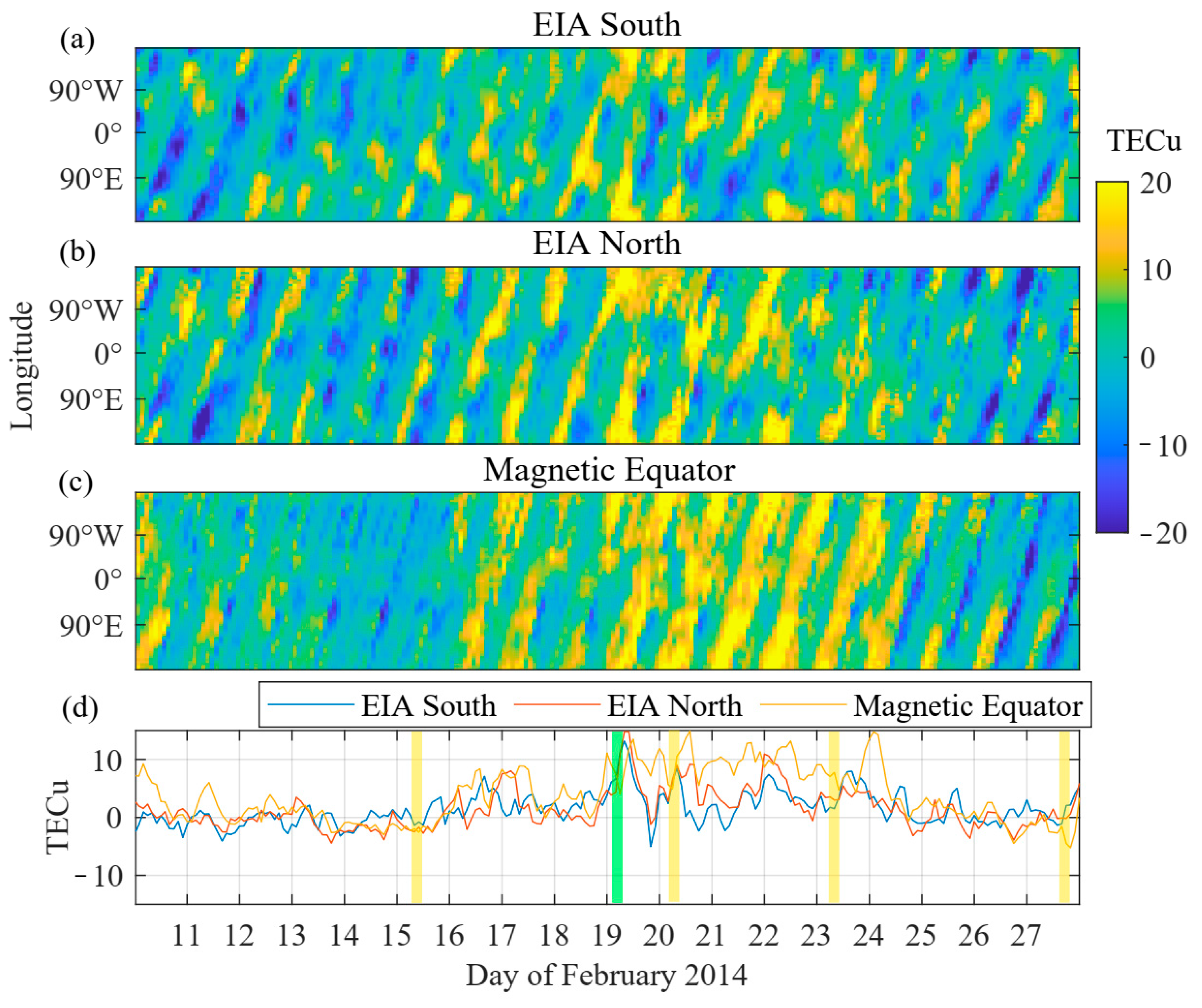
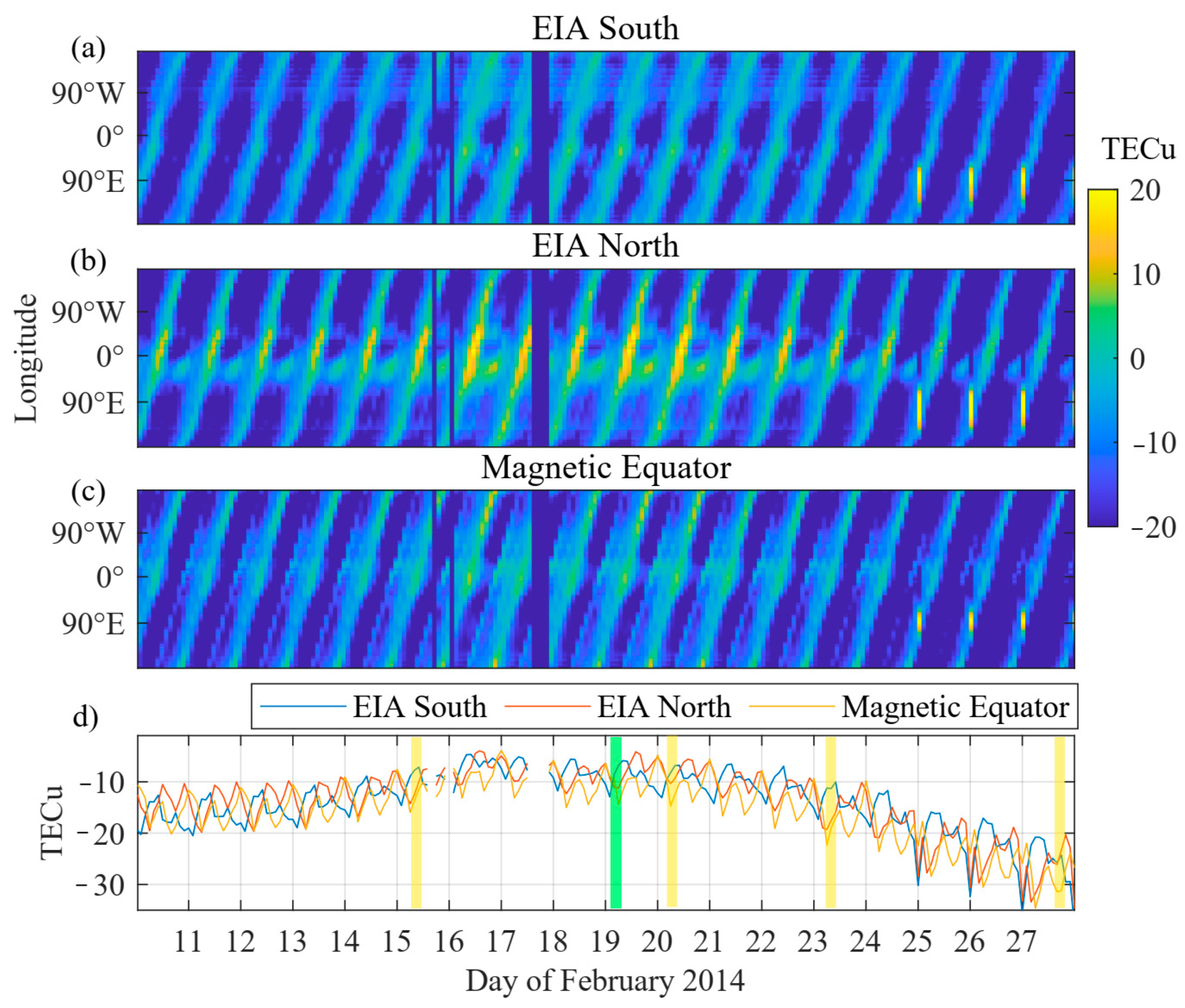
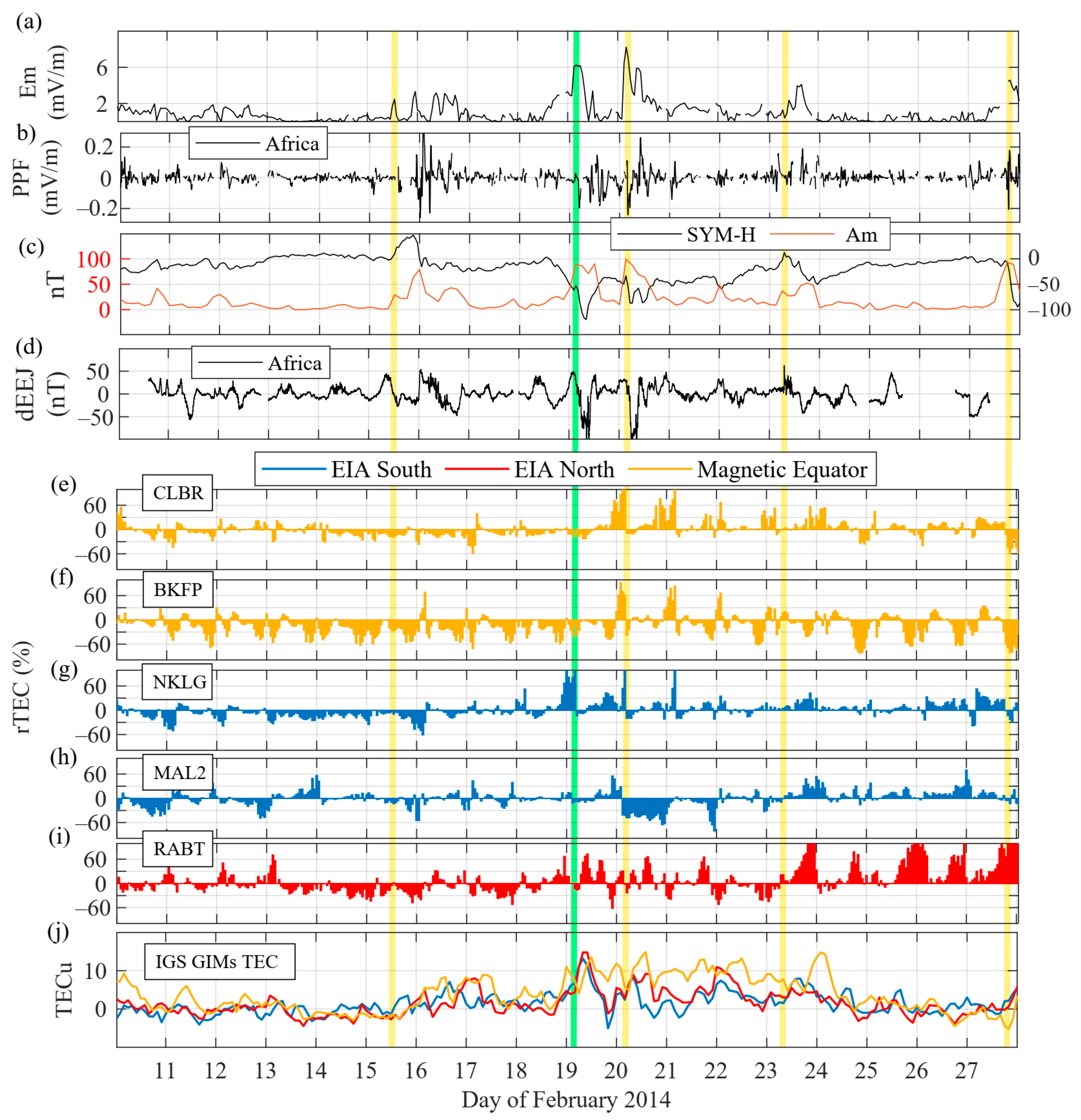
3. Results and Analyses

In February 2014, four Earth-directed coronal mass ejections (CMEs) triggered a highly complex, multiphase geomagnetic storm. The first CME arrived on 15 February, and then the other three on 19, 20, and 23 February. During this period, there were detected 11 small halo CMEs starting from the Sun (website SOHO/LASCO HALO CME catalogue, https://cdaw.gsfc.nasa.gov/CME_list/halo/halo.html, accessed date: 1 March 2021). Solar flares are classified according to their brightness intensity (I) in the X-ray wavelength range (1–8 Å): X-class (>10−4 W/m2), M-class (10−5 > I > 10−4 W/m2), C-class (10−6 > I > 10−5 W/m2), and B-class (<10−4 W/m2) flares. Since the particles travel at velocities of approximately 400 km/s, a fast gust of solar wind can take 2 to 4 days to reach Earth after it leaves the Sun. For example, two M-class flares on 12 February occurred at 6 and 16 h UT (M3.7 and M2.1, respectively), which reached Earth’s environment on 15 February, at approximately 13 h UT. On 19 February, a minor geomagnetic storm caused by the small impact on 15 February was still in progress, and the upcoming events reenergized the existing state, creating a complex multiphase storm.
Usually, geomagnetic storms begin with a sudden impulse after the arrival of an interplanetary shock (http://www.obsebre.es/en/rapid, 23 January 2022), namely a sudden storm commencement (SSC). Figure 1 shows the SSC on 15 February, which is coincident with a period of increased plasma pressure followed by peaks of southward IMF. At this point, the combination of an increased solar wind speed with the oscillation of the IMF Bz and solar wind velocity results in enhancements of Ey and Em. Subsequently, when there is solar wind pressure on the magnetosphere, variations in the geomagnetic SYM-H index result from density variations of the trapped magnetospheric particle population. In this figure, the solar wind proton density, plasma pressure, temperature, and the plasma Beta parameter, as well as the alpha/proton density ratios, are included. All these variables showed a clear variability after the SSC.
Then, the SYM-H started to decrease on 19 February at 03:00 UT. This was the starting point of a storm derived from an M1.1 CME released from the Sun on 16 February. However, the resulting storm effects lacked classical SSC characteristics. Regardless of the weak detected shock and slow decrease in SYM-H, the high-speed solar wind (HSSW) entered the magnetosphere due to the southward IMF, creating strong magnetospheric convection, which is reflected with an enhancement of the Am index up to 92 nT (similar to the Kp index, the Am index can be used as a proxy to evaluate the severity magnetospheric convection). Then, the SYM-H dropped down to −112 nT at 09:00 UT, and a rapid northward turning of the IMF resulted in a rapid recovery of SYM-H to −40 nT in approximately 12 h.
The third SSC occurred at approximately 04:00 UT on 20 February. This storm resulted from a solar filament eruption observed on 18 February (https://spaceweather.com/ accessed date: 2 February 2022) and produced a SYM-H drop from −40 nT down to −86 nT at 12:00 UT on 20 February. The SYM-H index recovered rapidly up to −40 nT at 19:00 UT and then gradually increased to 4 nT until the onset of the fourth storm at 08:00 UT on 23 February, followed by a minimum of −56 nT at 00:00 UT on 24 February. This slow-moving M3.0 CME was ejected from the Sun on 20 February. Finally, we can observe one more storm that began at 16:00 UT on 27 February, showing a minimum SYM-H of −99 nT at 00:00 UT on 28 February. Due to the isolated character of this last storm, it was not investigated.
The TEC responses were investigated with the analysis of data from permanent GNSS stations located at similar geomagnetic longitudes and at slightly shifted latitudes in the equatorial region of Africa. Figure 2 shows the effects of the multiphase storms on the low latitude ionosphere of the Africa sector and the GNSS TEC and rTEC change for the MAL2, NKLG, BKFP, RABT, and CLBR stations. The locations of these stations are shown in Table 1. The TEC diurnal variation shows the characteristic pre-dawn minimum followed by an early morning increase that reaches a maximum after noon, with TEC values between 40 and 70 TECU with respect to the night side, depending on the station. Then, clear rTEC enhancements above 60% appeared during the HSSW on 19 February at NKLG. The TEC responses from these stations are highly different and show complex patterns.
On the SSC of 20 February, the MAL2 indicates a clear depletion, whereas, at the same time, the other stations show enhanced rTEC above 60%. TEC disturbances (|rTEC| ≥ 30%) dominate during the main-phase periods and may be related to thermospheric neutral winds propagating to low latitudes. Note also MAL2 shows a large depletion on 20 February and a second peak on 21 February in the night side. The TEC variations at NKLG and CLBR stations are 24 h delayed in the enhancements at the night side from 20 to 24 February, showing an EIA expansion to lower latitudes; both stations are located in the southern hemisphere but separated by approximately 4 degrees in latitude. However, the TEC variations at BKFP (also located at the southern hemisphere) show TEC depletions at the night side during the analyzed period, which turn to positive enhancements from 20 to 24 February, following a similar pattern to that seen at CLBR. The TEC variations at the RABT station show enhancements from 19 to 22 February at the noon side, and very prompt enhancements are seen after 23 February, showing a clear drift to higher latitudes.
The EEJ and PPEF vary significantly after the SSCs and HSSW for all the events in all the longitudinal sectors (Figure 3 and Figure 4). In Figure 4, the evening peak in PPEF corresponds to the pre-reversal enhancement of the eastward electric field near sunset, which is at the origin of the peak in TEC at MAL2 (Figure 2). The most significant EEJ perturbations occurred in the African sector during the main phase of the storm on 19 to 20 February, with values below 50 nT. At this point, the effect of the disturbance dynamo clearly produces a reversed EEJ. The EEJ varied mostly in the American and African sectors during the main phase of the 19 to 20 February geomagnetic storm. Minor EEJ variability is seen in the Asian sector, probably due to the lower fluctuation captured by the experiment, although the PPEF perturbations are very prominent in all the sectors for all the SSCs and the HSSW events, with absolute values above 0.2 mV/m. The PPEF represents the transmission of the electric fields from high to low latitudes as a result of the action of the solar wind magnetosphere dynamo.
Figure 5 shows the median average of the TEC estimated by the IRI-2012 model and that from the IGS GNSS GIMs during February 2014. For both cases, there is a clear alignment of the TEC to the magnetic field, and the two characteristic enhanced EIA crests are located at about ±15° magnetic latitudes. The IRI-2012 model lacks an accurate representation of the actual median TEC during this month. The IGS GIM shows an enhanced TEC in the southern hemisphere (Figure 5b), whereas the IRI-2012 model shows lower values, providing similar TEC values for both northern and southern high latitudes (Figure 5a). Concerning the distribution of the TEC along the EIA crests, the IRI-2012 underestimates the TEC in the northern EIA crest in the African and Asian sectors and at both EIA crests in the American sector. In general, the IRI-2012 model shows narrower crests, whereas the IGS crests are wider and have a more abrupt distribution of values than that of the IRI-2012, which shows a smooth shape.
Figure 6 and Figure 7 show the keograms (time–longitudinal dependence along red lines shown in Figure 5) of the TEC near the EIA crests. Here, we remove the quiet-time TEC by setting Am = 6 in the PCA-based model of [62]. For all three datasets (IGS, IRI-2012 and PCA-based model), the profiles shown in Figure 5 (the southern and northern EIA crests and the magnetic equator) were first extracted, and the TEC differences to quiet-conditions (Am = 6) TEC from 10 to 28 February 2014 were computed. Finally, the median values of the full keogram were averaged to detect the correlations with space weather and geomagnetic indices. The averaged TEC keograms are shown in the bottom panels of Figure 6 and Figure 7, whereas the SSCs and the HSSW are shown with vertical yellow and green lines, respectively.
The differences between the keograms from IGS GIMs and the PCA-based model are shown in Figure 7. In this figure, clear responses to the different storms are seen after the SSCs and HSSW events. The PCA-based model shows a good estimation of the quiet-time TEC for this case study, showing values centered to zero TECU, i.e., TEC disturbances between 11 and 16 and 25 and 27 February are nearly zero TECU. From the residuals, there is an observation of an enhanced TEC during the storms in the Asian and American sectors (approximately at 90° W and 90° E) with respect to the African sector (0° E). The enhanced TEC appeared with the HSSW on 19 February; the TEC enhancements were over 20 TECU, and a mean value (the bottom panel) exceeded 15 TECU. The differences between the keograms of the IRI-2012 model and the IGS GIMs show smooth responses of the TEC, which covers all the storms (Figure 7). No clear distinction between the events is seen, and the African sector (0° E) seems to have an enhanced TEC with respect to the Asian and American sectors, a feature that is not accurate regarding the residuals of the IGS TEC GIMs we observe in Figure 6. In this figure, there are observations of a clear bias, approximately overestimating the actual TEC by 20 TECU.
From Figure 6, the EIA crests at both hemispheres are clearly variable during the storms, and the enhancements are very prominent in both hemispheres, immediately after the SSCs and the HSSW events, and followed by a significant variability in the main phases of the storms. The TEC enhancements in the low-latitude ionosphere on February 19 resulted from an increased merging electric field, Em. This results from the northward IMF Bz and an enhanced solar wind. Clear changes in the geomagnetic field of Earth (Figure 1i,j) are seen as the magnetosphere is compressed by the solar wind, and, for a particular orientation of IMF Bz, the magnetospheric compression can be asymmetric if there is a significant IMF Bz component. This, in turn, is reflected in the merging electric field (Em), and results in significant TEC enhancements. Figure 8 collects the results from previous figures and includes the merging electric field, Em, the geomagnetic SYM-H, Am, and Dst indices, the dPPEF, dEEJ, and rTEC variations measured by GNSS stations and magnetometers in Africa, and the GIMs TEC differences between the IGS products, as well as the quiet-time PCA-based model (Am = 6) at the EIA crests and at the magnetic equator. Colors are used to differentiate the GNSS stations in terms of proximity to the profiles, and the SSCs and HSSW are highlighted with vertical yellow and green lines, respectively.
The overall variations are most prominent during the main phase of the storm caused by the HSSW event on 19 February, followed by a complex re-energization due to the SSCs on 20 and 23 February. In these events, there is an observation of the energization in the magnetosphere–ionosphere system due to an intensified ring current, which is clearly seen by the SYM-H index (Figure 8c). Immediately after the CME arrival on 19 February at ~2 h UT, the TEC variability at the northern and southern EIA crest in Figure 8j shows very prominent enhancements of approximately 15 TECU, followed by a rapid drop to normality at the end of the day. Then, at ~3:00 UT on 20 February, a new SSC enhanced EIA crest appeared again. In the northern EIA crest, the TEC enhancements reached ~8 TECU, which lasted until the morning of 21 February, while the southern EIA crest dropped to normal values until midday of 20 February. Then, on 22 February, enhancements of ~10 and ~8 TECU appeared in the northern and the southern EIA crest, respectively, while no SSCs were observed during this period; only a small variation in Dst and AE indices was observed. Several hours after this point, on 23 February at ~7 h UT, the SSC intensified both EIA crests by ~8 TECU, with a slow recovery until 24 February at ~12:00 UT. The TEC at the magnetic equator remained intensified at approximately ~10 TECU from the beginning of the HSSW at ~2:00 UT on 19 February until ~12:00 UT on 24 February, with a sudden recovery, approximately 5 days, reaching mean values of 15 TECU at the SSC on 19 February, at the SSC on 20 February, and approximately 24 h after the SSC on 23 February.
The corresponding TEC variations from the GNSS stations (Figure 8e–i) follow similar patterns of TEC variability, with clear differences, most probably caused by local irregularities, where plasma is differently distributed during the different phases of the storms as compared to the averaged character of the IGS TEC. For the northern EIA crest, the rTEC enhancements exceeded 60% at the NKLG station on 19 February, which clearly coincides with the responses of the IGS TEC. This is also slightly appreciable in the southern EIA crest for the RABT station. Moreover, on the SSC event of 20 February, a clear enhancement appeared at both GNSS stations in the dip equator region (CLBR and BKFP); this corresponded with the response of the IGS profile. Here, there was an observation of the depletion after the rapid recovery in the MAL2 station, which matches with the low TEC values of the southern IGS profile. On the contrary, at the dip equatorial region on 20 February, the CLBR and BKFP GNSS stations showed clear enhancements following a long period of an enhanced TEC at the IGS profile, which lasted with several peaks until 24 February.
The variability in the merging electric field Em is associated with the variability in the PPEF (Figure 8b), mostly for all the SSCs and the HSSW events during the main phases of the storms. Although the storm on 20 February was stronger than that on 15 February, these featured a similar PPEF variation, with amplitudes of approximately 0.25 mV/m. However, the EEJ illustrated maximal development starting from the SSC along the storm main phase (Figure 8d). The EEJ largely varied during 19 and 20 February, with less intensity the rest of the period, reaching values of −100 nT, and with an amplitude of 150 nT during ~12 h after the SSCs. This is the effect of the disturbance dynamo. At the beginning of the storm, there was only PPEF at the equator, and, after several hours, the DDEF was acting at the equator.
Figure 9 shows a global perspective of the magnetosphere–ionosphere variations caused by the multiphase storm of February 2014. The ASY-D and ASY-H indices correlate with the Am index (Figure 9b). The GEC index shows the dynamics of the ionosphere as a whole during the storms [56]. This figure also includes the current Intensity CI variations at the different regions (Figure 9c,d) and the total CI (Figure 9e). Finally, the IGS TEC profiles are shown at the bottom of this figure. All the global variables shown in Figure 9 reflect the SSCs and HSSW events. All the variables peaked at 0:00 UT on 16 February. Subsequently, TEC enhancements appeared in the IGS profiles from 16 to 18 February. The HSSW on 19 February accompanied a CI increase (~150 kA) in the American sector at 0:00 UT, probably due to enhanced currents near the South Atlantic Anomaly. At this time, the GEC also showed an enhancement of approximately 0.2 GECU. The maximal CI enhancement over 300 kA (appeared during the SSC of 23 February in the Asian sector) accompanied the lowest SYM-H values. Note that, during an SSC, there is a compression in front of the magnetosphere, and the resulting magnetopause current creates the magnetic variations observed at the ground level; these magnetic variations were used to compute the ionospheric currents. From this point, the GEC index shows a gradual increase up to 3.5 GECU at the end of the month, showing the ionospheric response to the complex processes of long-duration energization during this complex multiphase geomagnetic storm. For the final observation, there was increased CI at the African Sector, more prominent in the Northern hemisphere, which indicates the responses to the upcoming SSC at the end of the month.

4. Discussion

Ionospheric perturbations following geomagnetic storms are caused by solar wind shockwaves that interact with Earth’s magnetosphere, causing magnetic field disturbances and subsequent TEC variations that last from several hours to several days [64]. TEC variability is linked to several physical and chemical phenomena, including chemistry, ambipolar diffusion, transport due to E × B drift, and transport due to neutral wind (e.g., [65,66]).
During the second half of February 2014, four M-class CMEs caused three clear SSCs on 15, 20, and 23 February, and one HSSW event on 19 February with the absence of classical SSC features. The magnetospheric reaction to the HSSW on 19 February resulted in an SYM-H peak of −112 nT. For the HSSW storm, no classical SSC is seen, most probably due to the prevalent magnetospheric convection caused by the preceding southward IMF on 15 February.
Negative IMF Bz and increased solar wind pressure resulted in an increased merging electric field Em, and thus intensified the magnetospheric convection (reflected by the Am index). Low-latitude TEC enhancements resulting from the HSSW on 19 February reached over 20 TECU in the IGS profiles, and these were longer-lasting at the dip equator than in the EIA crests along the successive SSCs events on 20 and 23 February. From this point, the observations were of a gradual increase in GEC up to 3.5 GECU at the end of the month, showing 1 GECU differential intensification. This increase was not reflected by the low-latitude IGS TEC profiles (Figure 9g), but clear rTEC enhancements over 60% were observed during the same period on the night side at the RABT ground station. This increased gradient may be localized at higher latitudes following the EIA expansion generated by the day-time eastward electric fields causing E × B vertical plasma uplift.
All the GNSS stations showed irregular TEC variability due to the EIA expansion towards mid-latitudes. Day- and night-side TEC enhancements were observed as plasma flowed along the magnetic field lines to the mid- and high latitudes [67]. It is clear that the low-latitude TEC variability is strongly influenced by the storm-time EIA expansion, as shown by, e.g., Ref. [68].
The ionospheric TEC disturbances in the African sector differed significantly at stations located at different magnetic latitudes. The TEC depletion at the dip equator could be due to the enhancement of the fountain effect. The observed TEC variations respond to energy injection at storm onset [69], which also depends on thermospheric chemistry processes. We consider the E × B drift disturbance to be the main contribution of the observed TEC variability. DDEF phenomena and PPEF processes change the E × B drift and its effect; the change depends on magnetic latitude nonlinearly [70]. The PPEF plays an important role in the ionosphere processes at the equatorial regions during geomagnetic storms, whereas [71,72] provided similar conclusions.
We suspect that EIA expansion may be produced by eastward PPEF in the Asian sector, where the main phase of the geomagnetic storms occurred at the day side. The post-sunset PPEF of the eastward (daytime) and westward (nighttime) drifts combine to drag plasma from the dip equator by E × B convection, sustaining the plasma pile at the EIA crests. The polarity of the PPEF was eastward and westward during day- and night- time, respectively ([40], and references therein), while, during day-side and post-sunset, it has eastward polarity intensified through plasma induction at the EIA crest. The EEJ data show that the storm-time PPEFs are an important contribution of the observed ionospheric responses to this multiphase geomagnetic storm.
Contributions of neutral winds should also be considered and investigated from, for example, LEO satellites (e.g., thermospheric winds estimated from accelerometers [73,74] onboard Swarm, Gravity Recovery and Climate Experiment, etc.) and other sources in the future. The low-latitude PPEF mechanism is mainly driven by tidal wind through the DDEF effect, where wind increases with increasing latitude, and the tidal wind is modulated by planetary waves.

5. Conclusions

In February 2014, the Sun produced eleven small halo CMEs, including four powerful Earth-directed CMEs that triggered a multiphase geomagnetic storm. The first CME (generated two M-class flares on 12 February) arrived to Earth on 15 February and caused a minor geomagnetic storm. On 19 February, the prevalent minor G-1 geomagnetic storm was still in the recovery phase when a sudden HSSW event reenergized the existing disturbances, causing a complex moderate G-2 geomagnetic storm. Two more SSC events on 20 and 23 February 2014 made the storm highly complex. In this work, the low-latitude ionosphere responses and coupling mechanisms of this complex multiphase geomagnetic storm are investigated using space weather indices, magnetometers, and TEC data from ground-based GNSS stations, and ionospheric empirical models. The main conclusions from our analyses are as follows:
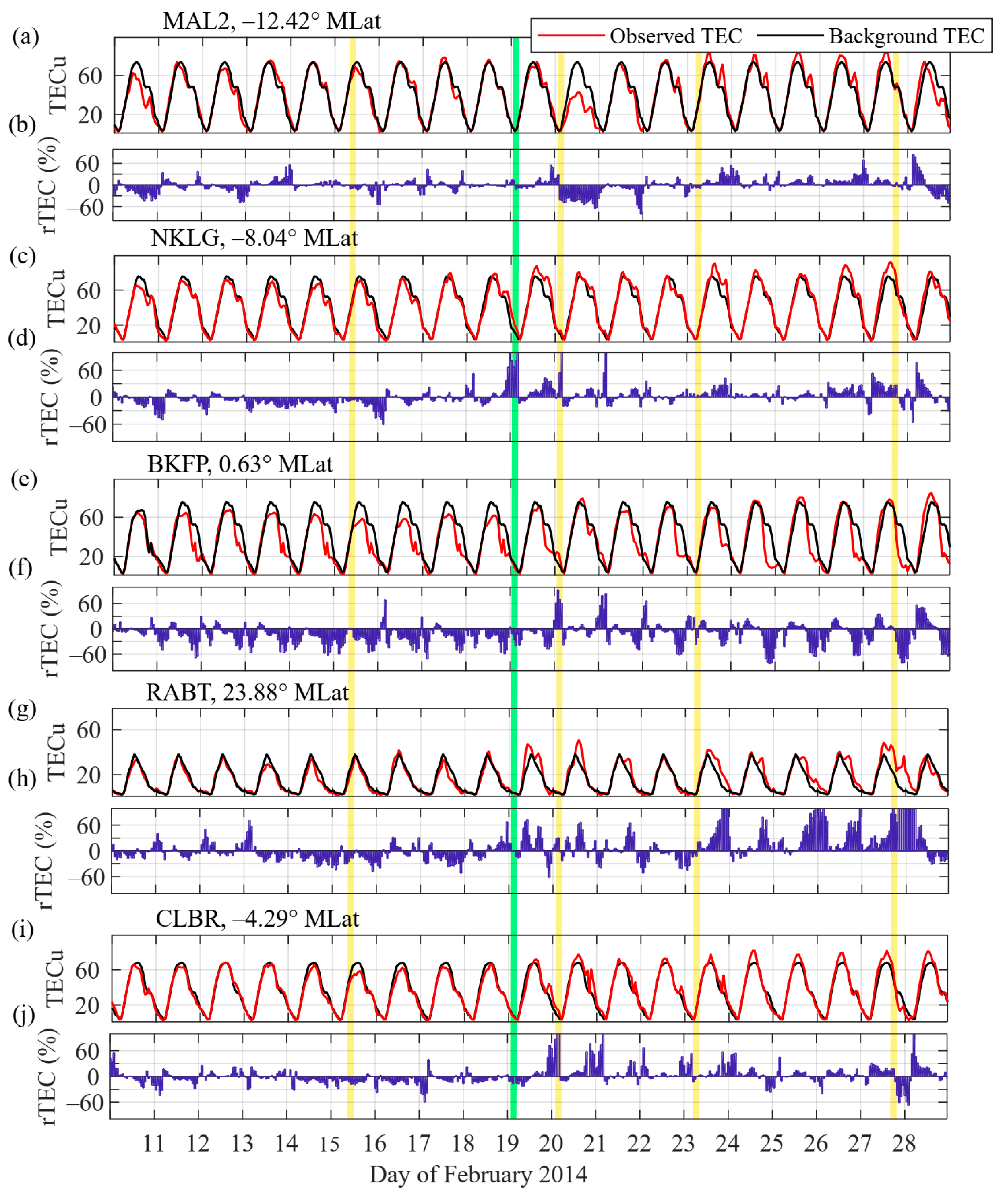
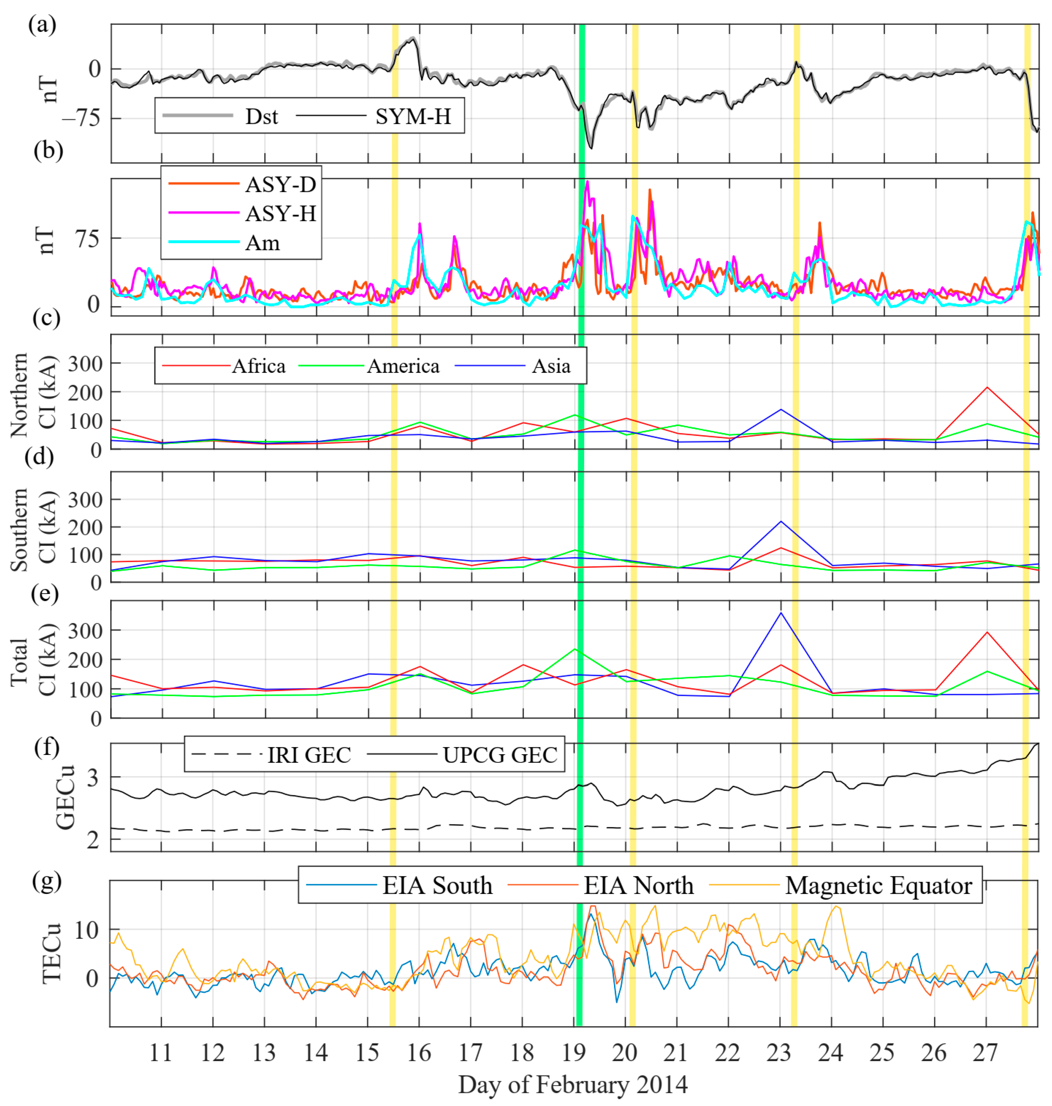
  • Clear TEC depletions/enhancements were observed at the GNSS stations used in this study, and TEC enhancements from the IGS GIMs are up to 20 TECU, lasting from 16 to 18 February 2014. A delay in TEC enhancements towards high-latitude stations was observed, which is attributed to the EIA expansion. TEC enhancements up to 20 TECU have been at low-latitudes with longer-lasting TEC enhancements at the dip equator (from 16 to 18 February) rather than in the EIA crests (only after the CMEs arrivals).
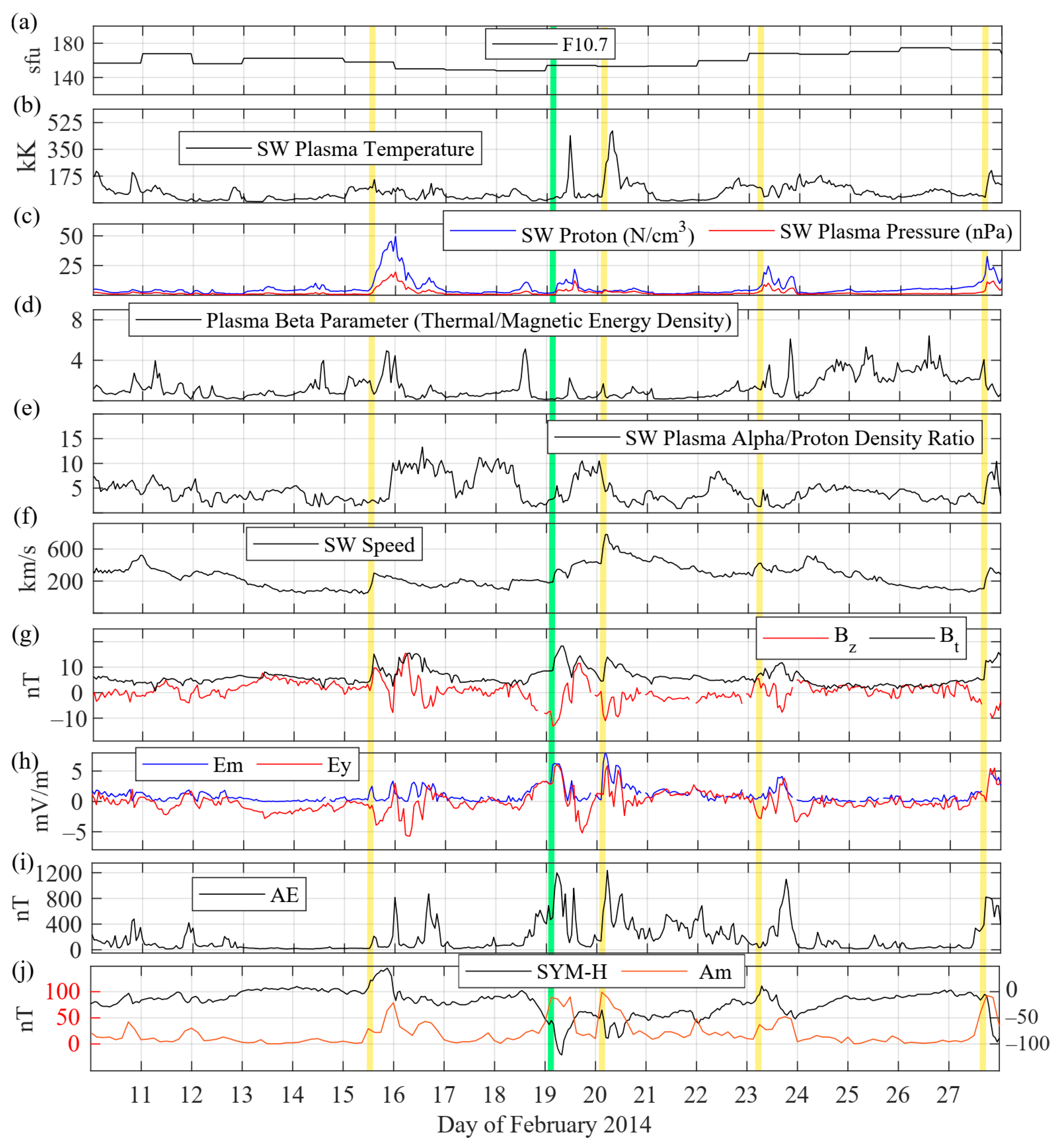
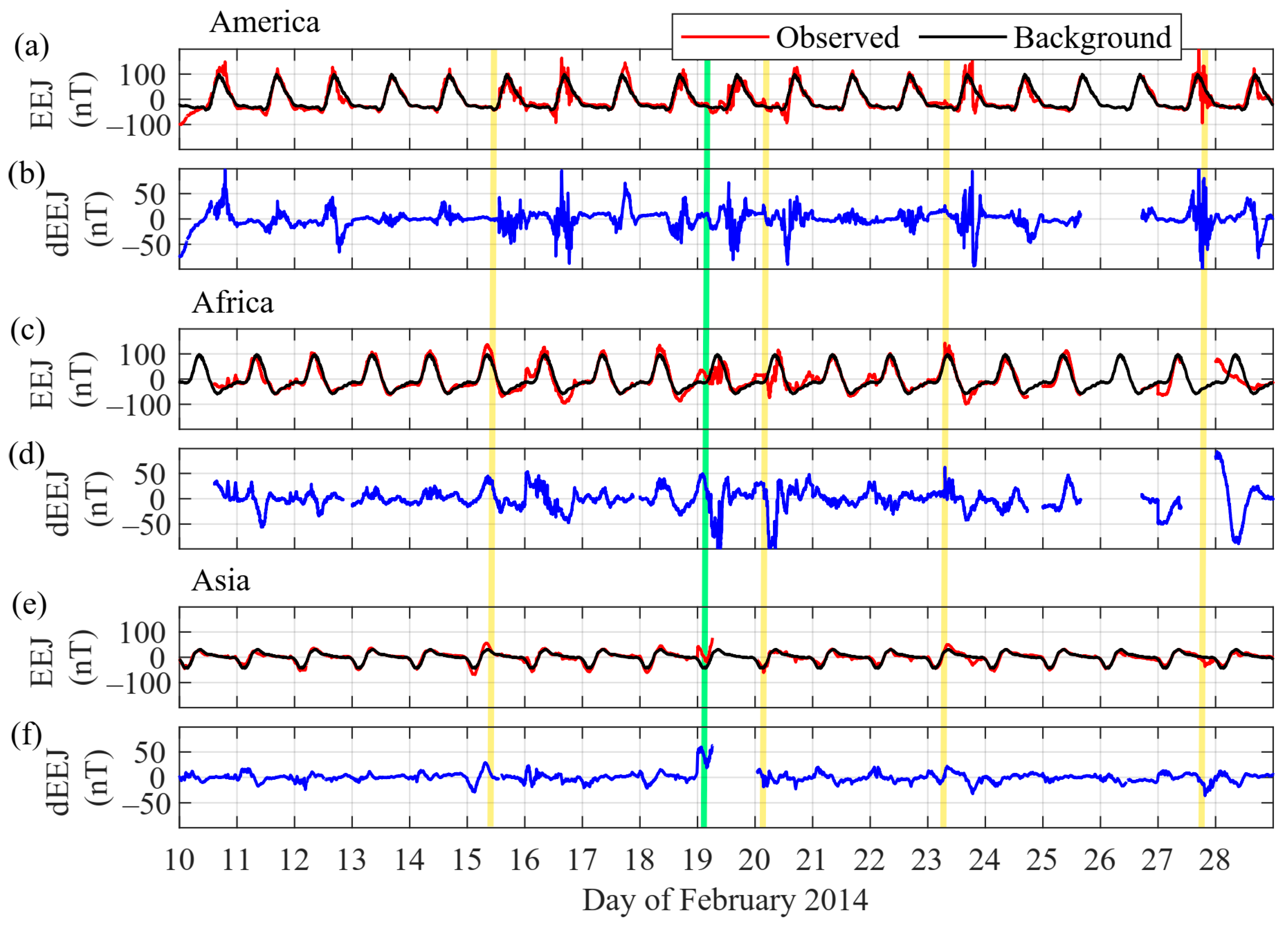
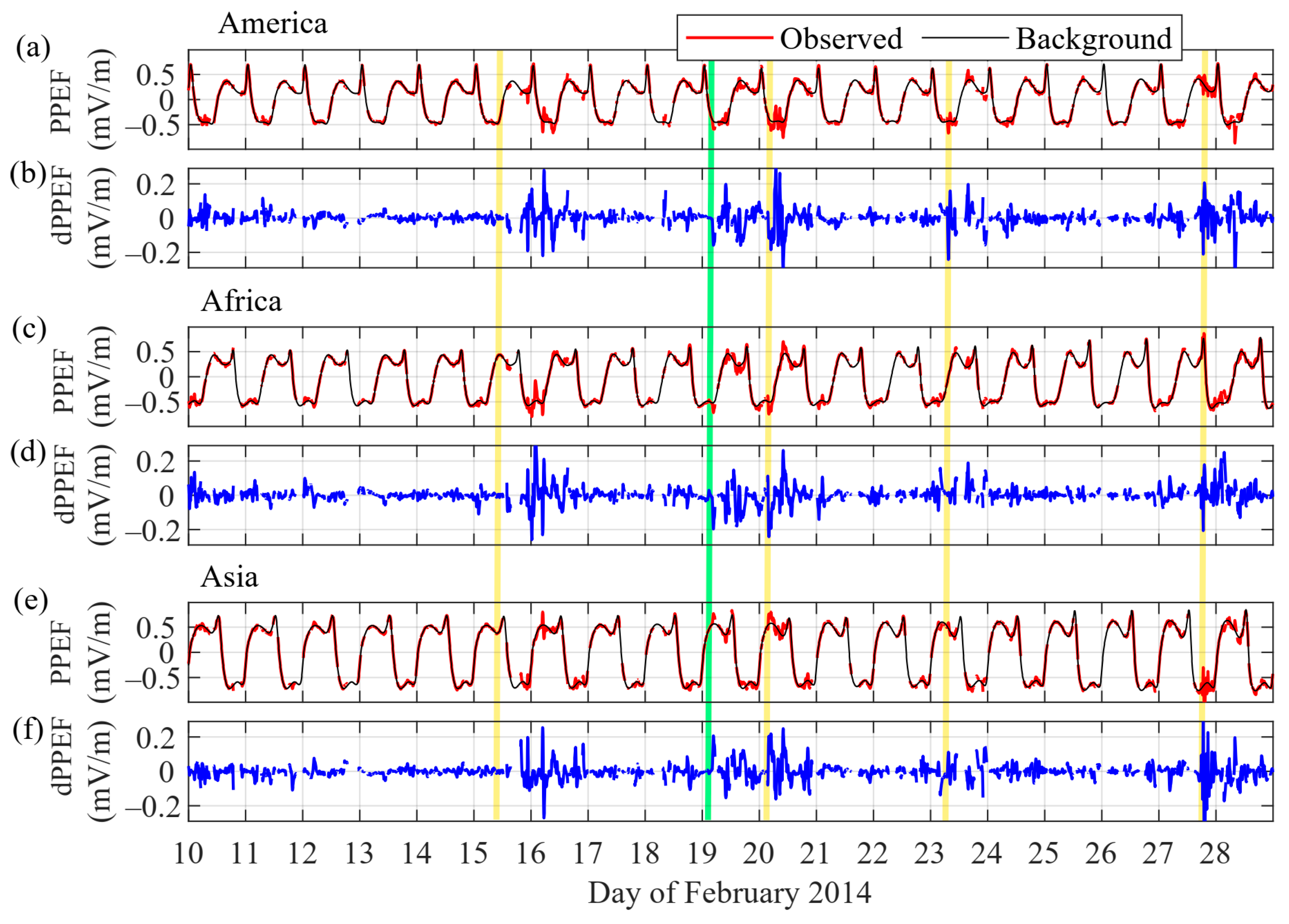
  • Rapidly after the arrival of each CME, PPEF disturbances with amplitudes of 0.4 mV/m have been observed in the American, African, and Asian sectors. The EEJ variations exceeded amplitudes of 100 nT with the exception of the Asian region, which has shown minimal EEJ variability.
  • The HSSW event on 19 February seems to have reenergized the existing storm conditions (CME arrival of 15 February) and subsequently caused a moderate G-2 geomagnetic storm, which was further enhanced by two more SSC events on 20 and 23 February. The prevalent magnetospheric convection caused by the preceding southward IMF on 19 February was the cause of no classical SSC. From the HSSW event, there has been the observation of a gradual increase in GEC up to 3.5 GECU at the end of the month, showing approximately 1 GECU of differential intensification. This gradient is not reflected by the IGS-derived TEC profiles, but clear rTEC enhancements over 60% during the same period at the RABT GNSS ground station were noticed, suggesting this enhanced TEC to be located at higher latitudes.
  • The IRI-2012 model did not represent the actual TEC variability during the storms period, showing no distinction between events, and a clear bias of ~20 TECU to the actual quiet-time TEC. There was also a detection of a clear discrepancy in the distribution of TEC along the EIA, showing that IRI-2012 underestimates the northern crest at the African and Asian sectors and at both crests in the American sector. The median February average from the IGS GIM TEC shows enhanced values in the southern hemisphere, whereas the IRI-2012 does not show this asymmetry.

Author Contributions

Investigation, data curation, visualization, writing—original draft preparation, A.C., C.A., M.S., Y.Y. and C.O.; conceptualization, formal analysis, supervision, writing—review and editing, A.C., C.A.-M. and S.J.; funding acquisition, S.J. All authors have read and agreed to the published version of the manuscript.

Funding

This research was partly funded by: (S.J.) the National Natural Science Foundation of China (NSFC) Project (Grant No. 12073012), Nanjing, China; (A.C.) the Talent Start-Up Funding project of NUIST (Grant No. 1411041901010), Nanjing, China; (A.C.) the Giner de los Ríos Grant of University of Alcalá, Madrid, Spain; and (Y.Y.) the Ministry of Science and Higher Education of the Russian Federation, Irkutsk, Russia.

Institutional Review Board Statement

Not applicable.

Informed Consent Statement

Not applicable.

Data Availability Statement

Not applicable.

Acknowledgments

This study is an outcome of the Joint Study Group 1: ’Coupling processes between magnetosphere, thermosphere, and ionosphere’ of the International Association of Geodesy Global Geodetic Observing System Focus Area Geodetic Space Weather Research, Vienna, Austria (https://ggos.org/about/org/fa/geodetic-space-weather-research/groups/jsg1-coupling-processes/, accessed on 15 February 2022). The space weather indices are available at the NASA OMNI website (http://omniweb.gsfc.nasa.gov/, accessed on 15 February 2022) and at the ISGI website (http://isgi.unistra.fr, accessed on 15 February 2022). The magnetometer data are available at the UCB website (http://geomag.colorado.edu, accessed on 15 February 2022). The sTEC data used in this study are available at the AFREF website (http://afrefdata.org, accessed on 15 February 2022), and the IGS GIMs TEC are available at the IRI-MODEL website (https://irimodel.org/, accessed on 15 February 2022). The IRI-2012 model is available at the CCMC website (https://ccmc.gsfc.nasa.gov, accessed on 15 February 2022), and the PCA-based TEC model by [62] is available in [63] at the Zenodo repository (https://zenodo.org/record/3563463, accessed on 15 February 2022). Special thanks are given to Catherine M Jones and to the anonymous reviewers for helping to improve the manuscript.

Conflicts of Interest

The authors declare no conflict of interest.

References

  1. Hernández-Pajares, M.; Juan, J.; Sanz, J. New approaches in global ionospheric determination using ground GPS data. J. Atmos. Sol. Terr. Phys. 1999, 61, 1237–1247. [Google Scholar] [CrossRef]
  2. Jin, S.G.; Su, K. PPP models and performances from single- to quad-frequency BDS observations. Satell. Nav. 2020, 1, 16. [Google Scholar] [CrossRef]
  3. Afraimovich, E.L.; Astafyeva, E.I.; Demyanov, V.V.; Edemskiy, I.K.; Gavrilyuk, N.S.; Ishin, A.B.; Kosogorov, E.A.; Leonovich, L.A.; Lesyuta, O.S.; Perevalova, N.P.; et al. Review of GPS/GLONASS studies of the ionospheric response to natural and anthropogenic processes and phenomena. J. Space Weather Space Clim. 2013, 3, A27. [Google Scholar] [CrossRef] [Green Version]
  4. Jin, S.; Jin, R.; Kutoglu, H. Positive and negative ionospheric responses to the March 2015 geomagnetic storm from BDS observations. J. Geod. 2017, 91, 613–626. [Google Scholar] [CrossRef]
  5. Gao, C.; Jin, S.; Yuan, L. Ionospheric responses to the June 2015 geomagnetic storm from ground and LEO GNSS observations. Remote Sens. 2020, 12, 2200. [Google Scholar] [CrossRef]
  6. Ratovsky, K.G.; Klimenko, M.V.; Dmitriev, A.V.; Medvedeva, I.V. Relation of Extreme Ionospheric Events with Geomagnetic and Meteorological Activity. Atmosphere 2022, 13, 146. [Google Scholar] [CrossRef]
  7. Klobuchar, J.A. Ionospheric time-delay algorithm for single-frequency GPS users. IEEE Trans. Aerosp. Electron. Syst. 1987, 23, 325–331. [Google Scholar] [CrossRef]
  8. Huba, J.D.; Joyce, G.; Fedder, J.A. Sami2 is Another Model of the Ionosphere (SAMI2): A new low-latitude ionosphere model. J. Geophys. Res. Atmos. 2000, 105, 23035–23053. [Google Scholar] [CrossRef]
  9. Hoque, M.M.; Jakowski, N.; Berdermann, J. Ionospheric correction using NTCM driven by GPS Klobuchar coefficients for GNSS applications. GPS Solut. 2017, 21, 1563–1572. [Google Scholar] [CrossRef]
  10. Radicella, S. The NeQuick model genesis, uses and evolution. Ann. Geophys. 2009, 52, 417–422. [Google Scholar] [CrossRef]
  11. Okoh, D.; Onwuneme, S.; Seemala, G.; Jin, S.G.; Rabiu, B.; Nava, B.; Uwamahoro, J. Assessment of the NeQuick-2 and IRI-Plas 2017 models using global and long-term GNSS measurements. J. Atmos. Sol. Terr. Phys. 2018, 170, 1–10. [Google Scholar] [CrossRef]
  12. Bilitza, D. IRI the International Standard for the Ionosphere. Adv. Radio Sci. 2018, 16, 1–11. [Google Scholar] [CrossRef] [Green Version]
  13. Fuller Rowell, T.J. Stormtime response of the thermosphereionosphere system. In Aeronomy of the Earth’s Atmosphere and Ionosphere; Abdu, M.A., Pancheva, D., Bhattacharyya, A., Eds.; IAGA Spec. Sopron Book Series; Springer: Dordrecht, The Netherlands, 2011; Chapter 32; Volume 2, p. 419435. [Google Scholar] [CrossRef]
  14. Calabia, A.; Jin, S. Characterization of the Upper Atmosphere from Neutral and Electron Density Observations. In International Association of Geodesy Symposia; Springer: Berlin/Heidelberg, Germany, 2020. [Google Scholar] [CrossRef]
  15. Astafyeva, E.; Bagiya, M.S.; Förster, M.; Nishitani, N. Unprecedented Hemispheric Asymmetries During a Surprise Ionospheric Storm: A Game of Drivers. J. Geophys. Res. Space Phys. 2020, 125, e2019JA027261. [Google Scholar] [CrossRef]
  16. Shah, M.; Abbas, A.; Ehsan, M.; Calabia, A.; Adhikari, B.; Tariq, M.A.; Ahmed, J.; de Oliveira-Junior, J.F.; Yan, J.; Melgarejo-Morales, A.; et al. Ionospheric-Thermospheric Responses to the August 2018 Geomagnetic Storm over South America from Multiple observable. IEEE J. Sel. Top. Appl. Earth Obs. Remote Sens. 2022, 15, 261–269. [Google Scholar] [CrossRef]
  17. Cai, X.; Burns, A.G.; Wang, W.; Qian, L.; Solomon, S.C.; Eastes, R.W.; McClintock, W.E.; Laskar, F.I. Isnvestigation of a neutral “tongue” observed by GOLD during the geomagnetic storm on 11 May 2019. J. Geophys. Res. Space Phys. 2021, 126, e2020JA028817. [Google Scholar] [CrossRef]
  18. Jin, S.G.; Gao, C.; Yuan, L.; Guo, P.; Calabia, A.; Ruan, H.; Luo, P. Long-term variations of plasmaspheric total electron content from topside GPS observations on LEO satellites. Remote Sens. 2021, 13, 545. [Google Scholar] [CrossRef]
  19. Calabia, A.; Jin, S. Solar cycle, seasonal, and asymmetric dependencies of thermospheric mass density disturbances due to magnetospheric forcing. Ann. Geophys. 2019, 37, 989–1003. [Google Scholar] [CrossRef] [Green Version]
  20. Calabia, A.; Jin, S. Thermospheric mass density disturbances due to magnetospheric forcing from 2014–2020 CASSIOPE precise orbits. J. Geophys. Res. Space Phys. 2021, 126, e2021JA029540. [Google Scholar] [CrossRef]
  21. Namba, S.; Maeda, K.-I. Radio Wave Propagation; Corona Publishing: Tokyo, Japan, 1939; 86p. [Google Scholar]
  22. Appleton, E. Two anomalies in the ionosphere. Nature 1946, 693, 57–69. [Google Scholar] [CrossRef]
  23. Chapman, S. The equatorial electrojet as detected from the abnormal electric current distribution above Huancayo Peru, and elsewhere. Arch Meteorol. Geophys. U Bioklimatol. Ser. 1951, 4, 368–374. [Google Scholar] [CrossRef]
  24. Takeda, M. Contribution of wind, conductivity, and geomagnetic main field to the variation in the geomagnetic Sq field. J. Geophys. Res. Space Phys. 2013, 118, 4516–4522. [Google Scholar] [CrossRef]
  25. Basu, S.; Basu, S. Equatorial scintillations, a review. J. Atmos. Terr. Phys. 1981, 43, 473–478. [Google Scholar] [CrossRef]
  26. Kelley, M.C. The Earth Ionosphere; Elsevier Press: Amsterdam, The Netherlands; Academic Press: San Diego, CA, USA, 1989. [Google Scholar]
  27. Fejer, B.G.; de Paula, E.R.; González, S.A.; Woodman, R.F. Average vertical and zonal F region drifts over Jicamarca. J. Geophys. Res. Space Phys. 1991, 96, 13901–13906. [Google Scholar] [CrossRef] [Green Version]
  28. Vasyliunas, V.M. Mathematical models of the magnetospheric convection and its coupling to the ionosphere. In Particles and Fields in the Magnetosphere; McCormac, M., Ed.; Springer: New York, NY, USA, 1970. [Google Scholar] [CrossRef]
  29. Fuller-Rowell, T.J.; Codrescu, M.V.; Moffett, R.J.; Quegan, S. Response of the thermosphere and ionosphere to geomagnetic storms. J. Geophys. Res. Space Phys. 1994, 99, 3893–3914. [Google Scholar] [CrossRef]
  30. Blanc, M.; Richmond, A.D. The ionospheric disturbance dynamo. J. Geophys. Res. Space Phys. 1980, 85, 1669. [Google Scholar] [CrossRef]
  31. Fejer, B.G.; Larsen, M.F.; Farley, D.T. Equatorial disturbance dynamo electric fields. Geophys. Res. Lett. 1983, 10, 537–540. [Google Scholar] [CrossRef]
  32. Jacobsen, K.S.; Dähnn, M. Statistics of ionospheric disturbances and their correlation with GNSS positioning errors at high latitudes. J. Space Weather. Space Clim. 2014, 4, A27. [Google Scholar] [CrossRef] [Green Version]
  33. Jakowski, N.; Béniguel, Y.; de Franceschi, G.; Pajares, M.H.; Jacobsen, K.S.; Stanislawska, I.; Tomasik, L.; Warnant, R.; Wautelet, G. Monitoring, tracking and forecasting ionospheric perturbations using GNSS techniques. J. Space Weather. Space Clim. 2012, 2, A22. [Google Scholar] [CrossRef] [Green Version]
  34. Wang, W.; Lei, J.; Burns, A.G.; Solomon, S.C.; Wiltberger, M.; Xu, J.; Zhang, Y.; Paxton, L.; Coster, A. Ionospheric response to the initial phase of geomagnetic storms: Common features. J. Geophys. Res. Space Phys. 2010, 115, A07321. [Google Scholar] [CrossRef]
  35. Lei, J.; Wang, W.; Burns, A.G.; Solomon, S.C.; Richmond, A.D.; Wiltberger, M.; Goncharenko, L.P.; Coster, A.; Reinisch, B.W. Observations and simulations of the ionospheric and thermospheric response to the December 2006 geomagnetic storm: Initial phase. J. Geophys. Res. Space Phys. 2008, 113, A01314. [Google Scholar] [CrossRef]
  36. Sahai, Y.; Fagundes, P.R.; Becker-Guedes, F.; Bolzan, M.J.A.; Abalde, J.R.; Gil Pillat, V.; De Jesus, R.; Lima, W.L.C.; Crowley, G.; Shiokawa, K.; et al. Effects of the major geomagnetic storms of October 2003 on the equatorial and low latitude F region in two longitudinal sectors. J. Geophys. Res. Space Phys. 2005, 110, A12S91. [Google Scholar] [CrossRef]
  37. Kuai, J.; Liu, L.; Liu, J.; Zhao, B.; Chen, Y.; Le, H.; Wan, W. The long-duration positive storm effects in the equatorial ionosphere over Jicamarca. J. Geophys. Res. Space Phys. 2015, 120, 1311–1324. [Google Scholar] [CrossRef]
  38. Heelis, R.A. Electrodynamics in the low and middle latitude ionosphere: A tutorial. J. Atmos. Sol. Terr. Phys. 2004, 66, 825–838. [Google Scholar] [CrossRef]
  39. Pedatella, N.M.; Forbes, J.M.; Lei, J.; Thayer, J.P.; Larson, K.M. Changes in the longitudinal structure of the low latitude ionosphere during the July 2004 sequence of geomagnetic storms. J. Geophys. Res. Space Phys. 2008, 113, A11315. [Google Scholar] [CrossRef] [Green Version]
  40. Astafyeva, E.; Yasyukevich, Y.V.; Maletckii, B.; Oinats, A.; Vesnin, A.; Yasyukevich, A.S.; Syrovatskii, S.; Guendouz, N. Ionospheric Disturbances and Irregularities during the 25–26 August 2018 Geomagnetic Storm. J. Geophys. Res. Space Phys. 2022, 127, e2021JA029843. [Google Scholar] [CrossRef]
  41. Mansilla, G.A.; Zossi, M.M. Longitudinal Variation of the Ionospheric Response to the 26 August 2018 Geomagnetic Storm at Equatorial/Low Latitudes. Pure Appl. Geophys. 2020, 177, 5833–5844. [Google Scholar] [CrossRef]
  42. Kutiev, I.; Watanabe, S.; Otsuka, Y.; Saito, A. Total electron content behavior over Japan during geomagnetic storms. J. Geophys. Res. Space Phys. 2005, 110, A01308. [Google Scholar] [CrossRef] [Green Version]
  43. Ghamry, E.; Lethy, A.; Arafa-Hamed, T.; Elaal, E.A. A comprehensive analysis of the geomagnetic storms occurred during 18 February and 2 March 2014. NRIAG J. Astron. Geophys. 2016, 5, 263–268. [Google Scholar] [CrossRef] [Green Version]
  44. King, J.H.; Papitashvili, N.E. Solar wind spatial scales in and comparisons of hourly Wind and ACE plasma and magnetic field data. J. Geophys. Res. 2005, 110, A02209. [Google Scholar] [CrossRef]
  45. Mayaud, P.N. Derivation, Meaning, and Use of Geomagnetic Indices; Geophysical Monograph Series; AGU: Washington, DC, USA, 1980; Volume 22. [Google Scholar]
  46. Liu, R.; Lühr, H.; Doornbos, E.; Ma, S.-Y. Thermospheric mass density variations during geomagnetic storms and a prediction model based on the merging electric field. Ann. Geophys. 2010, 28, 1633–1645. [Google Scholar] [CrossRef] [Green Version]
  47. Kan, J.K.; Lee, L.C. Energy coupling function and solar wind-magnetosphere dynamo. Geophys. Res. Lett. 1979, 6, 577–580. [Google Scholar] [CrossRef]
  48. Gurtner, W.; Estey, L. RINEX: The Receiver Independent Exchange Format Version 3.00. 20. Available online: https://files.igs.org/pub/data/format/rinex300.pdf (accessed on 6 February 2022).
  49. Peymirat, C.; Richmond, A.D.; Kobea, A.T. Electrodynamic coupling of high and low latitudes: Simulations of shielding and overshielding effects. J. Geophys. Res. Space Phys. 2000, 105, 22991–23003. [Google Scholar] [CrossRef]
  50. Manoj, C.; Maus, S.; Lühr, H.; Alken, P. Long-period prompt-penetration electric fields derived from CHAMP satellite Magnetic Measurements. J. Geophys. Res. Space Phys. 2013, 118, 5919–5930. [Google Scholar] [CrossRef] [Green Version]
  51. Vasyliunas, V.M. The interrelationship of magnetospheric processes. In Earth’s Magnetosphere Processes; McCormac, M., Ed.; D. Reidel: Norwell, MA, USA, 1972; pp. 29–38. [Google Scholar]
  52. Kobéa, A.T.; Richmond, A.D.; Emery, B.A.; Peymirat, C.; Luhr, H.; Moretto, T.; Hairston, M.; Amory-Mazaudier, C. Electrodynamic Coupling of High and Low Latitudes Observations on 27 May 1993. J. Geophys. Res. 2000, 105, 22979–22989. [Google Scholar] [CrossRef] [Green Version]
  53. Rabiu, A.B.; Folarin, O.O.; Uozumi, T.; Yoshikawa, A. Simultaneity and asymmetry in the occurrence of counter equatorial electrojet along African longitudes. In Ionospheric Space Weather: Longitude and Hemispheric Dependences and Lower Atmosphere Forcing, 1st ed.; Fuller-Rowell, T., Yizengaw, E., Doherty, P.H., Basu, S., Eds.; Geophysical Monograph 220; American Geophysical Union, John Wiley & Sons, Inc.: Washington, DC, USA, 2017; pp. 21–31. [Google Scholar]
  54. Forbes, J.M. The equatorial electrojet. Rev. Geophys. 1981, 19, 469–504. [Google Scholar] [CrossRef]
  55. Yamazaki, Y.; Yumoto, K.; Cardinal, M.G.; Fraser, B.J.; Hattori, P.; Kakinami, Y.; Yoshikawa, A. An empirical model of the quiet daily geomagnetic field variation. J. Geophys. Res. Space Phys. 2011, 116, A10312. [Google Scholar] [CrossRef]
  56. Afraimovich, E.L.; Astafyeva, E.I.; Oinats, A.V.; Yasukevich, Y.V.; Zhivetiev, I.V. Global electron content: A new conception to track solar activity. Ann. Geophys. 2008, 26, 335–344. [Google Scholar] [CrossRef] [Green Version]
  57. Ratovsky, K.G.; Klimenko, M.V.; Yasyukevich, Y.V.; Klimenko, V.V. Statistical Analysis of Ionospheric Global Electron Content Response to Geomagnetic Storms. In Proceedings of the 2019 Russian Open Conference on Radio Wave Propagation (RWP), Kazan, Russia, 1–6 July 2019; pp. 183–186. [Google Scholar] [CrossRef]
  58. He, H.; Moses, M.; Volk, A.E.; Elezz, O.A.; Kassamba, A.A.; Bilitza, D. Assessment of IRI-2016 hmF2 model options with digisonde, COSMIC and ISR observations for low and high solar flux conditions. Adv. Space Res. 2021, 68, 2093–2103. [Google Scholar] [CrossRef]
  59. Liu, R.Y.; Smith, P.A.; King, J.W. A New Solar Index Which Leads to Improved foF2 Predictions Using the CCIR Atlas. Telecommun. J. 1983, 50, 408–414. [Google Scholar]
  60. Coisson, P.; Radicella, S.; Leitinger, R.; Nava, B. Topside electron density in IRI and NeQuick. Adv. Space Res. 2006, 37, 937–942. [Google Scholar] [CrossRef]
  61. Rush, C.; Fox, M.; Bilitza, D.; Davies, K.; McNamara, L.; Stewart, F.; PoKempner, M. Ionospheric Mapping: An Update of foF2 Coefficients. Telecomm. J. 1989, 56, 179–182. [Google Scholar]
  62. Calabia, A.; Jin, S. New modes and mechanisms of long-term ionospheric TEC variations from Global Ionosphere Maps. J. Geophys. Res. Space Phys. 2020, 125, e2019JA027703. [Google Scholar] [CrossRef]
  63. Calabia, A.; Jin, S. Supporting Information for “New modes and mechanisms of long-term ionospheric TEC variations from Global Ionosphere Maps”. Zenodo 2019. [Google Scholar] [CrossRef]
  64. Strickland, D.; Daniell, R.; Craven, J. Negative ionospheric storm coincident with DE 1-observed thermospheric disturbance on 14 October 1981. J. Geophys. Res. Space Phys. 2001, 106, 21049–21062. [Google Scholar] [CrossRef]
  65. Lu, G.; Huba, J.D.; Valladares, C. Modeling ionospheric super-fountain effect based on the coupled TIMEGCM-SAMI3. J. Geophys. Res. Space Phys. 2013, 118, 2527–2535. [Google Scholar] [CrossRef] [Green Version]
  66. Pignalberi, A.; Pezzopane, M.; Nava, B.; Coïsson, P. On the link between the topside ionospheric effective scale height and the plasma ambipolar diffusion, theory and preliminary results. Sci. Rep. 2020, 10, 17541. [Google Scholar] [CrossRef]
  67. Kikuchi, T.; Hashimoto, K.K. Transmission of the electric fields to the low latitude ionosphere in the magnetosphereionosphere current circuit. Geosci. Lett. 2016, 3, 111. [Google Scholar] [CrossRef] [Green Version]
  68. Oyedokun, O.J.; Akala, A.O.; Oyeyemi, E.O. Responses of the African equatorial ionization anomaly (EIA) to some selected intense geomagnetic storms during the maximum phase of solar cycle 24. Adv. Space Res. 2021, 67, 1222–1243. [Google Scholar] [CrossRef]
  69. Liu, H.; Lühr, H.; Henize, V.; Köhler, W. Global distribution of the thermospheric total mass density derived from CHAMP. J. Geophys. Res. 2005, 110, A04301. [Google Scholar] [CrossRef] [Green Version]
  70. Kassa, T.; Damtie, B.; Bires, A.; Yizengaw, E.; Cilliers, P. Storm-time characteristics of the equatorial ionization anomaly in the East African sector. Adv. Space Res. 2015, 56, 57–70. [Google Scholar] [CrossRef]
  71. Huang, C.-M. Disturbance dynamo electric fields in response to geomagnetic storms occurring at different universal times. J. Geophys. Res. Space Phys. 2013, 118, 496–501. [Google Scholar] [CrossRef]
  72. Tsurutani, B.T.; Echer, E.; Guarnieri, F.L.; Kozyra, J.U. CAWSES November 7–8, 2004, superstorm: Complex solar and interplanetary features in the post-solar maximum phase. Geophys. Res. Lett. 2008, 35, L06S05. [Google Scholar] [CrossRef] [Green Version]
  73. Doornbos, E.; van den IJssel, J.; Lühr, H.; Förster, M.; Koppen-wallner, G. Neutral density and cross-wind determination from arbitrarily oriented multiaxis accelerometers on satellites. J. Spacecr. Rocket. 2010, 47, 580–589. [Google Scholar] [CrossRef] [Green Version]
  74. Jin, S.; Calabia, A.; Yuan, L. Thermospheric sensing from GNSS and accelerometer on small satellites. Proc. IEEE 2017, 9, 1–12. [Google Scholar] [CrossRef]
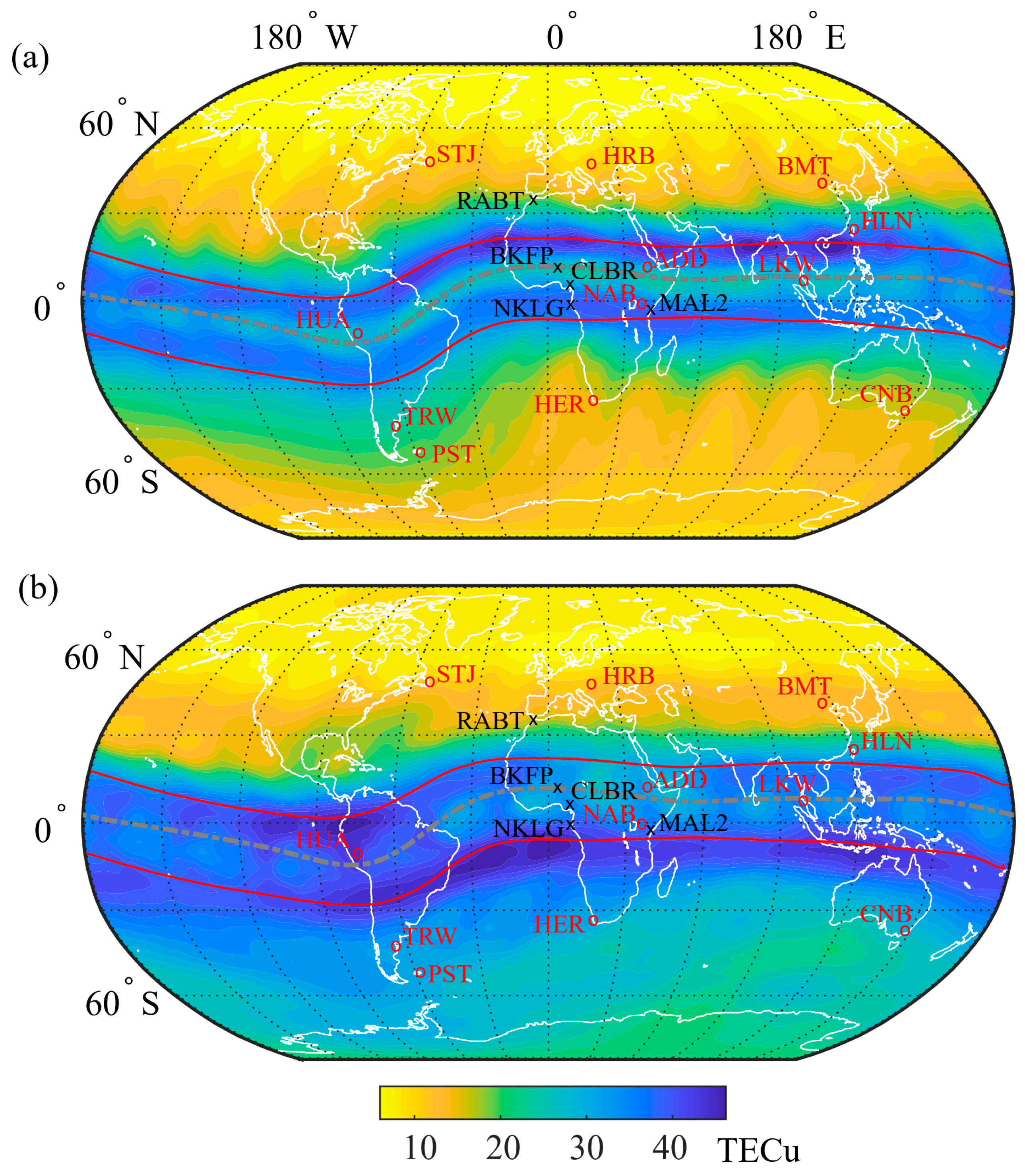
Figure 1. Solar wind and space weather conditions during the storm of February 2014 from different indices: (a) solar flux, (b) SW plasma temperature, (c) SW proton density and SW plasma pressure, (d) SW plasma beta parameter, (e) SW plasma density ratio between alpha and proton, (f) SW speed, (g) IMF Bz component and total field, (h) merging (Em) and eastward zonal (Ey) electric fields, (i) AE index, and (j) SYM-H and Am index (in red). The SSCs and HSSW are highlighted with vertical yellow and green lines, respectively.
Atmosphere 13 00518 g001
Figure 2. Low latitude TEC variations (a,c,e,g,i). The black lines show TEC median (background); blue bins (b,d,f,h,j) show the relative TEC percentage of disturbance. The SSCs and HSSW are highlighted with vertical yellow and green lines, respectively.
Atmosphere 13 00518 g002
Figure 3. The EEJ variations for (a,b) America, (c,d) Africa, and (e,f) Asia. The median is shown as background EEJ. The disturbance of EEJ (dEEJ) is included for each case in blue color (b,d,f). The SSCs and HSSW are highlighted with vertical yellow and green lines, respectively.
Atmosphere 13 00518 g003
Figure 4. The PPEF variations for (a,b) America, (c,d) Africa, and (e,f) Asia. The median is shown as background PPEF. The disturbance of PPEF (dPPEF) is included for each case in blue color. The SSCs and HSSW are highlighted with vertical yellow and green lines, respectively.
Atmosphere 13 00518 g004
Figure 5. Distribution of median average (a) IRI-2012 TEC and (b) IGS GNSS GIMs TEC during February 2014. Gray dashed line marks the geomagnetic dip equator. Red solid lines mark the profiles used to extract TEC near the EIA crests (approximately ±15° to geomagnetic equator). The coordinates of the GNSS (marked with “x”) and geomagnetic (marked with “o”) stations are listed in Table 1, Table 2 and Table 3.
Atmosphere 13 00518 g005
Figure 6. Low latitude GIMs TEC differences between the IGS products and the PCA-based model set for quiet conditions (Am = 6). The differences are along the (a) southern and (b) northern EIA crests (±15°) and along (c) the magnetic equator, from 10 to 28 February 2014. The profiles used to extract TEC are shown in Figure 5a. The bottom panel (d) shows the mean values along the (ac) profiles. The SSCs and the HSSW are highlighted with vertical yellow and green lines, respectively.
Atmosphere 13 00518 g006
Figure 7. Low latitude GIMs TEC differences between the IRI-2012 model and the PCA-based model set for quiet conditions (Am = 6). The differences are along the (a) southern and (b) northern EIA crests (±15°) and along (c) the magnetic equator, from 10 to 28 February 2014. The profiles used to extract TEC are shown in Figure 5b. The bottom panel (d) shows the mean values along the (ac) profiles. The SSCs and HSSW are highlighted with vertical yellow and green lines, respectively.
Atmosphere 13 00518 g007
Figure 8. Upper atmosphere variability during the February 2014 storm at the African region. From top to bottom, (a) the merging electric field Em, (b) the dPPEF at Africa, (c) SYM-H, Am, Dst indices, (d) the dEEJ at Africa, (ei) the TEC variations measured by GNSS stations in Figure 2, and (h) the GIMs TEC differences between the IGS products and the PCA-based model set for quiet conditions (Am = 6) at the EIA crests and at the magnetic equator (from Figure 5a). The (ei) GNSS stations are classified in terms of the proximity to the (j) EIA crests and magnetic equator profiles. The SSCs and HSSW are highlighted with vertical yellow and green lines, respectively.
Atmosphere 13 00518 g008
Figure 9. Space weather indices: (a) Dst and SYM-H, (b) ASY-D, ASY-H, Am, (ce) Earth’s CI, (f) GEC from IRI-2012 and from UPCG, and (g) GIMs TEC differences between the IGS products and the PCA-based model set for quiet conditions (Am = 6) at the EIA crests and at the magnetic equator (from Figure 5a). The SSCs and HSSW are highlighted with vertical yellow and green lines, respectively.
Atmosphere 13 00518 g009
Table 1. Coordinates and details of the GNSS stations.
CodeNameCountryLatitude (°)Longitude (°)MLat (°)
NKLGN’KoltangGabon0.359.67−8.04
MAL2MalindiKenya−2.9940.19−12.42
CLBRCalabarNigeria4.958.35−4.29
RABTRabatMorocco33.99353.1423.88
BKFPKebbiNigeria12.464.220.63
Table 2. Geomagnetic observatories for EEJ estimation.
CodeNameCountryLatitude (°)Longitude (°)MLat (°)
HUAHuancayoPeru−12.07−75.22−1.80
TRWTrelewArgentina−43.25−65.30−33.05
AEEAddis AbabaEthiopia9.0438.770.18
NABNairobiKenya−1.1636.48−10.65
LKWLangkawiMalaysia6.3099.78−2.32
HLNHualienTaiwan23.912116.86
Table 3. Geomagnetic observatories for CI calculation.
CodeNameCountryLatitude (°)Longitude (°)MLat (°)
STJSt JohnCanada47.60−52.6853.59
PSTPort StanlyFalkland Islands −51.70−57.89−38.12
HRBHurbanovoSlovakia47.8718.19−43.02
HERHermanusSouth Africa −34.4319.23−41.90
BMTBeijing Ming TombsChina 40.3116.234.16
CNBCanberraAustralia −35.32149.36−45.24
Publisher’s Note: MDPI stays neutral with regard to jurisdictional claims in published maps and institutional affiliations.

