A Novel Reference-Based and Gradient-Guided Deep Learning Model for Daily Precipitation Downscaling

Abstract

The spatial resolution of precipitation predicted by general circulation models is too coarse to meet current research and operational needs. Downscaling is one way to provide finer resolution data at local scales. The single-image super-resolution method in the computer vision field has made great strides lately and has been applied in various fields. In this article, we propose a novel reference-based and gradient-guided deep learning model (RBGGM) to downscale daily precipitation considering the discontinuity of precipitation and ill-posed nature of downscaling. Global Precipitation Measurement Mission (GPM) precipitation data, variables in ERA5 re-analysis data, and topographic data are selected to perform the downscaling, and a residual dense attention block is constructed to extract features of them. By exploring the discontinuous feature of precipitation, we introduce gradient feature to reconstruct precipitation distribution. We also extract the feature of high-resolution monthly precipitation as a reference feature to resolve the ill-posed nature of downscaling. Extensive experimental results on benchmark data sets demonstrate that our proposed model performs better than other baseline methods. Furthermore, we construct a daily precipitation downscaling data set based on GPM precipitation data, ERA5 re-analysis data and topographic data.

1. Introduction

Precipitation is a weather phenomenon that affects human activities, and has a profound impact on many climate events [1,2]. It is also an important meteorological element in climate research [3]. Precipitation on climatic time scale can be predicted by general circulation models (GCMs) [4]. However, GCMs require substantial computational resources, such that resolution will inevitably be sacrificed. The current spatial resolution of the GCMs’ output is low, which means that it is difficult to conduct detailed local precipitation of high spatial resolution.

In order to address the above problems, the study of downscaling methods has become a hot topic in meteorology. The purpose of downscaling is to convert the large-scale, low-resolution output of GCMs into more detailed regional climate information. At present, classic downscaling methods include dynamic downscaling and statistical downscaling. The dynamic downscaling method nests low-resolution GCMs into high-resolution regional climate models (RCMs), and uses the GCMs to provide initial and boundary value conditions for RCMs in order to obtain high-resolution prediction information describing regional climate characteristics. Dynamic downscaling resolves better physical processes in regional-, meso-, and local-scale circulation effects, and can be used anywhere [5]. However, it requires substantial computing resources, and is greatly affected by the boundary conditions from GCMs. Statistical downscaling is a data-driven downscaling method that uses years of observational data to establish statistical relationships between large-scale climate conditions and regional climate elements. After the statistical relationship is established, independent observational data are used to test this relationship, which will finally be applied to the large-scale climate information output by the GCM to predict the climate change trends of regional elements. Statistical downscaling methods require a large amount of observational data as a statistical basis and cannot be used in areas where large-scale climate elements are poorly correlated with regional climate elements. As the above two methods have shortcomings, many other methods have been proposed, such as downscaling methods combining statistical and dynamic approaches, as well as machine-learning downscaling methods.

With the advent of the era of big data and the development of computer technology, artificial intelligence has received widespread attention. As a branch of machine learning, deep learning is in the forefront of artificial intelligence. It consists of algorithms that attempt to take advantage of high-level abstraction of data using multiple processing layers consisting of complex structures or multiple non-linear transforms, with the aim of getting closer to its primary goal—artificial intelligence [6]. Deep learning approaches have made great achievements in the fields of natural language processing, computer vision, data mining, etc. In recent years, deep learning has been gradually applied to many other fields, and some successful practices have also been obtained. Weather forecasting requires a numerical forecast model to simulate weather changes with respect to initial data, which needs a large number of equations to be calculated. A recurrent neural network has been successfully applied to near-weather forecasting, and has achieved good results. As for downscaling, we can also attempt to find suitable methods in deep learning and integrate them into meteorological downscaling. As a branch of computer vision, single-image super-resolution (SISR) aims to use deep-learning methods to generate high-definition pictures with blurred pictures as input [7], which is quite similar to climate downscaling to a certain extent. Although both use low-resolution data as input to obtain high-resolution data, there is a great difference between them. The typical input in SISR is images, which consist of three channels. The input of climate downscaling is usually observed or simulated climate data, and the output is a certain meteorological element with only a single channel. At the same time, as a meteorological feature, meteorological elements have many spatial characteristics, dynamic characteristics related to physical laws, and a certain meteorological element related to many other meteorological elements, all of which restrict the downscaling process. Therefore, integrating SISR into meteorological downscaling poses a challenge.

Many methods have been used to downscale precipitation to meet the needs of climate research and operational application. Wang et al. used a nonlinear regression model and introduced longitude and latitude based on processed normalized difference vegetation index and a digital elevation model to stimulate precipitation in the Qilian Mountains [8]. Many machine-learning methods are also used for precipitation downscaling. Elnashar et al. used a gradient-boosting regressor, support vector regressor, and artificial neural network to downscale the Tropical Rainfall Measuring Mission (TRMM) precipitation products to 1 km, and found that the artificial neural network yielded the best performance when simulating the annual TRMM precipitation [9]. A downscaling–merging scheme based on random forest and cokriging was presented for acquiring high-precision and high-resolution precipitation data by Yan et al [10]. Based on wide coverage and high temporal and spatial resolution of remote sensing data, many methods have been applied to precipitation downscaling, but few people have applied SISR to precipitation downscaling using remote sensing data.

In this paper, we propose a novel reference-based and gradient-guided deep learning model (RBGGM). The model is divided into three branches: A precipitation branch, a gradient branch, and a reference branch. The precipitation branch uses residual dense channel attention block as the main structure, and low-resolution (LR) precipitation and multiple meteorological element fields as the input. In order to make full use of the discontinuous feature of precipitation, the gradient field is introduced and then reconstructed in gradient branch. At the same time, as the object of downscaling is to find a suitable solution in high-resolution (HR) space, the space of the possible functions that map LR to HR precipitation is extremely large, which leads to an ill-posed problem in the task [11]. We extracted the features of high-resolution monthly precipitation as a reference to resolve the ill-posed nature of downscaling in the reference branch. Finally, the gradient feature, along with the reference feature, are utilized in the precipitation reconstruction in order to guide the precipitation downscaling process, such that the reconstruction result avoids over-smoothing in the spatial distribution and ensures appropriate spatial characteristics. Our contributions can be summarized as follows:

• For the task of downscaling of daily precipitation data, we selected daily average values for multiple meteorological elements. By correcting and filtering the data, a meteorological data set suitable for daily precipitation downscaling tasks was constructed.
• In order to extract the characteristics of different meteorological elements, we constructed a feature-extraction module called the residual dense channel attention block (RDCAB). The RDCAB has a strong convergence ability and great recognition ability for different features, both of which are suitable for the considered task.
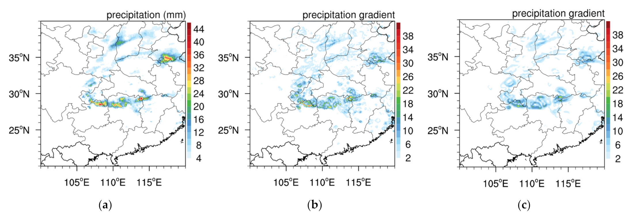
• We also explored the effects of using the gradient feature and reference feature on precipitation downscaling. Due to the spatial discontinuity of precipitation itself, the precipitation area often corresponds to the area of a large precipitation gradient, such that its gradient information is also of great significance for precipitation reconstruction. Due to the ill-posed nature of precipitation, we used reference feature of high-resolution monthly precipitation data as a supplement based on deformable convolution.
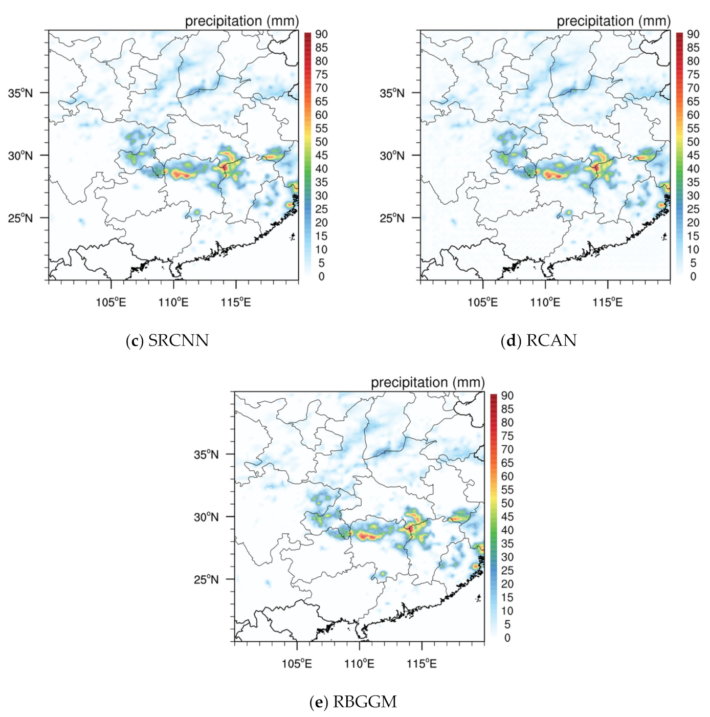
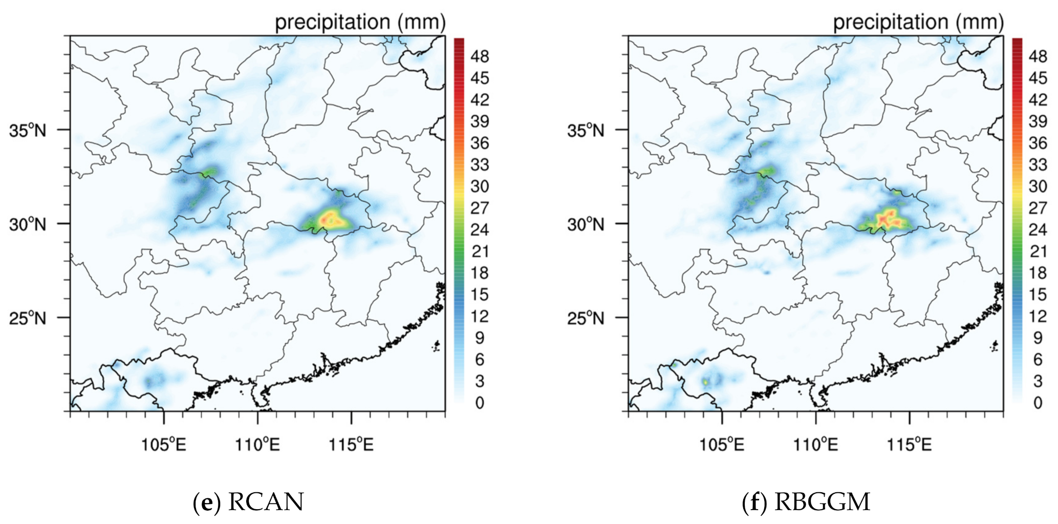
• We propose a precipitation-downscaling model, named gradient-guided deep learning model (RBGGM), which is divided into a precipitation branch, a gradient branch, and a reference branch. The precipitation branch completes the downscaling of precipitation, while the gradient branch and the reference branch guide the downscaling of precipitation. Experiments show that our approach restores more details in areas with heavy precipitation.

2. Related Work

2.1. Single-Image Super-Resolution

In recent years, many achievements have been achieved in the field of single-image super-resolution (SISR). First, super-resolution convolutional neural network (SRCNN) was proposed, which uses three convolutional layers for feature extraction, feature non-linear mapping, and final reconstruction [12]. The up-sampling operation appeared afterwards. Fast super-resolution convolutional neural network (FSRCNN) performs deconvolution for up-sampling, and efficient sub-pixel convolutional neural network (ESPCN) contains a sub-pixel convolution layer for up-sampling [13,14]. Very deep convolutional network (VDSR) has a deeper number of layers, and introduces a global residual structure [15]. Deep recursive residual network (DRRN) introduces a chained local residual structure combined with a global residual structure and further deepens the number of network layers, thus strengthening the convergence ability of the network [16]. Subsequently, the network structure has been improved substantially. Lai et al. proposed the Laplacian pyramid super-resolution network (LapSRN) to progressively reconstruct the sub-band residuals of high-resolution images and changed the L2-type loss function to L1-type, to achieve better results [17]. A generative adversarial network has also been used for super-resolution reconstruction, which uses a perceptual loss function and a two-branch network to make the reconstructed texture clearer [18]. Residual channel attention network (RCAN) applies a channel attention mechanism to the residual block and uses global average pooling to distribute the weights of the channels in the residual block, which effectively strengthens its feature-extraction ability [19]. Ma et al. introduces a structure-preserving super-resolution method (SPSR) to alleviate undesired structural distortions while maintaining the generative adversarial network (GAN) structure in order to generate perceptually pleasant details [20].

2.2. Reference-Based Super-Resolution

Due to the ill-posed nature of SISR, most of the existing methods suffer from blurring when they need to restore the fine details lost in the low-resolution image. Reference-based super-resolution (RefSR) uses rich textures from HR reference images to compensate for missing details in the low-resolution image, alleviates the ill-posed problem, and generates more detailed and realistic textures with the help of reference images. Recent RefSR methods can be roughly divided into two categories: patch matching and image alignment. Some studies have used patch matching to find similar features in reference images and apply them to low-resolution images. Zhang et al. drew on the idea of Neural Texture Transfer in image stylization and used the textures in reference images to compensate for detailed information loss in the low-resolution image [21]. The advantage of patch matching is that it can match long-distance dependencies, but patch-based synthesis is inherently incapable of handling the non-rigid image deformation caused by viewpoint changes and causes grid artifacts. RefSR network using cross-scale warping (CrossNet) uses an encoder to extract the spatial features of a reference image and the low-resolution image, and uses a decoder to merge these feature images and generate an HR image [22].

2.3. SISR for Precipitation Downscaling

Some scholars have now introduced SISR into the work of precipitation downscaling. Originally, SRCNN is used in precipitation downscaling, and stacked SRCNN is used to boost the resolution of the higher factor [23,24]. And then U-net networks, deep residual network (DRN), and convolutional neural network (CNN) are also used in precipitation downscaling [25,26,27]. However, the above work only ensures the migration of the network, without the modification of the network. Mu et al. considered the multiscale spatial correlations and chaos in multiple climate events, and built up a two-stage deep learning model [28]. Cheng et al. enhanced the effect of precipitation downscaling by improving the residual structure in LapSRN to a residual dense structure [29]. However, the nature of precipitation and downscaling itself is not further considered: (1) The spatial distribution of precipitation is discontinuous, so the spatial abruptness is very important, and the traditional model will produce a smoothing effect, resulting in great deviations in the spatial distribution; (2) Downscaling is ill-posed, and how to solve the ill-posed nature of downscaling to obtain better downscaling results is particularly important. Therefore, based on the above discussion, we construct a deep learning network suitable for precipitation downscaling.

3. Dataset

3.1. Study Area

Figure 1 shows the study area, which spans from 20° N to 40° N and from 100° E to 120° E. It mainly covers Central China, East China, and South China. Since the study area is located in the East Asian monsoon climate zone, the spatial distribution and seasonal distribution of precipitation are extremely uneven, resulting in frequent droughts and floods. Therefore, the study of this area is highly representative. The basic information of the used data sets is summarized in

Table 1. Summary of the data sets used in this study.

Data Set	Resolution	Frequency	Variable	Period	Producer
GPM_3IMERGDF	0.1°	1 day	Daily precipitation	2000–present	NASA GSFC PPS
GPM_3IMERGM	0.1°	1 month	Monthly precipitation	2000–present	NASA GSFC PPS
ERA5 Re-analysis Data	0.25°	1 h	Temperature, relative humidity, etc.	1979–present	ECMWF
DEM	0.25°	/	height	/	ALOS

.

3.2. GPM Precipitation Data

The GPM (global precipitation measurement mission) is a new generation of global precipitation measurement remote sensing satellite projects, based on the Tropical Rainfall Measuring Mission (TRMM) [30]. GPM data products can be mainly divided into three types: Level-1, Level-2, and Level-3. Level-1 is the data directly received by the detection instrument, Level-2 is the geophysical variable data derived based on Level-1, and the data in Level-3 is interpolated to grid points with fixed time and spatial resolution based on Level-2. The spatial resolution of GPM level-3 data is 0.1°, which is higher than that of the TRMM 3B42 data. It also covers the world and has a temporal resolution of 0.5 h, which significantly improves the spatial coverage and the temporal resolution [31]. We selected GPM IMERG Final Precipitation L3 1 month 0.1° × 0.1° V06 (GPM_3IMERGM) and GPM IMERG Final Precipitation L3 1 day 0.1° × 0.1° V06 (GPM_3IMERGDF) from 1 June 2000 to 31 December 2019. The variables we used are HQprecipitation.

3.3. ERA5 Re-Analysis Data

The ERA5 re-analysis data are released by the European Meteorological Center, which regularly uses predictive models and data assimilation systems to re-analyze archived observations, thereby creating a data set describing the atmosphere, land, and ocean since the 1970s [32]. The ERA5 re-analysis data contain more than 20 physical quantities, including atmospheric physical quantities such as temperature, pressure, humidity, and wind. Atmospheric temperature, humidity, and other atmospheric physical quantities have an important influence on precipitation, so we used hourly data of temperature and relative humidity on $850 \mathrm{hpa}$. The data were in the same time range as GPM precipitation data.

3.4. Topography

The terrain can block the flow of air and lift it, and hence has an important impact on precipitation; for example, more precipitation is typically observed on a windward slope than on a leeward slope. Therefore, we also used ground elevation data, taking into account the influence of terrain on precipitation. We used the digital elevation model (DEM) of the Japan ALOS satellite.

3.5. Data Pre-Processing

The daily precipitation data of GPM are two-dimensional grid data with format $\left[\mathit{lon},\mathit{lat}\right]$, which we transposed to $\left[\mathit{lat},\mathit{lon}\right]$. The original precipitation was coarsened to create a low-resolution data set at 0.25° through spatial interpolation, which served as the input. The format of the ERA5 re-analysis data is $\left[\mathit{time},\mathit{level},\mathit{lat},\mathit{lon}\right]$. When a single time is selected, the meteorological element fields all day long cannot be reflected, and the response to daily precipitation is incomplete; on the other hand, when multiple times are selected, too many inputs cause the model to become too bloated. Therefore, we selected the daily average type; that is, we averaged the ERA5 re-analysis data in the first dimension. We also selected the geopotential height of $850 \mathrm{hpa}$ in the second dimension, as the data at this height have a significant impact on precipitation. Finally, after averaging the time dimension and selecting $850 \mathrm{hpa}$ levels, each meteorological element was a two-dimensional matrix $\left[\mathit{lat},\mathit{lon}\right]$, consistent with precipitation data.

It has been experimentally found that if the input of the model is only low-resolution precipitation data, the training results are not satisfactory and the downscaled output obtained cannot simulate the characteristics of precipitation well. This may be because if the input data are too monotonous, the model cannot extract more features, thus resulting in poor results. At the same time, precipitation is a non-continuous, extremely unevenly distributed meteorological element field that is prone to large areas of null values, which leads to great difficulties in the training of the model. Therefore, we used temperature and relative humidity in the ERA5 re-analysis data and DEM to increase the diversity of the data and provide more features for the model.

In order to fuse low-resolution precipitation, temperature, humidity, and DEM data, we used a multi-channel fusion scheme. First, we added one dimension to all two-dimensional data, such that they became $\left[1,\mathit{lat},\mathit{lon}\right]$. Then, we concatenated the four kinds of data in the first dimension to yield $\left[\mathit{pattern},\mathit{lat},\mathit{lon}\right]$, where the first dimension represents the data type (see Figure 1). Due to the different distributions of the various meteorological elements, in order to prevent over-fitting during the training process, and to appropriately learn the characteristics of each physical quantity, we normalized all of the data. Common normalization schemes include max–min normalization and Z-score normalization. As the precipitation data were all non-negative, and there was a wide range of 0 value distribution, we chose max–min normalization. Therefore, our input data were all distributed in the range (0, 1)

Due to the low probability of precipitation events occurring in the weather, there were many samples with no or sporadic precipitation in the data set. Sporadic precipitation samples indicate that grid points with precipitation (value greater than 0.1mm) account for less than 1% of the total grid points. The training set is important for deep learning, so we eliminated no-precipitation or sporadic-precipitation samples and only retained more than 4000 samples. In the experiments, the data set was divided into three parts: a training set, a validation set, and a test set (with a ratio of 8:1:1). Finally, we obtained a downscaled data set based on re-analysis, precipitation, and topographic data.

4. Methods

In this section, we introduce (1) feature extraction module, (2) gradient feature for precipitation downscaling, (3) reference feature extraction of monthly precipitation, (4) reference-based and gradient-guided model (RBGGM) for precipitation downscaling, and (5) loss functions, among others.

4.1. Feature Extraction Module

4.1.1. Channel Attention Block

In order to enable the network to obtain more information for downscaling, we added a variety of data, such as temperature, relative humidity, and topography, into the input; however, these data play different roles in establishing the output precipitation. In order to ensure that the network better extracts features from the input, we introduced a channel attention block (see Figure 2). Many different kinds of channel attention modules have been proposed. The traditional Squeeze-and-Excitation Module (SEM) (see Figure 2a) uses the global characteristics of each channel to represent the importance of each channel, but ignores spatial information [33]. As the spatial distribution of precipitation is extremely uneven, the average pooling operation is not suitable for the special characteristics of precipitation. Therefore, we discarded SEM and chose a new attention module, called the Self Channel Attention Module (SCAM) (see Figure 2b) [34]. Based on self-attention mechanism, it uses channel matrix operation to capture the channel dependence between any two channel maps, and uses the weights of the channel attention matrix to update each channel map.

4.1.2. Residual Dense Channel Attention Block

We constructed the Residual Dense Channel Attention Block (RDCAB) to increase the feature extraction capability of the model. In order to increase the learning ability, the network can be gradually deepened; however, this may cause the gradient to disappear or explode, which will affect the effectiveness of the network to a certain extent. We used the idea of residual dense block to increase the convergence speed of the network and make the network perform better (see Figure 3) [35]. At the same time, the attention module can extract channel information and increase the model’s discrimination ability. Therefore, SCAM was added to the residual dense block to obtain RDCAB (see Figure 4). The formula is as follows:

$$F_i=F_{i-1}+R_i\left(F_{i-1}{}^{\prime }\right),$$

(1)

where $R_i(\cdot )$ denotes the function of the SCAM, $F_{i-1}$ and $F_i$ are the input and output of the RDCAB, respectively, and $F_{i-1}{}^{\prime }$ is the feature of $F_{i-1}$, which is completed by a dense block (RB):

$$F_{i-1}{}^{\prime }=D_i\left(F_{i-1}\right),$$

(2)

where $D_i\left(\cdot \right)$ denotes the operation of the dense block (see Figure 3). RB uses a feed-forward method to connect each layer to all other layers. We found that, compared to the residual group used in [19], RDCAB strengthens the feature propagation, thus increasing the convergence speed while also greatly reducing the number of parameters.

4.2. Gradient Feature for Precipitation Downscaling

Meteorological elements such as temperature, humidity, and air pressure are continuous quantities, and the changes in the atmosphere are continuous, while precipitation is a discontinuous meteorological element with an extremely uneven spatial distribution and large changes in intensity. Therefore, downscaling precipitation is more difficult than downscaling other elements. Figure 5 shows the original precipitation distribution, the corresponding gradient map, and the gradient map corresponding to the interpolation method on 5 September 2014. It can be seen that the precipitation area corresponds to the gradient area in the gradient map, and the large precipitation area also corresponds to a large gradient area; thus, gradient feature is important.

Although the traditional interpolation method can reconstruct the distribution of precipitation, it excessively smooths the precipitation distribution, that is, the gradient value is smaller, which will destroy the sudden changes in precipitation. This indicates that in order to further improve the downscaling effect, it is important to restore the uneven spatial distribution of precipitation. For this reason, in this article, in addition to the spatial downscaling of the original precipitation data, we also downscale the first derivative distribution of the precipitation data as a guide. In this way, the spatial discontinuity characteristics of precipitation are fully restored.

4.3. Reference Feature Extraction of Monthly Precipitation

Based on the RefSR method, we used high-resolution monthly precipitation data to compensate for the ill-posed nature of precipitation downscaling based on deformable convolution (see Figure 6). Learning mapping from LR to HR precipitation is typically an ill-posed problem since there exist infinitely many HR precipitations that can be upscaled to obtain the same LR precipitation [36]. Therefore, the features in high-resolution monthly precipitation data are used to help find a more suitable HR precipitation for our task of downscaling. In order to find features related to daily precipitation, we used deformable convolution [37]. Deformable convolution obtains the desired features by generating offsets for convolution kernels. First, we used the features and their gradients of monthly precipitation and the generated precipitation to construct a reference feature map and a generated feature map, respectively. We then looked for correlations between the reference feature map and the generated feature map, which rely on the offset generated by the convolution. Finally, we applied the offset to the reference feature map in order to obtain the output feature map, and put it into the fusion module through a convolutional layer.

4.4. RBGGM for Precipitation Downscaling

As shown in Figure 7, we constructed our proposed Reference-based and Gradient-guided Model (RBGGM) in three parts: A precipitation branch, a gradient branch, and a reference branch.

The precipitation reconstruction part includes a shallow extraction module, a deep residual extraction module, and an up-sampling module. We used low-resolution precipitation, temperature, humidity, and DEM data as the input $I_{LR}$, and high-resolution precipitation as the output $I_{SR}$. As investigated in a previous SISR model [38], we used only one convolutional layer to extract the shallow feature $F_{DF1}{}^P$ from the input:

$$F_{DF1}{}^P=H_{CON}(I_{LR}),$$

(3)

where $H_{CON}(\cdot )$ denotes the convolution operation. After shallow feature extraction, $F_{DF1}{}^P$ was then used for deep residual extraction with several RDCABs:

$$F_{DF2}{}^P=H_{DF}\left(F_{DF1}{}^P\right),$$

(4)

where $H_{DF}(\cdot )$ denotes the deep residual extraction operation, which contains several RDCABs. Part of the intermediate features were retained and used as the input for the gradient module. At the same time, a long skip connection was introduced to stabilize the training of the network. $F_{DF2}{}^P$ is the output feature, which was used as the input for the up-sampling module:

$$H_{UP}{}^P=H_{UP}(F_{DF2}{}^P),$$

(5)

where $H_{UP}(\cdot )$ denotes an up-sampling module. Up-sampling can be carried out through interpolation, deconvolution, and sub-pixel convolution. Interpolation is the simplest method, and its parameters cannot be optimized through training. Deconvolution can be optimized through training, but it is prone to the checkerboard effect, so we chose sub-pixel convolution. The process of sub-pixel convolution is as follows: First, the input $w\ast h\ast 1$ generates the feature map $w\ast h\ast c^2$ through convolution, and the feature map is then converted to the result $\left(w\ast c\right)\ast \left(h\ast c\right)$ in order to achieve up-sampling. The up-sampling result is spliced with the gradient branch feature and then input into the fusion module:

$$H_{\mathit{OUT}}{}^P=H_{\mathit{CON}}\left(H_{\mathit{UP}}{}^P,H_{\mathit{UP}}{}^G,H_{\mathrm{Ref}}\right),$$

(6)

where $H_{\mathit{UP}}{}^P$ is the precipitation reconstruction feature, $H_{\mathit{UP}}{}^G$ is the precipitation gradient feature, and $H_{\mathrm{Ref}}$ is the reference feature of monthly high-resolution precipitation. $H_{\mathit{CON}}(\cdot )$ is the fusion process, which indicates that the three types of features are fused to obtain the final precipitation distribution. Here, we use RDCAB as the fusion module, as the RDCAB module can fully extract the features. Finally, $H_{\mathit{OUT}}{}^P$ goes through the reconstruction module to obtain the precipitation output:

$$I^{\mathit{SR}}=H_{\mathit{REC}}(H_{\mathit{OUT}}{}^P),$$

(7)

where $H_{\mathit{REC}}(\cdot )$ is the reconstruction module, which is composed of a convolution operation and a rectified linear unit (ReLU) activation function, and $I^{\mathit{SR}}$ is the final high-resolution precipitation output.

The gradient branch was used to reconstruct the precipitation gradient information, in order to ensure the spatial discontinuity of precipitation. Similar to the precipitation reconstruction branch, the main structure is divided into a feature extraction module and an up-sampling module. The difference from the precipitation module is that, during the reconstruction process, we used the precipitation feature, which can aid in the reconstruction of gradient information and reduce the complexity of the model. We chose the RDCAB as the gradient extraction module and sub-pixel convolution as the up-sampling module.

For the goal of precipitation downscaling, we selected the gradient of precipitation, $P_{\mathit{LR}}$, as the input. We obtained the gradient of the input through the gradient module:

$$F_0{}^G=M\left(P_{\mathit{LR}}\right),$$

(8)

where $M(\cdot )$ represents the process of obtaining the gradient. We used the difference between two adjacent grid points to represent the gradient, based on differentiation instead of differencing:

$$\begin{array}{l}{I}_x\left(x,y\right)=I\left(x+1,y\right)-I\left(x-1,y\right)\\ I_y\left(x,y\right)=I\left(x,y+1\right)-I\left(x,y-1\right)\\ \nabla I\left(x,y\right)=\left(I_x\left(x,y\right),I_y\left(x,y\right)\right)\\ M\left(I\right)={‖\nabla I‖}_2\end{array}$$

(9)

where $M\left(\cdot \right)$ denotes the gradient operation. We did not use the vector form field to represent the gradient field as the scalar field is enough to describe the precipitation gradient. We then used multiple RDCABs for feature extraction:

$$F_{\mathit{DF}1}{}^G=H_{\mathit{RG}}(F_0{}^G),$$

(10)

where $H_{\mathit{RG}}$$(\cdot )$ denotes the feature extraction structure, which contains multiple blocks, each of which consists of a convolutional layer and an RDCAB. Before each one, the intermediate output of the precipitation reconstruction branch was introduced to enhance the reconstruction of the precipitation gradient. The output, $F_{\mathit{UP}}{}^G$, was then introduced to the up-sampling module:

$$F_{\mathit{UP}}{}^G=H_{\mathit{UP}}(F_{\mathit{DF}}{}^G)$$

(11)

where $H_{\mathit{UP}}(\cdot )$ is achieved by sub-pixel convolution. The output, $F_{\mathit{UP}}{}^G$, is divided into two branches: one branch flows to the fusion module to guide the reconstruction of precipitation, and the other flows to the convolutional layer to restore the high-resolution gradient.

The reference branch is used to extract feature maps related to precipitation downscaling in high-resolution monthly precipitation using deformable convolution:

$$H_{\mathrm{Ref}}=H_{\mathit{Def}}\left(P_{\mathit{Mon}},M\left(P_{\mathit{Mon}}\right)\right),$$

(12)

where $H_{\mathit{Def}}\left(\cdot \right)$ denotes the deformable convolution operation, and $M\left(\cdot \right)$ denotes the gradient operation. The output flows to the fusion module after the convolutional operation, supplementing the precipitation reconstruction.

4.5. Loss Functions

We chose the L1 loss function as the main function to calculate the error between the generated and the original precipitation. Secondly, based on the discontinuous feature of precipitation, we constructed a gradient loss function, which is conducive to the reconstruction of the precipitation distribution. We used the gradient operation to obtain the gradients of the original precipitation and the generated precipitation, and then calculated the error through the L1 loss function.

The output of the precipitation branch is the precipitation reconstruction result, $I^{\mathit{SR}}$, while the corresponding high-resolution precipitation is $I^{\mathit{HR}}$. We used the L1 and gradient loss functions to calculate the error between the generated precipitation and the original precipitation:

$$L^P=L_1\left(I^{\mathit{SR}},I^{\mathit{HR}}\right)+L_1\left(M\left(I^{\mathit{SR}}\right),M\left(I^{\mathit{HR}}\right)\right),$$

(13)

where $L_1\left(\cdot \right)$ denotes the L1 loss function and $M\left(\cdot \right)$ denotes the gradient operation.

We also used the L1 loss function to calculate the error between the generated gradient $G^{\mathit{SR}}$ and the original gradient $G^{\mathit{HR}}$ in the gradient reconstruction, such that the final loss function of the model consisted of two parts:

$$L=\alpha L^P+\beta L_1\left(G^{\mathit{SR}},G^{\mathit{HR}}\right)\mathbf{,}$$

(14)

where $L_1\left(\cdot \right)$ denotes the L1 loss function, $L^P$ denotes the loss function of the precipitation branch, and $\alpha$ and $\beta$ are trade-off parameters for the different losses. We set $\alpha$ to 5 and $\beta$ to 1.

4.6. Baseline Methods

We compared RBGGM against a few commonly used downscaling baselines: bi-linear interpolation, SRCNN, and RCAN. SRCNN is a classic downscaling method with three-layer convolution for feature extraction, non-linear feature mapping, and final reconstruction [11]. RCAN is a deep residual channel attention network that contains a residual structure composed of residual attention blocks [19].

4.7. Evaluation Metrics

In meteorology, the evaluation of precipitation accuracy is generally based on binarization. The prediction and the reality are divided into 0 or 1 by a threshold, where 1 means greater than the threshold, and 0 means less than the threshold. Relevant indicators include the critical success index (CSI), false alarm rate (FAR), and probability of detection (POD) [39]:

$$\begin{array}{c}\mathit{CSI}=\frac{\mathit{hits}}{\mathit{hits}+\mathit{false} \mathit{alarms}+\mathit{misses}},\\ \mathit{POD}=\frac{\mathit{hits}}{\mathit{hits}+\mathit{misses}},\\ \mathit{FAR}=\frac{\mathit{false} \mathit{alarms}}{\mathit{hits}+\mathit{false} \mathit{alarms}}.\end{array}$$

(15)

As shown in

Table 2. Precipitation test indicators.

Confusion Matrix		Prediction
		1	0
Reality	1	hit	miss
	0	false alarm	correct negative

, a hit represents the total number of stations where the prediction is the same as the real precipitation status. A false alarm indicates the number of stations where the prediction does not match reality. A miss represents the number of stations where real precipitation occurs but is not predicted. We set the threshold to 0.1, as this is the critical value for the presence of precipitation. These indicators are not sufficient for an accurate evaluation, as when small changes occur during downscaling, the data around the threshold can easily be divided into another area. Therefore, we used the mean absolute error (MAE) and correlation coefficient (CC), as well as their probability distribution functions, as supplements.

5. Results

We trained RBGGM and the baseline models on the constructed data set. We chose the Adam optimizer, and the initial learning rate was set to 0.0001. At the same time, we adopted an exponential learning rate decay strategy to improve the stability of training, and set gamma to 0.95. The sample size was set to 16. All models were based on Pytorch. We trained all models on two NVIDIA GeForce RTX 3090 units, and each model was trained for about 100 epochs.

We compared the performance of different methods through the indicators and precipitation distributions. We also conducted extensive experiments using TRMM precipitation data and ERA5 re-analysis precipitation data. Finally, we attempted the downscaling process with different multiples.

5.1. Performance of the Generated Precipitation

We trained SRCNN, RCAN, and RBGGM on the training set, then calculated the relevant evaluation indicators on the test set. Bi-linear method directly verified the effect on the test set.

5.1.1. Performance on Evaluation Indicators

For each method, we conducted a comparative experiment on the test set. We calculated the CSI, POD, FAR, mean absolute error (MAE), and correlation coefficient (CC) indicators. The results are shown in

Table 3. Quantitative evaluation of different methods.

Algorithm	MAE	CC	CSI	POD	FAR
Bi-linear	0.301	0.950	0.826	0.856	0.041
SRCNN	0.294	0.952	0.802	0.845	0.060
RCAN	0.278	0.954	0.841	0.916	0.089
RBGGM	0.263	0.962	0.848	0.923	0.086

.

As shown in Table 3, for all deep learning models, a lower MAE value and a higher CC value were obtained compared with the interpolation method, which indicates that deep learning methods are effective when applied to precipitation downscaling. Compared with SRCNN, although RCAN and RBGGM lagged behind in terms of POD, they improved the other indicators to varying degrees. This demonstrates that compared with traditional convolution, the residual dense block architecture based on an attention mechanism has a better effect in the feature extraction of meteorological elements. The RBGGM was superior to other methods in terms of many indicators, especially MAE and CC, indicating that the fusion of gradient information and reference-based monthly precipitation has a certain positive effect on precipitation downscaling. We also obtained the probability density functions (PDFs) for MAE and CC, which are plotted in Figure 8. As can be seen, RBGGM had a lower MAE distribution and a higher CC distribution compared to other methods, showing that RBGGM can obtain results closer to the real precipitation field in precipitation downscaling.

5.1.2. Performance on Precipitation Distribution

The texture of the downscaling output is expected to have local-scale variability that reflects the impact of sub-grid processes. Texture evaluation is of importance, as the local-scale variability of precipitation is a key factor for predicting the hydrological response to atmospheric conditions [40]. In order to evaluate the performance of the proposed RBGGM on texture, we obtained the downscaling results of each method separately, based on the test set. Then we analyzed the texture performance through the precipitation downscaling distribution.

We chose the precipitation event as it is representative for analyzing the texture of precipitation distribution. The examples we selected included weather conditions such as squall lines and local convection. These weather conditions can cause heavy precipitation processes [41], and their spatial distribution varies greatly. There was not just one heavy precipitation center in each example, which indicates that there may be multiple weather systems that cause precipitation; thus, it was considered possible to more comprehensively demonstrate the performance of different downscaling methods under multiple precipitation situations.

The precipitation distributions for different methods are shown in Figure 9. All methods obtained a similar precipitation range to real precipitation, but there were differences in the spatial distribution of precipitation. The results of the bi-linear method were the worst in terms of the spatial distribution. The large value area of real precipitation was greatly weakened in the bi-linear results, and many heavy precipitation centers disappeared, leading to the absence of heavy precipitation in actual downscaling applications. For the deep-learning models, the large value area of precipitation can be more completely described, which also indicates that deep-learning methods are more suitable for downscaling work. At the same time, as other precipitation-related data (i.e., temperature, humidity, and topography) were used, more information could be included in the downscaling results. An enlarged map of heavy precipitation distribution is shown in Figure 10. When comparing real precipitation with the results of SRCNN and RCAN models, we found that the large precipitation area in the results was relatively coarse, and the textures of the heavy precipitation area were not well-restored. Due to the high resolution of GPM precipitation, it is difficult to restore the extreme values of precipitation during the downscaling process; however, extreme precipitation events are very important for climate research and analysis [42]. The proposed RBGGM model had a better performance compared with other methods. It could restore more texture features in areas with large precipitation values, demonstrating that our approach can achieve better performance when downscaling torrential rain.

5.2. Scalability on TRMM Data Set and ERA5 Re-Analysis Data Set

There are many different types of precipitation data, such as satellite fusion data, model post-processing data, and re-analysis data. The object of downscaling is usually the output result of the model. Therefore, the precipitation downscaling object cannot be limited to GPM data. We extracted daily precipitation data from TRMM satellite data and ERA5 re-analysis data, and explored the effects of our model on these two types of data. We used the trained model as the test model. The temperature, humidity, and terrain data in the input remained unchanged, while the TRMM satellite precipitation data and re-analysis data precipitation data were used as input to obtain high-resolution precipitation outputs. At the same time, we compared the results of the proposed method with those of bi-linear interpolation, SRCNN, and RCAN.

The results for TRMM precipitation using the four considered methods are shown in Figure 11. The downscaling results of all methods maintained a strong precipitation area, and the precipitation distribution was consistent. However, based on careful observation, the texture characteristics of the precipitation center could not be fully restored by bi-linear interpolation, SRCNN, or RCAN. The distribution of precipitation centers in the results of these methods was too smooth and only had a rough outline. The proposed RBGGM model not only restored the overall precipitation distribution, but also showed the texture distribution of the precipitation center. At the same time, due to the use of reference-based and gradient-guided methods, we could introduce more precipitation feature information to reconstruct better precipitation distribution.

5.3. Precipitation Downscaling Methods for Different Downscaling Factors

According to the demands of different tasks, we may need to use different downscaling schemes for the output of the GCMs. Therefore, in addition to the above-mentioned downscaling factor of 2.5, we also verified model performance when using different downscaling factors in order to further verify the generalization ability of the model. In addition to precipitation, input to the model included temperature, humidity, and topography, which served as additional supplementary information. As these are continuous quantities, in contrast to precipitation, we interpolated them to different resolutions according to the needs of the task. We designed a downscaling model with a downscaling factor of 4 to further verify the effect of the model. We interpolated GPM precipitation ERA5 data and topography to 0.4° as input. We trained the SRCNN, RCAN, and RBGGM models, respectively. Finally, all methods were verified on the test set.

As shown in Figure 12, the 0.4° precipitation input led to loss of most of the heavy precipitation information, and only a small amount of heavy precipitation was retained, which made it difficult to restore the texture characteristics of precipitation when using bi-linear and SRCNN methods. Although the result of RCAN was better, it still did not fully restore the precipitation texture. The result of our proposed RBGGM method was much better as it restored most of the texture characteristics of the precipitation distribution. The PDFs of MAE and CC are also shown in Figure 13. We can see that RCAN does not outperform bi-linear on MAE and CC indices due to the lack of too many precipitation details for low-resolution precipitation input, and SRCNN even performs poorly. Our proposed RBGGM outperforms other methods, especially on CC index, indicating that the downscaling results of RBGGM can obtain more accurate precipitation distribution.

6. Discussion

The data used in this paper are satellite fusion precipitation data, which have high resolution in both time and space. In terms of time, we used 20 years of data for the construction of the data set, such that the model achieved a strong generalization ability. In terms of space, the high resolution of the satellite data posed a great challenge to the performance of the model. The precipitation input precluded some small areas with heavy precipitation from being simulated due to an excessive loss of information. However, better performance of our proposed model indicated that the model is capable of downscaling other climate models.

The proposed model uses not only the gradient guidance method but also the reference-based super-resolution method. Due to the discontinuous distribution of precipitation, the above methods are highly suitable for precipitation reconstruction. The reference-based data we used were monthly precipitation data. We may also utilize other satellite remote sensing data related to daily precipitation, such as the high-quality Climate Data Record (CDR) of global infrared measurements from geostationary satellites [43]. We can also conduct experiments to see which kind of data leads to better results.

The object of this article is precipitation downscaling, but we can also apply the proposed model to downscaling tasks pertaining to other meteorological elements. As meteorological elements such as temperature and humidity are continuous physical quantities, and there are often no zero-value areas, they are easier to downscale compared to precipitation. Therefore, we can apply the model proposed in this article to other meteorological elements, such as temperature.

7. Conclusions

In this article, we proposed a novel deep-learning model named RBGGM for daily precipitation downscaling, which simultaneously considers the discontinuous features of precipitation and addresses the ill-posed nature of downscaling. We added some meteorology fields closely related to precipitation such as temperature, humidity, and topography to complement precipitation downscaling, and constructed a feature extraction module based on a residual dense channel attention block. The RBGGM model is divided into three parts: (1) a gradient branch is introduced to assist in precipitation downscaling by downscaling the precipitation gradient; (2) a reference branch utilizes deformable convolution to extract high-resolution precipitation features as a reference feature to address ill-posed nature of downscaling; (3) a precipitation branch obtains the precipitation downscaling result by extracting input features and fusing the above two branches.

We conducted various experiments, which demonstrated that our method can generate a more detailed and accurate precipitation distribution on specific precipitation events and get higher values of CC and lower values of MAE on the entire test set as compared to other baseline methods. At the same time, it also performs well on other data such as TRMM satellite precipitation and higher downscaling factors. The end-to-end model we proposed here can also be used in the downscaling processes of other meteorological elements such as temperature, so it has wide application prospects.

References

1. Villén-Peréz, S.; Heikkinen, J.; Salemaa, M.; Mäkipää, R. Global warming will affect the maximum potential abundance of boreal plant species. Ecography 2020, 43, 801–811. [Google Scholar] [CrossRef] [Green Version]
2. Aryal, Y.; Zhu, J. Evaluating the performance of regional climate models to simulate the US drought and its connection with El Nino Southern Oscillation. Theor. Appl. Climatol. 2021, 145, 1259–1273. [Google Scholar] [CrossRef]
3. Schiermeier, Q. The real holes in climate science. Nature 2010, 463, 284–287. [Google Scholar] [CrossRef] [PubMed]
4. Taylor, K.E.; Stouffer, R.J.; Meehl, G.A. An overview of CMIP5 and the experiment design. Bull. Am. Meteorol. Soc. 2012, 93, 485–498. [Google Scholar] [CrossRef] [Green Version]
5. Politi, N.; Vlachogiannis, D.; Sfetsos, A.; Nastos, P.T. High-resolution dynamical downscaling of ERA-Interim temperature and precipitation using WRF model for Greece. Clim. Dyn. 2021, 57, 799–825. [Google Scholar] [CrossRef]
6. Dong, S.; Wang, P.; Abbas, K. A survey on deep learning and its applications. Comput. Sci. Rev. 2021, 40, 100379. [Google Scholar] [CrossRef]
7. Dai, T.; Cai, J.; Zhang, Y.; Xia, S.; Zhang, L. Second-order attention network for single image super-resolution. In Proceedings of the IEEE/CVF Conference on Computer Vision and Pattern Recognition CVPR 2019, Long Beach, CA, USA, 16–20 June 2019; pp. 11065–11074. [Google Scholar] [CrossRef]
8. Wang, L.; Chen, R.; Han, C.; Yang, Y.; Liu, J.; Liu, Z.; Wang, X.; Liu, G.; Guo, S. An improved spatial–temporal downscaling method for TRMM precipitation datasets in Alpine regions: A case study in northwestern China’s Qilian Mountains. Remote Sens. 2019, 11, 870. [Google Scholar] [CrossRef] [Green Version]
9. Elnashar, A.; Zeng, H.; Wu, B.; Zhang, N.; Tian, F.; Zhang, M.; Zhu, W.; Yan, N.; Chen, Z.; Sun, Z.; et al. Downscaling TRMM monthly precipitation using google earth engine and google cloud computing. Remote Sens. 2020, 12, 3860. [Google Scholar] [CrossRef]
10. Yan, X.; Chen, H.; Tian, B.; Sheng, S.; Wang, J.; Kim, J.S. A Downscaling–Merging Scheme for Improving Daily Spatial Precipitation Estimates Based on Random Forest and Cokriging. Remote Sens. 2021, 13, 2040. [Google Scholar] [CrossRef]
11. Guo, Y.; Chen, J.; Wang, J.; Chen, Q.; Cao, J.; Deng, Z.; Xu, Y.; Tan, M. Closed-loop matters: Dual regression networks for single image super-resolution. In Proceedings of the IEEE/CVF Conference on Computer Vision and Pattern Recognition CVPR 2020, Seattle, WA, USA, 14–19 June 2020; pp. 5407–5416. [Google Scholar] [CrossRef]
12. Dong, C.; Loy, C.C.; He, K.; Tang, X. Learning a deep convolutional network for image super-resolution. In European Conference on Computer Vision; Springer: Cham, Switzerland, 2014; pp. 184–199. [Google Scholar]
13. Dong, C.; Loy, C.C.; Tang, X. Accelerating the super-resolution convolutional neural network. In European Conference on Computer Vision; Springer: Cham, Switzerland, 2016; pp. 391–407. [Google Scholar]
14. Shi, W.; Caballero, J.; Huszár, F.; Totz, J.; Aitken, A.P.; Bishop, R.; Rueckert, D.; Wang, Z. Real-time single image and video super-resolution using an efficient sub-pixel convolutional neural network. In Proceedings of the IEEE Conference on Computer Vision and Pattern Recognition (CVPR), Las Vegas, NV, USA, 27–30 June 2016; pp. 1874–1883. [Google Scholar] [CrossRef] [Green Version]
15. Kim, J.; Lee, J.K.; Lee, K.M. Accurate image super-resolution using very deep convolutional networks. In Proceedings of the IEEE Conference on Computer Vision and Pattern Recognition (CVPR), Las Vegas, NV, USA, 27–30 June 2016; pp. 1646–1654. [Google Scholar] [CrossRef] [Green Version]
16. Tai, Y.; Yang, J.; Liu, X. Image super-resolution via deep recursive residual network. In Proceedings of the IEEE Conference on Computer Vision and Pattern Recognition (CVPR), Honolulu, HI, USA, 21–26 July 2017; pp. 147–3155. [Google Scholar] [CrossRef]
17. Lai, W.S.; Huang, J.B.; Ahuja, N.; Yang, M.-H. Deep laplacian pyramid networks for fast and accurate super-resolution. In Proceedings of the IEEE Conference on Computer Vision and Pattern Recognition (CVPR), Honolulu, HI, USA, 21–26 July 2017; pp. 624–632. [Google Scholar] [CrossRef] [Green Version]
18. Ledig, C.; Theis, L.; Huszár, F.; Caballero, J.; Cunningham, A.; Acosta, A.; Aitken, A.; Tejani, A.; Totz, J.; Wang, Z.; et al. Photo-realistic single image super-resolution using a generative adversarial network. In Proceedings of the IEEE Conference on Computer Vision and Pattern Recognition (CVPR), Honolulu, HI, USA, 21–26 July 2017; pp. 4681–4690. [Google Scholar] [CrossRef] [Green Version]
19. Zhang, Y.; Li, K.; Li, K.; Wang, L.; Zhong, B.; Fu, Y. Image super-resolution using very deep residual channel attention networks. In Proceedings of the European Conference on Computer Vision ECCV, Munich, Germany, 8–14 September 2018; pp. 286–301. [Google Scholar] [CrossRef] [Green Version]
20. Ma, C.; Rao, Y.; Cheng, Y.; Chen, C.; Lu, J.; Zhou, J. Structure-preserving super resolution with gradient guidance. In Proceedings of the IEEE/CVF Conference on Computer Vision and Pattern Recognition CVPR, Seattle, WA, USA, 13–19 June 2020; pp. 7769–7778. [Google Scholar] [CrossRef]
21. Zhang, Z.; Wang, Z.; Lin, Z.; Qi, H. Image super-resolution by neural texture transfer. In Proceedings of the IEEE/CVF Conference on Computer Vision and Pattern Recognition (ICCVW), Seoul, South Korea, 27–28 October 2019; pp. 7982–7991. [Google Scholar] [CrossRef] [Green Version]
22. Zheng, H.; Ji, M.; Wang, H.; Liu, Y.; Fang, L. Crossnet: An end-to-end reference-based super resolution network using cross-scale warping. In Proceedings of the European Conference on Computer Vision ECCV, Munich, Germany, 8–14 September 2018; pp. 88–104. [Google Scholar] [CrossRef] [Green Version]
23. Kumar, B.; Chattopadhyay, R.; Singh, M.; Chaudhari, N.; Kodari, K.; Barve, A. Deep learning–based downscaling of summer monsoon rainfall data over Indian region. Theor. Appl. Climatol. 2021, 143, 1145–1156. [Google Scholar] [CrossRef]
24. Vandal, T.; Kodra, E.; Ganguly, S.; Michaelis, A.; Nemani, R.; Ganguly, A.R. Deepsd: Generating high resolution climate change projections through single image super-resolution. In Proceedings of the 23rd ACM Sigkdd International Conference on Knowledge Discovery and Data Mining, Halifax, NS, Canada, 13–17 August 2017; pp. 1663–1672. [Google Scholar] [CrossRef]
25. Sha, Y.; Gagne, D.J., II.; West, G.; Stull, R. Deep-learning-based gridded downscaling of surface meteorological variables in complex terrain. Part II: Daily precipitation. J. Appl. Meteorol. Climatol. 2020, 59, 2075–2092. [Google Scholar] [CrossRef]
26. Wang, F.; Tian, D.; Lowe, L.; Kalin, L.; Lehrter, J. Deep learning for daily precipitation and temperature downscaling. Water Resour. Res. 2021, 57, e2020WR029308. [Google Scholar] [CrossRef]
27. Baño-Medina, J.; Manzanas, R.; Gutiérrez, J.M. Configuration and intercomparison of deep learning neural models for statistical downscaling. Geosci. Model Dev. 2020, 13, 2109–2124. [Google Scholar] [CrossRef]
28. Mu, B.; Qin, B.; Yuan, S.; Qin, X. A Climate Downscaling Deep Learning Model considering the Multiscale Spatial Correlations and Chaos of Meteorological Events. Math. Probl. Eng. 2020, 2020, 7897824. [Google Scholar] [CrossRef]
29. Cheng, J.; Kuang, Q.; Shen, C.; Liu, J.; Tan, X.; Liu, W. ResLap: Generating high-resolution climate prediction through image super-resolution. IEEE Access 2020, 8, 39623–39634. [Google Scholar] [CrossRef]
30. Huffman, G.J.; Bolvin, D.T.; Braithwaite, D.; Hsu, K.L.; Joyce, R.J.; Kidd, C.; Nelkin, E.J.; Sorooshian, S.; Stocker, E.F.; Tan, J.; et al. Integrated multi-satellite retrievals for the global precipitation measurement (GPM) mission (IMERG). In Satellite Precipitation Measurement; Springer: Cham, Switzerland, 2020; pp. 343–353. [Google Scholar]
31. Chen, Y.; Zhang, A.; Zhang, Y.; Cui, C.; Wan, R.; Wang, B.; Fu, Y. A heavy precipitation event in the Yangtze River Basin led by an eastward moving Tibetan Plateau cloud system in the summer of 2016. J. Geophys. Res. Atmos. 2020, 125, e2020JD032429. [Google Scholar] [CrossRef]
32. Hersbach, H.; Bell, B.; Berrisford, P.; Hirahara, S.; Horanyi, A.; Munoz-Sabater, J.; Nicolas, J.; Peubey, C.; Radu, R.; Schepers, D.; et al. The ERA5 global reanalysis. Q. J. R. Meteorol. Soc. 2020, 146, 1999–2049. [Google Scholar] [CrossRef]
33. Hu, J.; Shen, L.; Sun, G. Squeeze-and-excitation networks. In Proceedings of the IEEE/CVF Conference on Computer Vision and Pattern Recognition (CVPRW), Salt Lake City, UT, USA, 18–22 June 2018; pp. 7132–7141. [Google Scholar] [CrossRef] [Green Version]
34. Fu, J.; Liu, J.; Tian, H.; Li, Y.; Bao, Y.; Fang, Z.; Lu, H. Dual attention network for scene segmentation. In Proceedings of the IEEE/CVF Conference on Computer Vision and Pattern Recognition (ICCVW), Seoul, South Korea, 27–28 October 2019; pp. 3146–3154. [Google Scholar] [CrossRef] [Green Version]
35. Zhang, Y.; Tian, Y.; Kong, Y.; Zhong, B.; Fu, Y. Residual dense network for image super-resolution. In Proceedings of the IEEE Conference on Computer Vision and Pattern Recognition (CVPRW), Salt Lake City, UT, USA, 18–22 June 2018; pp. 2472–2481. [Google Scholar] [CrossRef] [Green Version]
36. Ulyanov, D.; Vedaldi, A.; Lempitsky, V. Deep image prior. In Proceedings of the IEEE Conference on Computer Vision and Pattern Recognition (CVPRW), Salt Lake City, UT, USA, 18–22 June 2018; pp. 9446–9454. [Google Scholar] [CrossRef]
37. Dai, J.; Qi, H.; Xiong, Y.; Li, Y.; Zhang, G.; Hu, H.; Wei, Y. Deformable convolutional networks. In Proceedings of the IEEE Conference on Computer Vision, Venice, Italy, 22–29 October 2017; pp. 764–773. [Google Scholar]
38. Lim, B.; Son, S.; Kim, H.; Nah, S.; Lee, K.M. Enhanced Deep Residual Networks for Single Image Super-Resolution. In Proceedings of the IEEE Conference on Computer Vision and Pattern Recognition Workshops (CVPRW), Honolulu, HI, USA, 21–26 July 2017; pp. 136–144. [Google Scholar]
39. Mesinger, F. Bias adjusted precipitation threat scores. Adv. Geosci. 2010, 16, 137–142. [Google Scholar] [CrossRef] [Green Version]
40. Hwang, S.; Graham, W.D. Development and comparative evaluation of a stochastic analog method to downscale daily GCM precipitation. Hydrol. Earth Syst. Sci. 2013, 17, 4481–4502. [Google Scholar] [CrossRef] [Green Version]
41. Marsham, J.H.; Trier, S.B.; Weckwerth, T.M.; Wilson, J.W. Observations of elevated convection initiation leading to a surface-based squall line during 13 June IHOP_2002. Mon. Weather Rev. 2011, 139, 247–271. [Google Scholar] [CrossRef] [Green Version]
42. Zhu, X.; Wu, T.; Li, R.; Xie, C.; Hu, G.; Qin, Y.; Wang, W.; Hao, J.; Yang, S.; Ni, J.; et al. Impacts of summer extreme precipitation events on the hydrothermal dynamics of the active layer in the Tanggula permafrost region on the Qinghai-Tibetan plateau. J. Geophys. Res. Atmos. 2017, 122, 11549–11567. [Google Scholar] [CrossRef]
43. Wu, H.; Yang, Q.; Liu, J.; Wang, G. A spatiotemporal deep fusion model for merging satellite and gauge precipitation in China. J. Hydrol. 2020, 584, 124664. [Google Scholar] [CrossRef]
Figure 1. The data used in this article and the data fusion process. H, W represent the size of the data in the vertical and horizontal directions, respectively.
Atmosphere 13 00511 g001
Figure 2. (a) Squeeze-and-Excitation Module; (b) Self Channel Attention Module; and (c) legend for composition operations.
Atmosphere 13 00511 g002aAtmosphere 13 00511 g002b
Figure 3. Residual dense block (RDB) architecture.
Atmosphere 13 00511 g003
Figure 4. Residual dense channel attention block (RDCAB) architecture.
Atmosphere 13 00511 g004
Figure 5. (a) The original precipitation distribution, and mm stands for millimeters, which is the unit of precipitation. The following are the same; (b) the gradient map (mm) of original precipitation; and (c) the gradient map of precipitation using the interpolation method.
Atmosphere 13 00511 g005
Figure 6. Architecture of modified deformable convolution based on reference feature extraction.
Atmosphere 13 00511 g006
Figure 7. Architecture of the proposed RBGGM.
Atmosphere 13 00511 g007
Figure 8. (a) PDF distribution of mean absolute error using four methods applied on the test set; and (b) PDF distribution of correlation coefficient using four methods applied on the test set.
Atmosphere 13 00511 g008aAtmosphere 13 00511 g008b
Figure 9. Distribution of GPM precipitation: (a) original GPM precipitation; and (b) GPM 0.25°; as well as precipitation downscaling results: (c) bi-linear; (d) SRCNN; (e) RCAN; and (f) RBGGM.
Atmosphere 13 00511 g009
Figure 10. Heavy precipitation distribution GPM precipitation: (a) original GPM precipitation; and (b) GPM 0.25°; as well as precipitation downscaling results: (c) bi-linear; (d) SRCNN; (e) RCAN; and (f) RBGGM.
Atmosphere 13 00511 g010
Figure 11. The distribution of TRMM precipitation: (a) TRMM; as well as precipitation downscaling results: (b) bi-linear; (c) SRCNN; (d) RCAN; and (e) RBGGM.
Atmosphere 13 00511 g011aAtmosphere 13 00511 g011b
Figure 12. Distribution of GPM precipitation: (a) original GPM precipitation; and (b) GPM 0.4°; as well as precipitation downscaling results: (c) bi-linear; (d) SRCNN; (e) RCAN; and (f) RBGGM.
Atmosphere 13 00511 g012aAtmosphere 13 00511 g012b
Figure 13. (a) PDF distribution of mean absolute error using four methods with a factor of 4 on the test set; and (b) PDF distribution of correlation coefficient using four methods with a factor of 4 on the test set.
Atmosphere 13 00511 g013