Article

Assessment of CMIP6 Model Performance for Air Temperature in the Arid Region of Northwest China and Subregions

Xinjiang Key Laboratory of Oasis Ecology, College of Geographical Science, Xinjiang University, Urumqi 830017, China
*
Author to whom correspondence should be addressed.
Atmosphere 2022, 13(3), 454; https://doi.org/10.3390/atmos13030454
Submission received: 28 January 2022 / Revised: 1 March 2022 / Accepted: 8 March 2022 / Published: 11 March 2022
(This article belongs to the Section Climatology)

Abstract

:
The arid region of northwest China (ARNC) is one of the most sensitive areas to global warming. However, the performance of new Global Climate Models (GCMs) from phase 6 of the Coupled Model Intercomparison Project (CMIP6) in simulating climate in this region, especially in the subregions, is not clear yet. Based on the temperature dataset from historical runs of CMIP6, this paper analyzed and evaluated the simulation ability of 29 GCMs in reproducing the annual mean temperature (tas), annual mean maximum temperature (tasmax) and annual mean minimum temperature (tasmin) in the ARNC and subregions from 1961 to 2014. The results show that (1) the correlation coefficients (CCs) between simulation and observation time series for the mean of two model ensembles (MME for equal-weight multi-model ensemble and PME for preferred-model ensemble) are generally better than those of 29 individual GCMs, with CCs ranging from 0.38 to 0.87 (p < 0.01). (2) All the models can simulate the significant warming trend of the three temperature elements in the study area well. However, the warming magnitude simulated by most of the models (41%) is smaller than the observations except for tasmax, which is also shown in the MME. (3) The spatial pattern of the three temperature elements can be better reflected by most models. Model simulation ability for the ARNC is better compared to that of the four subregions, with a spatial CC greater than 0.7 (p < 0.01). Among the subregions, the simulation performance of the north of Xinjiang for spatial pattern is superior to that of the other regions. (4) The preferred models for each subregion are various and should be treated differently when used. Overall, the PME outperforms both the MME and the individual models; it can not only simulate the linear trend accurately but also reduce the deviation effectively.

1. Introduction

Global Climate Models (GCMs; see Table 1 for nomenclature, similarly hereinafter) are important tools for historical climate simulation and future climate projection [1]. The Coupled Model Intercomparison Project (CMIP) promoted by the World Climate Research Programme (WRCP) has contributed significantly to the various assessment reports produced by the Intergovernmental Panel on Climate Change (IPCC) [1,2,3]. From CMIP3 to CMIP5, many scholars have investigated model performance [4,5,6]. In general, CMIP5 performed better than CMIP3 in simulating large-scale precipitation and temperature [7,8,9].
The CMIP is now in its sixth phase (CMIP6). Compared with CMIP3/5, the physical process of CMIP6 considers is more complex, and the models have higher spatial resolution [10]. The most significant feature of CMIP6 is that it considers not only the Representative Concentration Pathway (RCP) of CMIP5 and the Shared Socioeconomic Pathways (SSPs), but also, three new emission pathways have been added to fill the gap between the typical pathways of CMIP5 [11,12]. Historical climate simulation experiments, as the “access certificate” for CMIP6, can be used to evaluate the ability of climate models at different time scales and to lay the foundation for future climate projection.
Currently, numerous studies have been conducted on historical climate simulation and future climate projection based on CMIP6. For example, Ayugi et al. [13] evaluated the ability of CMIP6 models to simulate historical mean surface temperature over East Africa and found that CMIP6 models reproduce the spatial and temporal trends within the observed range proximity. Fan et al. [14] explored the historical performance and future change in global surface air temperature based on the CMIP6 GCMs. Cui et al. [15] pointed out that the CMIP6 models can effectively capture the increasing warming trend in the Tibetan Plateau for all seasons but underestimate the magnitude of them. Yang et al. [16] evaluated the CMIP6 for temperature and precipitation in China and found that the CMIP6 models performed well in reproducing the spatial distribution of temperature and precipitation, with temperature performing better than precipitation. In addition, a large number of studies [17,18,19,20,21] have evaluated the CMIP6 model’s ability to simulate an extreme climate and considered that CMIP6 performs better than CMIP5. In general, the previous studies focused more on the performance of CMIP6 models at the large scale, and some of them neglected the discrepancy among subregions, which may result in a model that performs well in a large-scale area being unsuitable for a subregion and thus reduces the accuracy and reliability of results. A differentiation study of CMIP6 model performance in a large-scale area and subregions has not been fully carried out, which is not conducive to better understanding of regional climate change impact.
The arid region of northwest China (ARNC) is one of the most sensitive areas to global change and a key region in the study of aridification [22]. The region has a complex underlying surface with various ecosystems (desert, oasis and mountain) and is ecologically quite vulnerable. The climate here is mainly influenced by the westerly airflow, and East Asian monsoons have a small influence [23]. Studies have shown that the climate in the whole ARNC has experienced a transition from warm–dry to warm–wet since 1997 [24], but regionally, the climate has experienced a significant shift from warm–wet to warm–dry in some subregions of Xinjiang [25], and an aridification trend has been shown in the east of the Hexi corridor [26]. The climate change in dryness and wetness in different regions will exert impacts on the regional hydro-climatology community, restricting sustainable socio-economic development. Therefore, it is vital to evaluate the performance of CMIP6 models in the ARNC and subregions to correctly understand and address the problems related to climate change, such as water availability, sustainable agriculture, ecological safety and disaster prevention and mitigation.
The uncertainty of models themselves leads to different simulation abilities of the same model for different variables in different regions [27]. Research shows that a multi-model ensemble can reduce uncertainty in climate simulations and future projections [28,29]. Usually, a multi-model ensemble exhibits better simulation capabilities than individual models [30,31]. Previous studies have demonstrated that the ensemble mean of models with better performance selected from different metrics can usually further reduce the model simulation errors [32,33].
Thus, based on 29 individual CMIP6 models, this paper first evaluated the 29 models and the ensemble mean of all models (MME) in simulating tas, tasmax and taxmin in the ARNC and subregions from three aspects: the correlation of time series, the accuracy of the long-term trend and the similarity of spatial pattern in Section 3.1, Section 3.2, Section 3.3. Then, the models with better simulation ability were selected as preferred models to form the preferred-model ensemble (PME), which was compared to the MME and 29 individual models from time and space dimensions in Section 3.4. The aims of this study were to answer (1) which model or model ensemble mean are suitable for the ARNC and its four subregions, respectively? (2) What is the strength of MME/PME over individual models?

2. Materials and Methods
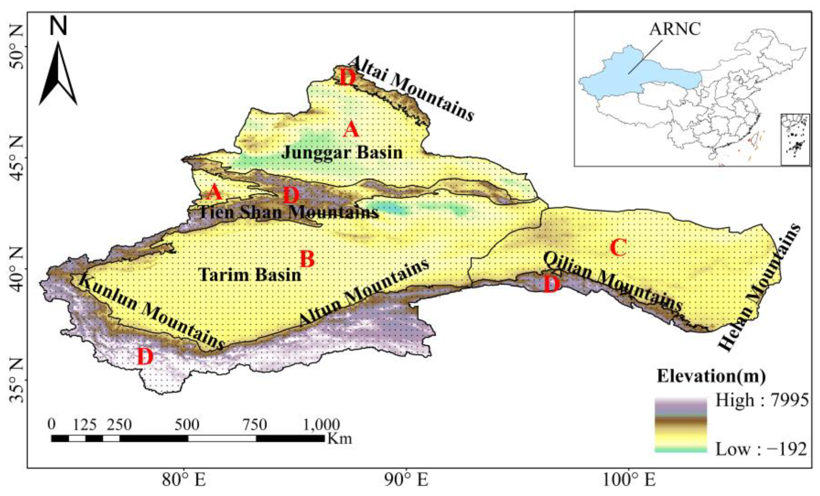
2.1. Study Area

The ARNC is located in the center of Eurasia with a latitude of 34° N–48° N and longitude of 73° E–108° E, covering the whole of Xinjiang, the west of Gansu province and the western part to the Helan Mountains in Inner Mongolia. It has a typical temperate continental climate with low precipitation, sufficient sunshine, large interannual temperature variations and dry climate. Due to the wide geographical distribution, the topography and landforms are very complex. The most prominent geomorphological feature is the distribution of basins and mountains. From north to south, the Altai Mountains, Junggar Basin, Tien Shan Mountains, Tarim Basin, Kunlun Mountains, Altun Mountains, Qilian Mountains and Helan Mountains in the east are distributed in order. There are large differences in elevations between high mountains and low basins, resulting in great spatial differences of climate elements. Thus, except for the whole ARNC, four subregions were divided according to elevation, terrain and administrative boundaries, that is, north of Xinjiang, south of Xinjiang, Hexi corridor and mountain area (Figure 1). The specific considerations for region division include three aspects. First, the ARNC is divided into Xinjiang and the whole Hexi corridor according to the administrative boundaries of Xinjiang. Then, according to the topography of Xinjiang, Xinjiang is divided into the Altai Mountains, Tien Shan Mountains, Kunlun Mountains, Junggar Basin and Tarim Basin. Finally, the area where the elevation is higher than 2400 m in the Hexi corridor, Altai Mountains, Tien Shan Mountains and Kunlun Mountains are merged to form a single region—the mountain area.

2.2. Materials

The monthly model data (tas, tasmax and tasmin) were obtained from the historical runs of 29 CMIP6 models for r1i1p1f1, covering the period from 1850 to 2014. The basic information regarding the models is shown in Table 2 (https://esgf-node.llnl.gov/search/cmip6/, accessed on 5 April 2021). Considering the different resolutions of data from different models, the simulation data were uniformly interpolated to the same grid with 0.25° latitude by 0.25° longitude as the observation data using bilinear interpolation method to facilitate the comparison.
The monthly gridded dataset, CN05.1, was used as the reference observation data. It is provided by the National Climate Center of China Meteorological Administration and was interpolated based on daily observation data from more than 2400 Chinese surface meteorological stations. The spatial resolution is 0.25° × 0.25° and the time scale is 1961–2020 [34]. In order to ensure the consistency of model data and observation data in time, 1961–2014 was selected as the evaluation period in this study.

2.3. Methods

Five methods were used to analyze and evaluate the models.
(1) The Pearson correlation analysis. It was applied to evaluate the time series correlation of model simulation data and observation data.
(2) Unitary linear regression. It was used to calculate the trend of climate change.
(3) The Taylor diagram [35]. The normalized Taylor diagram was employed to evaluate the model’s simulation ability in expressing the similarity of the spatial distribution between the simulated field and the observed field through three indices: the correlation coefficient (CC), the ratio of standard deviation (RSD) and the normalized centered root-mean-square error (CRMSE). Among them, the radial distance from the origin to the point represents the ratio of standard deviation (i.e., normalized standard deviation), while the azimuthal position gives the correlation coefficient between the simulated field and the observed field. CRMSE is the distance between observation data and model data, represented in the Taylor diagram as a dashed green semicircular arc with the observation (Obs) as the center of the circle. The larger the CC is, the smaller the CRMSE is, and the closer the RSD is to 1, the better the simulation ability of the model is.
(4) Model ranking. Using the three evaluation indices in the Taylor diagram (CC, RSD and CRMSE) to calculate the rating indices, one can use model ranking to judge the consistency of evaluation indices and obtain the comprehensive model ranking (MR) in simulating climate mean field. The MR [36,37] is defined as follows:
M R = 1 1 1 × n × m   i = 1 n R i  
where m is the number of CMIP6 models, and m = 29 in this paper; n is the number of indices participating in the evaluation, n = 3; Ri is the ranking of each model, and the model with the strongest simulation ability has an Ri of 1. The closer the MR is to 1, the better the simulation ability of the model is.
(5) Model ensemble and preferred-model selection. The equal-weight multi-model ensemble (MME) is the mean of all 29 individual models, and the equal-weight preferred-model ensemble (PME) is the mean of selected models with better simulation ability (named the preferred model). The criteria for selecting the preferred model in this study are as follows. First, the CC of time series should pass the significance level of 0.01 [38]. Second, the simulated trend should be within the range of plus or minus 30% of the observed trend and also pass the significance level of 0.01 [39]. Third, the MR should be in the top 50%, and CRMSE should be less than 1. In addition, if there are multiple GCMs meeting the above conditions and they are from the same institution, only one model with the best performance is selected to participate in the PME to reduce the unilateral influence of models from the same institution. The preferred-model selection is carried out before the ensemble to reduce the effect of ‘bad’ models on the whole as well as lessen the workload of ensemble and the high requirements for running space [40,41].

3. Results and Analysis

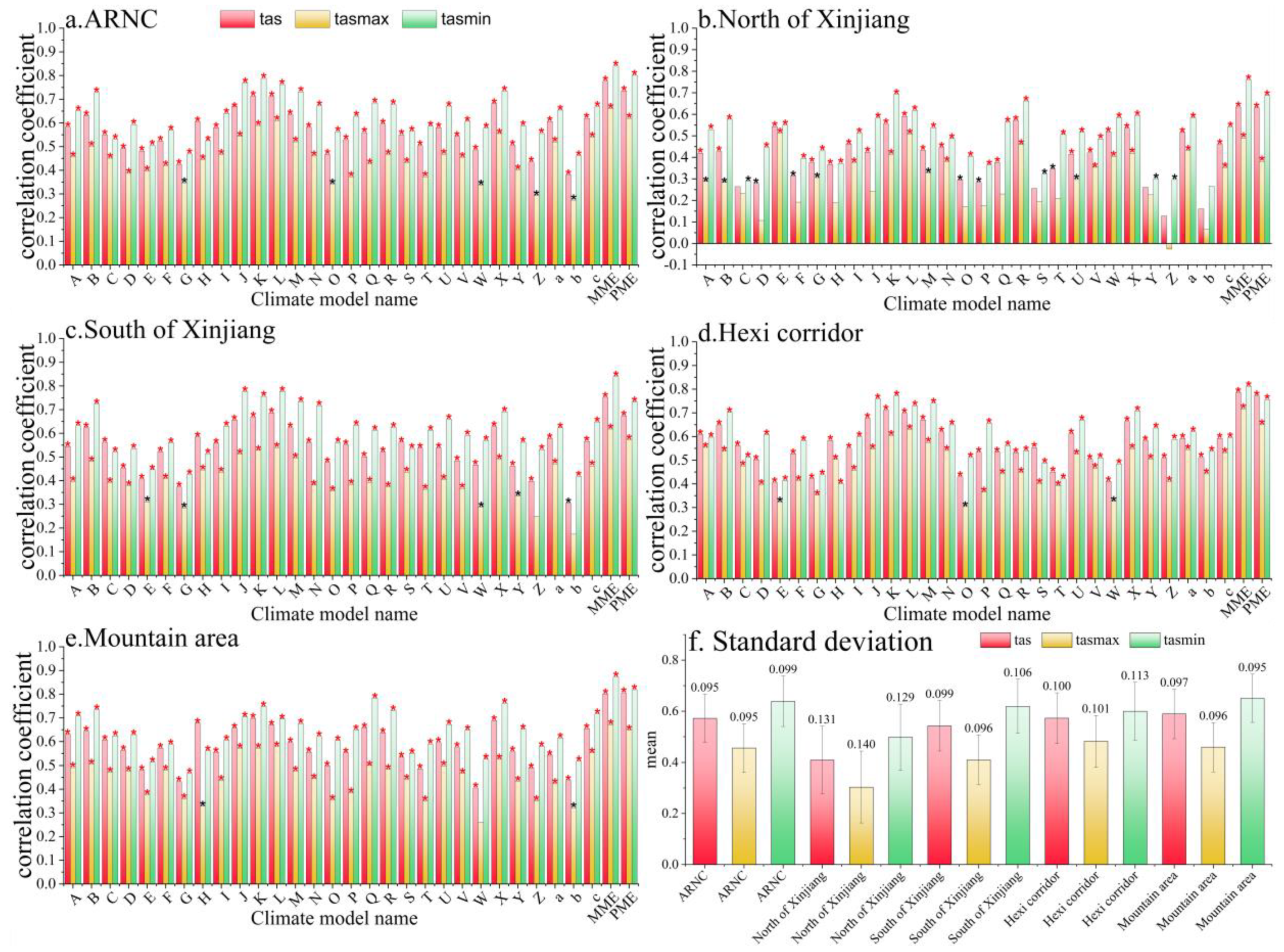
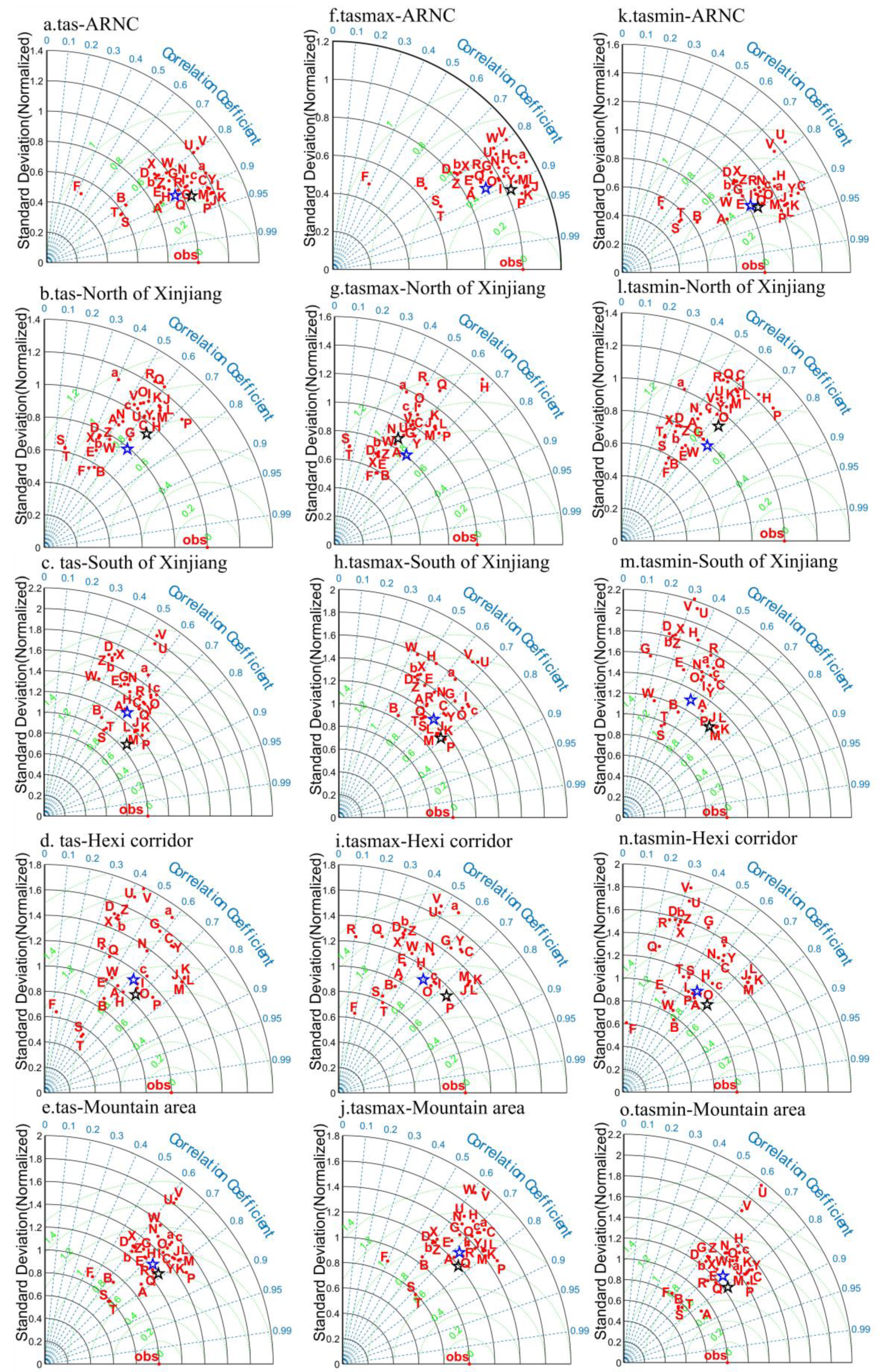
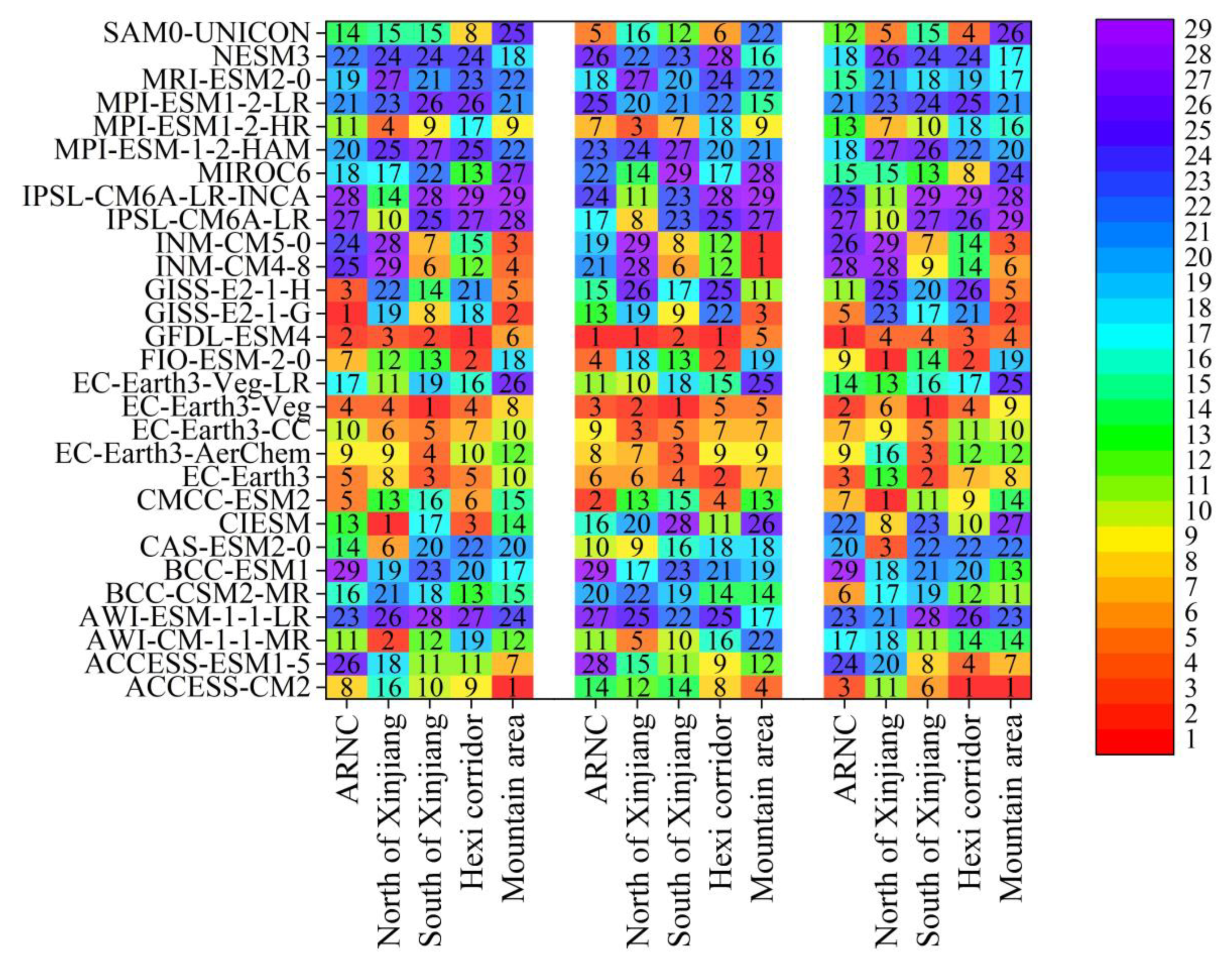
3.1. Assessment Based on Time Series Correlation

The CC between simulated data and observed data for the three temperature elements (Figure 2a–e) show that most of the models have good correlation at the significance level of 0.01. Except for the north of Xinjiang (Figure 2b), at least 23 models pass the 0.01 significance level in the other subregions.
The simulation results of the individual models are generally consistent, but the performance of each model varied in different region. Overall, nine models (I, K, L, N, R, V, X, a and c, see Table 2 for details) exhibit good correlation for the three temperature elements in all regions (p < 0.01). Among them, model K and L have the highest correlation, with CC between 0.41 and 0.79 (p < 0.01), and model b has the lowest correlation, with CC between 0.06 and 0.53. Some models have lower CC with observed data in the north of Xinjiang but a better CC in other regions, such as model C, S, Y, Z and b, with the CC being less than 0.3 in most areas. The individual models have the worst simulation effect for tasmax in northern Xinjiang (Figure 2b), and 13 models failed to pass the significance level of 0.05, and one of them has negative correlations (r = −0.026). The CCs of tasmax simulated by model J and Q exceed 0.38 (p < 0.01) for all regions except for northern Xinjiang, where the highest CC is only 0.24 (p < 0.1). Overall, the CC between model and observation data is better for tas and tasmin and slightly lower for tasmax. All of these results show the importance of regional discussion.
For the multi-model ensemble mean, the CCs between MME and observations are larger than that of individual models in all subregions except for tasmax in the north of Xinjiang. The reason for this is possibly that the number of models with a better CC in the north of Xinjiang is less than that in other subregions and the whole ARNC. Although the CC of MME for tasmax in the north of Xinjiang is smaller than that of model E and L, its CC is still as high as 0.49 (p < 0.01) (Figure 2b).
The standard deviation and mean of correlation coefficients for the three temperature elements in the ARNC and subregions are shown in Figure 2f. Overall, the correlation of tasmin is the highest, with the mean values of CC exceeding 0.5 in all regions, while tasmax has the lowest correlation, with the mean values of CC ranging from 0.30 to 0.48. Regionally, the models show relatively poor correlations in the north of Xinjiang for the three temperature elements, but the best in mountain areas for tas and tasmin. The standard deviation of CC in the north of Xinjiang is larger than that in other regions, but there is little difference among the three temperature elements.

3.2. Assessment Based on Long-Term Trend Simulation

In terms of tas, the warming trend of Hexi corridor is obviously higher than that of ARNC and other subregions, with a warming rate of 0.35 °C/10 a (Figure 3d). The trend simulated by model I, L, O and R is closest to the observed value in the ARNC (0.30 °C/10 a), north of Xinjiang (0.32 °C/10 a) and mountain area (0.30 °C/10 a), with the deviation within 0~0.02 °C/10 a. In south of Xinjiang, the simulated trend by model C and R (0.26 °C/10 a) is closest to the observed value (0.255 °C/10 a), while in the Hexi corridor, model B (0.33 °C/10 a) has the closest value to the observed one (0.35 °C/10 a). In particular, model R can effectively capture the warming trend of the other three regions, except for the Hexi corridor, which has a deviation of 0.06 °C/10 a.
Regarding tasmax, the observed trends in the ARNC, north of Xinjiang, south of Xinjiang, Hexi corridor and mountain area are 0.22 °C/10 a, 0.20 °C/10 a, 0.20 °C/10 a, 0.28 °C/10 a and 0.23 °C/10 a, respectively (Figure 3). The change rates simulated by model C and Z are closer to the observed ones in the ARNC and north of Xinjiang, with the deviation ranging 0~0.02 °C/10 a. In southern Xinjiang, model N and Y have the best simulated change trend. For the Hexi corridor and mountain area, model M is closest to the observed values. It is worth noting that the long-term trend simulated by model W is the worst in the Hexi corridor and south of Xinjiang, failing to pass the significance test of 0.05, with the deviation of 0.16 °C/10 a.
Compared to tas and tasmax, tasmin has the most obvious warming rate, with the observed trend ranging from 0.39 °C/10 a to 0.49 °C/10 a in the ARNC and its subregions (p < 0.01). In the mountain area, the simulated trends by all individual models and the MME are lower than the observed ones. In the north of Xinjiang (model J), south of Xinjiang (model M and U) and the mountain area (model J and K), these models have the closest simulated values to the observed ones. The change rates simulated by model U are closer to the observed one in the ARNC and Hexi corridor, with the deviation ranging 0–0.02 °C/10 a.
In general, trends of the three temperature elements all show a significant upward trend. Among them, tasmin has the highest upward trend, and tasmax has the lowest upward trend, which can be effectively simulated by most models, but the intensity of the simulated trend varies greatly among models. The majority of the 29 models pass the significance level of 0.01. Overall, the warming rates for tasmin simulated by the models are lower than that of the observed, with the deviation ranging from −0.153 to −0.077 °C/10 a (Figure 3f). Except for the Hexi corridor, the models overestimate the warming rate for tasmax, with a deviation of 0.02~0.07 °C/10 a (Figure 3f). The standard deviation of the simulated trend is lower for tas than for tasmin and tasmax in all regions. Regionally, the standard deviations of simulated trends are higher in the Hexi corridor than in other regions for the three temperature elements. Moreover, the MME still underestimates the temperature change trend for tasmin and tas. In capturing the variation of temperature, the performance of the MME is not as good as often as those by individual models, which is consistent with previous studies [5,39].

3.3. Assessment Based on Spatial Pattern Simulation

The Taylor diagram was used to evaluate the ability of CMIP6 models in simulating the mean field of temperature during 1961–2014 (Figure 4). On the whole, the 29 models and MME have a certain simulation ability to reproduce the climate average state of the three temperature elements but vary in different subregions.
In the ARNC, the models have good simulations for tas (Figure 4a), tasmax (Figure 4f) and tasmin (Figure 4k). The spatial CC between simulation field and observation field for most models range between 0.70 and 0.95, the CRMSE is less than 0.8, and the RSD is distributed between 0.8 and 1.2. Except for tasmin, whose RSD are a little bit scattered, the other elements are consistent, indicating that most models have the consistent simulation for the three temperature elements, which can be shown by the concentrated distribution in the Taylor plots. The MME can effectively capture the spatial pattern of ARNC, with the spatial CC close to 0.9.
In the north of Xinjiang, the simulation effects of the individual models for the three temperature elements are relatively close, with the spatial CC between 0.4 and 0.7, the CRMSE of 69% of models less than 1 and the RSD between 0.6 and 1.2, indicating that the spatial standard deviations of most models are smaller than those observed in the north of Xinjiang. In the south of Xinjiang, the individual models cannot simulate climate mean fields well. The RSD and CRMSE of most models are greater than 1. Among them, model F (BCC-ESM1) performs worst, showing a negative correlation with the observation field. For the convenience of model comparison and graphic display, model F is not shown in figures (Figure 4c,h,m). The simulation of the three temperature elements in the Hexi corridor by each model is similar to that in the south of Xinjiang. The difference is that the spatial CC in the Hexi corridor is positive, and its RSD is more scattered. For the mountain area, the simulation by the individual models is slightly better than that in the south of Xinjiang and the Hexi corridor. Notably, models S and T can better reproduce the spatial distribution of the temperature elements in the Hexi corridor and mountain area, but reproduction is worse in other subregions.
Overall, the spatial pattern simulated by the 29 models is best in the ARNC and the north of Xinjiang, but poor in the other subregions. The MME performs well in each region and outperforms most individual models, with the spatial CC between 0.50 and 0.89, the CRMSE within 0.47~1.19 and the RSD between 0.79 and 1.31.
Figure 5 shows the 29 models’ comprehensive ranking of simulation ability in simulating the climate mean field of the three temperature elements in the ARNC and subregions. According to the MR of the three elements in each region, models with better simulation performance are obtained, such as EC-Earth3 (J), EC-Earth3-Aerchem (K), EC-Earth3-CC (L), EC-Earth3-Veg (M) and GFDL-ESM4 (P). Meanwhile, the models with poor simulation ability are also obtained, such as AWI-ESM-1–1-LR (D), BCC-ESM1 (F), MPI-ESM-1-2-HAM (X), MPI-ESM1-2-LR (Z) and NESM3 (b).

3.4. Assessment Based on Preferred Models

Based on the evaluation results of the above three aspects, the models with better simulation ability (named the preferred model) were selected to form the preferred-model ensemble (PME) according to the criteria stated in the Methods section. The preferred models for ARNC and each subregion are shown in Table 3. It can be noticed that there are multiple models meeting the criteria in some regions, while only a few in other regions.

3.4.1. Simulation Effect of PME on Time Series Correlation, Trend Magnitude and Spatial Pattern

Figure 2 shows that the CC of the PME is largely consistent with that of the MME, both passing the significance test of 0.01, with the CC ranging from 0.38 to 0.82. For tasmax, the CC of the PME is higher than those of individual models except for the north of Xinjiang. For tas and tasmin, the CC of the PME is less than mode L(EC-Earth3-CC) in the south of Xinjiang, but still higher than the other models.
The error range of trend is −0.16~0.08 °C/10 a and −0.07~0.01 °C/10 a for the MME and PME, respectively (Figure 3). Especially in the south of Xinjiang, the error is only 0.01 °C/10 a for the PME, indicating that the PME outperforms the MME in long-trend simulation. Even so, the simulated warming rate for tasmin by the PME is still low, which needs further correction to reduce the uncertainty of model simulation in the future.
The mean field of three temperature elements in the ARNC and subregions simulated by the PME are shown in Figure 4 by the Taylor diagram. The results demonstrate that the MME and PME exhibit better simulation performance for climate mean fields than individual models, with the PME outperforming the MME. The spatial CCs of the PME for all three temperature elements in all regions vary from 0.53 to 0.91, while those of the MME ranges from 0.50 to 0.89. Meanwhile, the RSD of the PME is 0.91~1.27, and the CRMSE is 0.42~0.92. In the north of Xinjiang, the RSD of the PME is greatly improved, and the result is close to 1, showing that the standard deviation of the PME is basically consistent with that observed. This indicates that selecting a better model contributes to the improvement of the ensemble mean simulation, which is consistent with the findings of some previous studies [42].

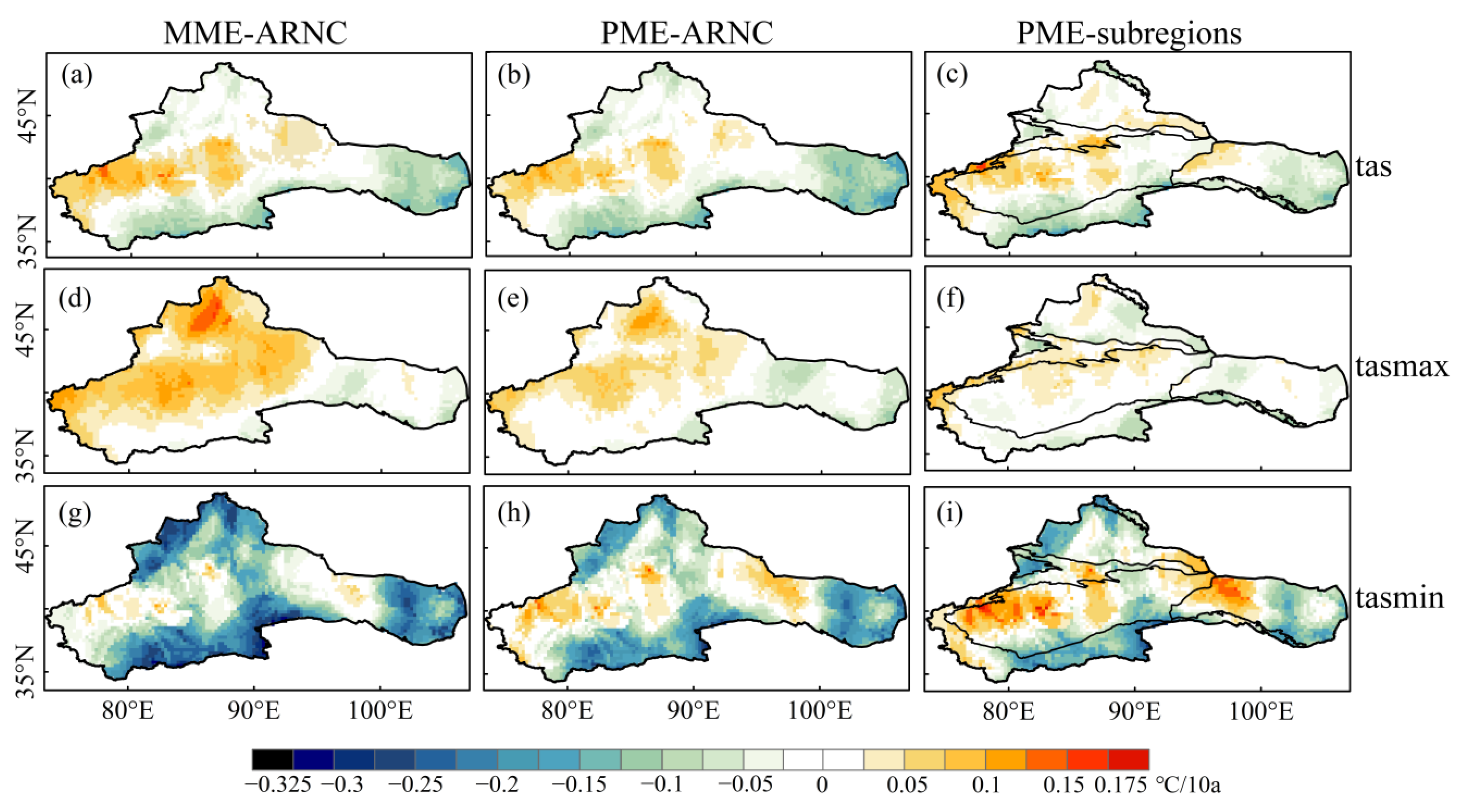
3.4.2. Simulation Effect of PME on Temperature Spatial Change Trend

The spatial deviation of trends between the simulations by the two ensemble means (MME and PME) and the observations are shown in Figure 6. For tas, the MME overestimates temperature trends in the north and west of southern Xinjiang (Figure 6a), with a bias of about 0.1 °C/10 a, while the PME significantly reduces this bias to 0.075 °C/10 a. Furthermore, the range and the distribution area of the warm bias in the eastern Hexi corridor are significantly reduced after area partition compared to the whole ARNC. For tasmax, the temperature trend in Xinjiang is overestimated by the MME, with a deviation of 0.075~0.25 °C/10 a, while both the PME and PME-subregions reduce the deviation to 0.025~0.1 °C/10 a in Xinjiang. At the same time, both the MME and PME can better capture temperature spatial change trends in the Hexi corridor. For tasmin, the MME severely underestimates the temperature trends in northern Xinjiang, the mountain area and the eastern Hexi corridor, with deviations of about 0.275 °C/10 a (Figure 6g). Compared with the MME, the PME significantly reduces the range of deviation in the north of Xinjiang and the mountain area.
In general, the PME outperforms the MME in reproducing the spatial distribution of the temperature change trend in ARNC. For tas and tasmax, the PME can significantly reduce the trend deviation after area partition in all regions.

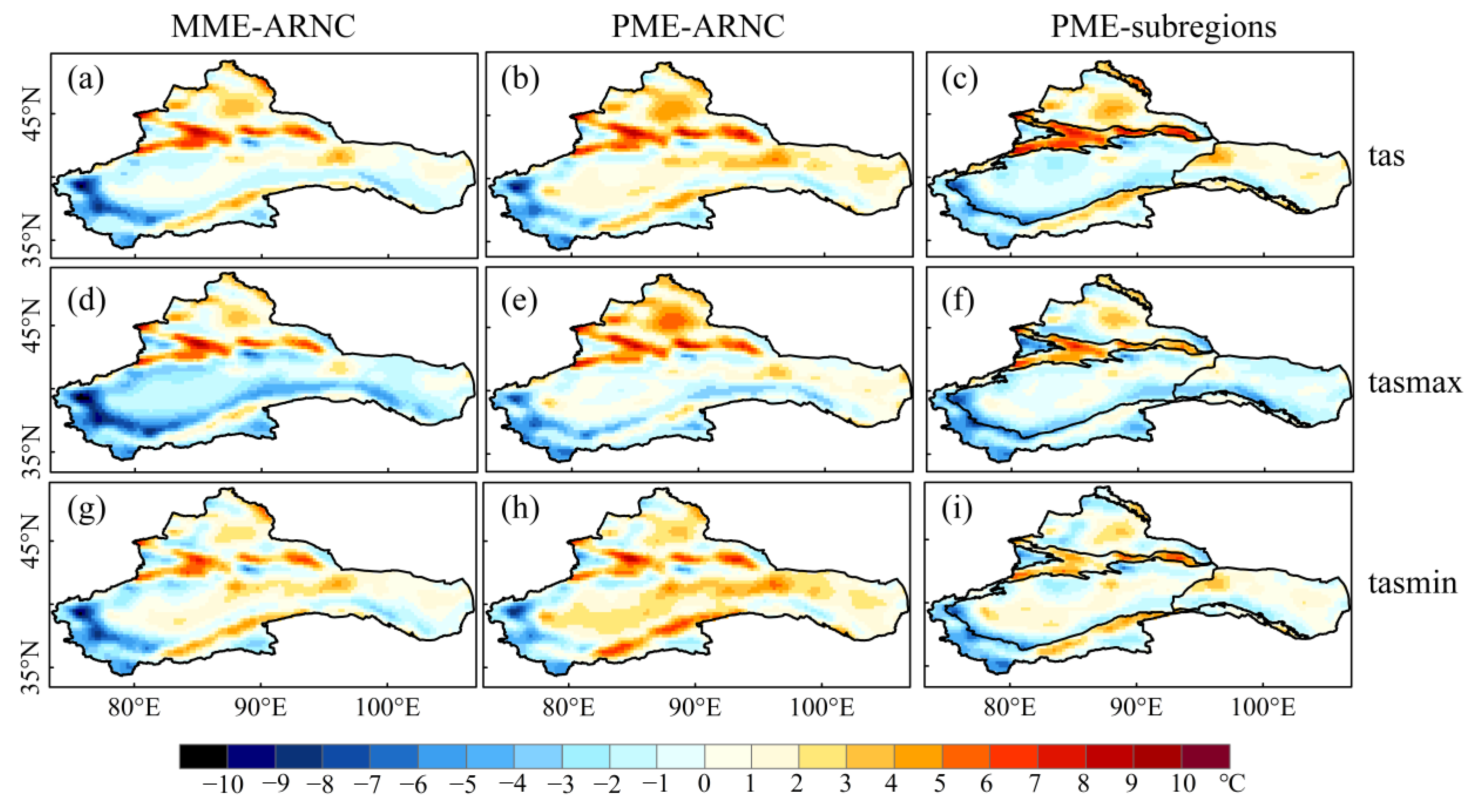
3.4.3. Simulation Effect of PME on Temperature Spatial Distribution

The deviation distribution of the three temperature elements simulated by the two ensemble means (MME and PME) shows that the MME has a warming bias of about 3 °C for tas and tasmax, which is slightly lower than that of the PME (Figure 7) in the north of Xinjiang. The possible reason for this is that there are fewer preferred models, and the spatial simulation performance of the individual models is poor, lowering the overall level. For tasmin, the simulation deviation of the PME after partition is consistent with the spatial distribution of the MME.
The MME has a cold deviation of 3~4 °C for tasmax in the south of Xinjiang, while the PME reduces this deviation to −1~1 °C. In the Hexi corridor, the spatial distribution of three temperature elements simulated by the PME and MME is approximately the same, and the deviation from the observed temperature is within ±2 °C. In the mountain area, the deviation of tasmin simulated by the PME after partition is 1~3 °C lower than that of the MME (2~5 °C) in the Tien Shan Mountains and Altun Mountains. In the Kunlun Mountains, the deviations of the PME are significantly lower than those of the MME for the three temperature elements.
Generally, compared with the MME, the PME can better simulate the spatial distribution of tas, tasmax and tasmin in the ARNC, except for the north of Xinjiang, and reduce the deviation to some extent.

4. Discussion

Solving the uncertainty of model simulation has been a hot topic in the application of GCMs for the simulation and prediction of regional climate change. On the one hand, the simulation accuracy needs to be improved from the model itself so that it can be better applied to regional-scale simulations. On the other hand, methodological improvements can likewise boost the credibility of the model. Based on HadEX3 observations and four reanalysis datasets, Kim et al. evaluated the capability of CMIP6 to simulate global climate extreme indices using root-mean-square errors and found that the performance of the multi-model ensemble mean outperformed that of the individual models [43]. Combined with the results of this paper, the MME can reproduce the spatial and temporal characteristics of temperature better than individual models, especially the PME, which displays better performance. This suggests that the ensemble mean, as a consensus between multiple models, does help eliminate uncertainty caused by internal variability among models and is a way to improve the reliability of model simulations [44,45].
The current research results indicate that the CMIP6 model has a better ability to simulate climate than CMIP5 [46,47]. For example, CMIP6 can minimize the temperature deviation to 1.08 °C from 1.52 of CMIP5 [48] in simulating the temperature and precipitation of the Qinghai–Tibet Plateau. In addition, the CMIP6 models are found to be definitely improved in simulating the annual average temperature in the ARNC compared to the CMIP5. In terms of the correlation coefficient between simulation and observation for each model, about 64% (25 out of 39) of CMIP5 models passed the significance test of 0.01 in the ARNC [49], while all the CMIP6 models (29 out of 29) do in our study. In terms of the long-term trend simulation, about 25% (10 out of 39) of CMIP5 models had a deviation less than 0.03 °C/10 a [49], while approximately 41% (12 out of 29) CMIP6 models do in our study.
In comparison to previous research, this report focuses more on which models perform better in subregions. Although some studies [13,16,37,50] have also investigated the performance of CMIP6 GCMs in simulating air temperature, little attention has been paid to the model performance disparities between subregions and the whole of study areas. The majority of research did not select better models for each subregion, but only simply evaluated models over the whole area, which may produce errors at smaller regional scales and affect the reliability of future prediction results. Through the comparison of the PME-ARNC and PME-subregions in Figure 7 of this paper, we found that the better model selected separately for each subregion can indeed reduce the simulation bias, which is also reflected in Figure 6. While selecting the better model for the whole of the ARNC improves simulation capacity, it does not necessarily eliminate bias in smaller regions more precisely, which is consistent with earlier studies [51,52].
Through the analysis and comparison, the preferred model for each subregion and each temperature element were pointed out (Table 3) in this paper, which could provide a reference for model users. For example, model A is better for tasmin, model H is better for tas, but models D and E are not good for the three temperature elements as a whole. Why do the models perform so differently? In this paper, we found that the models with better simulation in space and time generally have a higher spatial resolution, such as EC-Earth3, EC-Earth3-CC, EC-Earth3-Veg and GFDL-ESM4, which is also consistent with previous studies [32,37,53]. In contrast, models with lower resolution, such as BCC-ESM1, NESM3 and AWI-ESM-1-1-LR, have poor simulation ability in the ARNC and subregions. Furthermore, the different parameterization schemes and external forcing of the model itself will also make the models have different performances. Some previous studies have shown that models with the same resolution do not mean they have the same simulation capability [54,55]. In this study, we conducted a simple comparison of model simulation ability, without involving in-depth comparison, such as internal physical processes, external forcing factors, etc., which are directions to be explored in the future.
The same model has different simulation capabilities in different regions [56,57]. In this paper, the model has an obvious warm deviation for the Tien Shan Mountains and an obvious cold deviation for the Kunlun Mountains, while it is better for the Hexi corridor (Figure 7). The reason for this difference may be related to the different underlying surface conditions. In the mountain area, where the topography is more complex and the altitude is higher, the simple interpolation of the model may not be able to capture the change in air temperature at different elevations [58]. In contrast, the underlying surface of the Hexi corridor is homogeneous and the topographic relief is smaller, leading to the model having better simulations. In addition, the circulation condition is also an important factor causing the different performances of models. The ARNC is in the area influenced by the prevailing westerly winds in the west and the East Asian summer winds in the eastern part [59]. The change in circulation over the Qinghai–Tibet Plateau, located next to the ARNC, is closely related to the climate of China’s arid area. The dynamic and thermal effects of the Qinghai–Tibet Plateau will have an impact on the ARNC [60,61]. As described by Monerie et al. [62], model differences lie in how the models simulate changes in atmospheric circulation patterns.
Due to the special geographical location and complex topographic features in the ARNC, the response of different regions to climate change is various and sensitive. In this paper, the trend of increasing surface mean temperature in the ARNC is 0.30 °C/10 a from 1961 to 2014, which is higher than the values worldwide and in China [63], and also higher than those of the global arid zone from 1961 to 2018 (0.21 °C/10 a). Continuous increases in air temperature will accelerate the melting and retreat of glaciers, change the composition of runoff and aggravate the fluctuation of water resources. In rivers mainly fed by glaciers and snow in the ARNC, such as the Yarkant River, Hotan River and Shule River, increases in meltwater have been observed [64,65]. Additionally, the rising temperature will have an impact on evapotranspiration. Studies have shown that there is a consequent change of 19.34 mm in evapotranspiration for every 1 °C increase in temperature for global land [66]. All of this indicates that it is imperative to carry out regional climate simulation and projection and pay especially close attention to changes in extreme climate.
Although the simulation effect of the PME has been proved to be better than both the MME and most individual models, it should be noted that the PME still underestimates the warming rate of tasmin. It could be improved by correcting the deviation of models or assigning different weights to the models. In addition, the use of high-resolution regional climate models (e.g., RegCM2, WRF, CCLM, etc.) or proper downscaling methods are also solutions.

5. Conclusions

Based on the monthly temperature observation data of CN05.1 and the simulation data of CMIP6 models, we evaluated the ability of 29 individual models and model ensembles (MME and PME) in simulating tas, tasmax and tasmin in the ARNC and subregions during 1961–2014. The preliminary conclusions are summarized as follows.
(1) The 29 CMIP6 models have a certain simulation ability in reproducing the characteristics of temporal trends and spatial patterns of temperature elements in the ARNC. Except for tas and tasmax in the north of Xinjiang, the CCs between simulations and observations for more than 79% of the models pass the significance test of 0.01. The MME outperforms the individual models in simulating correlations of time series, with the CC ranging from 0.49 to 0.87 (p < 0.01).
(2) Based on the observations, the three temperature elements show a warming trend in the ARNC and subregions from 1961 to 2014, and the warming rate behaves as tasmin > tas > tasmax, with the lowest one in the south of Xinjiang among all regions, indicating that the annual mean minimum temperature has the strongest warming effect on the whole climate system of the ARNC. The warming rate simulated by most models (>85%) is generally lower than the observed ones for tasmin, and only a few models can effectively simulate the temperature trends in each region. The MME is not better than individual models in simulating the change trend of three temperature elements.
(3) Most of the models can simulate the mean field of the three temperature elements better, but the simulation ability varies among regions. On the whole, the simulation effect is better in the ARNC and the north of Xinjiang and worse in the Hexi corridor and the mountainous area. The spatial CCs all exceed 0.7 in the ARNC. The model F (BCC-ESM1) has poor simulation in all regions. The MME is better than the individual models in showing the spatial pattern of climate mean field.
(4) The preferred models for each region and each temperature element are pointed out in Table 3. Compared with the 29 individual models and the MME, the PME consisting of preferred models significantly improves the ability to simulate both the change trend and the spatial patterns of climate mean field. The temporal and spatial correlation coefficients of the PME range from 0.38 to 0.82 and 0.53 to 0.91, respectively. The PME is more stable than the MME in simulation. Moreover, the error range of the long-term trend is only −0.07~0.01 °C/10 a for the PME. The PME, especially PME-subregions, can obviously reduce the deviation range of the temporal and spatial change trend and clearly reproduce the temperature spatial distribution in the Hexi corridor and the mountain area.

Author Contributions

Conceptualization, C.X.; Methodology, Y.L. and F.L.; Software, G.Y. and H.W.; Validation, F.L. and Y.L.; Formal Analysis, F.L. and C.X.; Writing—Original Draft Preparation, F.L. All authors have read and agreed to the published version of the manuscript.

Funding

This work was supported by the National Natural Science Foundation of China (No. 42067062). The funder is Changchun Xu and the funding number is 42067062.

Institutional Review Board Statement

Not applicable.

Informed Consent Statement

Not applicable.

Data Availability Statement

The CN05.1 data are available from Xu et al. The data of CMIP6 models are from https://esgf-node.llnl.gov/search/cmip6/, accessed on 5 April 2021.

Conflicts of Interest

The authors declare no conflict of interest.

References

  1. Solomon, S.D.; Qin, D.; Manning, M.; Chen, Z.; Miller, H.L. Climate Change 2007: The Physical Science Basis. Working Group I Contribution to the Fourth Assessment Report of the IPCC; Cambridge University Press: Cambridge, UK; New York, NY, USA, 2007. [Google Scholar]
  2. Seneviratne, S. Changes in climate extremes and their impacts on the natural physical environment: An overview of the IPCC SREX report. In A Special Report of Working Groups I and II of the Intergovernmental Panel on Climate Change; Cambridge University Press: Cambridge, UK; New York, NY, USA, 2012. [Google Scholar]
  3. IPCC; Stocker, T.F.; Qin, D.; Plattner, G.K.; Midgley, P.M. IPCC, 2013: Climate Change 2013: The Physical Science Basis. Contribution of Working Group I to the Fifth Assessment Report of the Intergovernmental Panel on Climate Change; Cambridge University Press: Cambridge, UK; New York, NY, USA, 2013. [Google Scholar]
  4. Zhang, Y.; Zhang, L.; Xu, Y. Simulations and Projections of the Surface Air Temperature in China by CMIP5 Models. Clim. Change Res. 2016, 12, 10–19. [Google Scholar] [CrossRef]
  5. Wu, J.; Wang, B.; Yang, Y.; Chang, Y.; Chen, L.; Yang, J.; Liu, X. Comparing Simulated Temperature and Precipitation of CMIP3 and CMIP5 in Arid Areas of Northwest China. Clim. Change Res. 2017, 13, 198–212. [Google Scholar] [CrossRef]
  6. Xu, L.; Wang, A.; Yu, W.; Yang, S. Hot spots of extreme precipitation change under 1.5 and 2 °C global warming scenarios. Weather. Clim. Extrem. 2021, 33, 100357. [Google Scholar] [CrossRef]
  7. Sonali, P.; Kumar, D.N.; Nanjundiah, R.S. Intercomparison of CMIP5 and CMIP3 simulations of the 20th century maximum and minimum temperatures over India and detection of climatic trends. Theor. Appl. Climatol. 2017, 128, 465–489. [Google Scholar] [CrossRef]
  8. Papadimitriou, L.; Koutroulis, A.G.; Tsanis, I.K.; Grillakis, M.G. Evaluation of precipitation and temperature simulation performance of the CMIP3 and CMIP5 historical experiments. Clim. Dyn. 2016, 47, 1881–1898. [Google Scholar] [CrossRef]
  9. Gao, Y.; Wang, H.; Jiang, D. An intercomparison of CMIP5 and CMIP3 models for interannual variability of summer precipitation in Pan-Asian monsoon region. Int. J. Climatol. 2015, 35, 3770–3780. [Google Scholar] [CrossRef]
  10. Zhou, T.; Zou, L.; Chen, X. Commentary on the Coupled Model Intercomparison Project Phase 6 (CMIP6). Clim. Change Res. 2019, 15, 445–456. [Google Scholar] [CrossRef]
  11. Zhang, L.; Chen, X.; Xin, X. Short commentary on CMIP6 Scenario Model Intercomparison Project (ScenarioMIP). Clim. Change Res. 2019, 15, 519–525. [Google Scholar] [CrossRef]
  12. Stouffer, R.J.; Eyring, V.; Meehl, G.A.; Bony, S.; Senior, C. CMIP5 Scientific Gaps and Recommendations for CMIP6. Bull. Am. Meteorol. Soc. 2017, 98, 95–105. [Google Scholar] [CrossRef]
  13. Ayugi, B.; Ngoma, H.; Babaousmail, H.; Karim, R.; Ongoma, V. Evaluation and projection of mean surface temperature using CMIP6 models over East Africa. J. Afr. Earth Sci. 2021, 181, 104226. [Google Scholar] [CrossRef]
  14. Fan, X.; Duan, Q.; Shen, C.; Wu, Y.; Xing, C. Global surface air temperatures in CMIP6: Historical performance and future changes. Environ. Res. Lett. 2020, 15, 104057. [Google Scholar] [CrossRef]
  15. Cui, T.; Li, C.; Tian, F. Evaluation of Temperature and Precipitation Simulations in CMIP6 Models Over the Tibetan Plateau. Earth Space Sci. 2021, 8, e2020EA001620. [Google Scholar] [CrossRef]
  16. Yang, X.; Zhou, B.; Xu, Y.; Han, Z. CMIP6 Evaluation and Projection of Temperature and Precipitation over China. Adv. Atmos. Sci. 2021, 38, 817–830. [Google Scholar] [CrossRef]
  17. Zhu, H.; Jiang, Z.; Li, J.; Li, W.; Sun, C.; Laurent, L.I. Does CMIP6 Inspire More Confidence in Simulating Climate Extremes over China? Adv. Atmos. Sci. 2020, 37, 1119–1132. [Google Scholar] [CrossRef]
  18. Lin, W.; Chen, H. Assessment of model performance of precipitation extremes over the mid-high latitude areas of Northern Hemisphere: From CMIP5 to CMIP6. Atmos. Ocean. Sci. Lett. 2020, 13, 598–603. [Google Scholar] [CrossRef]
  19. Srivastava, A.; Grotjahn, R.; Ullrich, P.A. Evaluation of historical CMIP6 model simulations of extreme precipitation over contiguous US regions. Weather. Clim. Extrem. 2020, 29, 100268. [Google Scholar] [CrossRef]
  20. Chen, C.; Hsu, H.; Liang, H. Evaluation and comparison of CMIP6 and CMIP5 model performance in simulating the seasonal extreme precipitation in the Western North Pacific and East Asia. Weather. Clim. Extrem. 2021, 31, 100303. [Google Scholar] [CrossRef]
  21. Gupta, V.; Singh, V.; Jain, M.K. Assessment of precipitation extremes in India during the 21st century under SSP1-1.9 mitigation scenarios of CMIP6 GCMs. J. Hydrol. 2020, 590, 125422. [Google Scholar] [CrossRef]
  22. Yao, J.; Yang, Q.; Chen, Y.; Hu, F.; Liu, Z.; Zhao, L. Climate change in arid areas of Northwest China in past 50 years and its effects on the local ecological environment. Chin. J. Ecol. 2013, 32, 1283–1291. [Google Scholar] [CrossRef]
  23. You, Q.; Kang, S.; Pepin, N.; Yan, Y. Relationship between trends in temperature extremes and elevation in the eastern and central Tibetan Plateau, 1961–2005. Geophys. Res. Lett. 2008, 35, 317–333. [Google Scholar] [CrossRef] [Green Version]
  24. Yao, X.; Zhang, M.; Zhang, Y.; Wang, J.; Xiao, H. New understanding of climate transition in nortnwest China. Arid. Land Geogr. 2021. online. [Google Scholar]
  25. Yao, J.; Mao, W.; Chen, J.; Dilinuer, T. Signal and impact of wet-to-dry climatic shift over Xinjiang, China. Acta Geogr. Sin. 2021, 76, 57–72. [Google Scholar] [CrossRef]
  26. Chen, Y.; Wang, H.; Wang, Z.; Zhang, H. Characteristics of extreme climatic/hydrological events in the arid region of northwestern China. Arid. Land Geogr. 2017, 40, 1–9. [Google Scholar] [CrossRef]
  27. Akinsanola, A.A.; Ongoma, V.; Gabriel, J.K. Evaluation of CMIP6 models in simulating the statistics of extreme precipitation over Eastern Africa. Atmos. Res. 2021, 254, 105509. [Google Scholar] [CrossRef]
  28. Almazroui, M.; Saeed, F.; Islam, M.; Khalid, M.S.; Alkhalaf, A.K.; Dambul, R. Assessment of Uncertainties in Projected Temperature and Precipitation over the Arabian Peninsula Using Three Categories of Cmip5 Multimodel Ensembles. Earth Syst. Environ. 2017, 1, 12. [Google Scholar] [CrossRef]
  29. Crawford, J.; Venkataraman, K.; Booth, J. Developing climate model ensembles: A comparative case study. J. Hydrol. 2019, 568, 160–173. [Google Scholar] [CrossRef]
  30. Jiang, W.; Chen, H. Assessment and projection of changes in temperature extremes over the mid-high latitudes of Asia based on CMIP6 models. Trans. Atmos. Sci. 2021, 44, 592–603. [Google Scholar] [CrossRef]
  31. Liu, X.; LI, C.; Zhao, T.; Han, L. Future changes of global potential evapotranspiration simulated from CMIP5 to CMIP6 models. Atmos. Ocean. Sci. Lett. 2021, 13, 568–575. [Google Scholar] [CrossRef]
  32. Bagcaci, S.C.; Yucel, I.; Duzenli, E.; Yilmaz, M.T. Intercomparison of the expected change in the temperature and the precipitation retrieved from CMIP6 and CMIP5 climate projections: A Mediterranean hot spot case, Turkey. Atmos. Res. 2021, 256, 105576. [Google Scholar] [CrossRef]
  33. Qi, Y.; Yan, Z.; Qian, C. Evaluation and projections of monthly temperature extremes over the Belt and Road region based on PDF-adjusted method. Clim. Change Res. 2021, 17, 151–161. [Google Scholar]
  34. Wu, J.; Gao, X. A gridded daily observation dataset over China region and comparison with the other datasets. Chin. J. Geophys. 2013, 56, 1102–1111. [Google Scholar] [CrossRef]
  35. Taylor, K.E. Summarizing multiple aspects of model performance in a single diagram. J. Geophys. Res. 2001, 106, 7183–7192. [Google Scholar] [CrossRef]
  36. Schuenemann, K.C.; Cassano, J.J. Changes in synoptic weather patterns and Greenland precipitation in the 20th and 21st centuries: 1. Evaluation of late 20th century simulations from IPCC models. J. Geophys. Res. 2009, 114, D20113. [Google Scholar] [CrossRef] [Green Version]
  37. Dong, T.; Dong, W. Evaluation of extreme precipitation over Asia in CMIP6 models. Clim. Dyn. 2021, 57, 1751–1769. [Google Scholar] [CrossRef]
  38. Chen, L.; Xu, C.; Li, X. Projections of temperature extremes based on preferred CMIP5 models: A case study in the Kaidu-Kongqi River basin in Northwest China. J. Arid. Land 2021, 13, 568–580. [Google Scholar] [CrossRef]
  39. Li, X.; Xu, C.; Li, L.; Luo, Y.; Yang, Q.; Yang, Y. Evaluation of air temperature of the typical river basin in desert area of Northwest China by the CMIP5 models: A case of the Kaidu-Kongqi River Basin. Resour. Sci. 2019, 41, 1141–1153. [Google Scholar] [CrossRef]
  40. Veiga, S.F.; Yuan, H.L. Performance-based projection of precipitation extremes over China based on CMIP5/6 models using integrated quadratic distance. Weather. Clim. Extrem. 2021, 34, 100398. [Google Scholar] [CrossRef]
  41. Long, Y.; Xu, C.; Liu, F.; Liu, Y.; Yin, G. Evaluation and Projection of Wind Speed in the Arid Region of Northwest China Based on CMIP6. Remote Sens. 2021, 13, 4076. [Google Scholar] [CrossRef]
  42. Zhang, X.; Li, X.; Xu, X.; Zhang, L. Ensemble projection of climate change scenarios of China in the 21st century based on the preferred climate models. Acta Geogr. Sin. 2017, 72, 1555–1568. [Google Scholar] [CrossRef]
  43. Kim, Y.H.; Min, S.K.; Zhang, X.; Sillmann, J.; Sandstad, M. Evaluation of the CMIP6 multi-model ensemble for climate extreme indices. Weather. Clim. Extrem. 2020, 29, 100269. [Google Scholar] [CrossRef]
  44. Hu, X.; Ma, J.; Ying, J.; Cai, M.; Kong, Y. Inferring future warming in the Arctic from the observed global warming trend and CMIP6 simulations. Adv. Clim. Change Res. 2021, 12, 499–507. [Google Scholar] [CrossRef]
  45. Yue, Y.; Yan, D.; Yue, Q.; Ji, G.; Wang, Z. Future changes in precipitation and temperature over the Yangtze River Basin in China based on CMIP6 GCMs. Atmos. Res. 2021, 264, 105828. [Google Scholar] [CrossRef]
  46. Zhi, H.; Huang, Y.; Lin, P.; Shi, S.; Dong, M. Interannual variability of the sea surface salinity and its related freshwater flux in the tropical Pacific: A comparison of CMIP5 and CMIP6. Atmos. Ocean. Sci. Lett. 2022, 100190. [Google Scholar] [CrossRef]
  47. Try, S.; Tanaka, S.; Tanaka, K.; Sayama, T.; Khujanazarov, T.; Oeurng, C. Comparison of CMIP5 and CMIP6 GCM performance for flood projections in the Mekong River Basin. J. Hydrol. Reg. Stud. 2022, 40, 101035. [Google Scholar] [CrossRef]
  48. Zhu, Y.; Yang, S. Evaluation of CMIP6 for historical temperature and precipitation over the Tibetan Plateau and its comparison with CMIP5. Adv. Clim. Change Res. 2020, 11, 239–251. [Google Scholar] [CrossRef]
  49. Wu, J.; Luo, Y.; Li, J.; Li, C. Evaluation of CMIP5 modes’s simulation ability in the northwest arid areas of China. Arid. Land Geogr. 2014, 37, 499–508. [Google Scholar] [CrossRef]
  50. Song, Z.; Xia, J.; She, D.; Li, L.; Hu, C.; Hong, S. Assessment of meteorological drought change in the 21st century based on CMIP6 multi-model ensemble projections over mainland China. J. Hydrol. 2021, 601, 126643. [Google Scholar] [CrossRef]
  51. Rivera, J.A.; Arnould, G. Evaluation of the ability of CMIP6 models to simulate precipitation over Southwestern South America: Climatic features and long-term trends (1901–2014). Atmos. Res. 2020, 241, 104953. [Google Scholar] [CrossRef]
  52. Via, B.; Gang, Z.A.; As, C.; Xy, A. Contribution of external forcings to the observed trend in surface temperature over Africa during 1901–2014 and its future projection from CMIP6 simulations. Atmos. Res. 2021, 254, 105512. [Google Scholar] [CrossRef]
  53. Iqbal, Z.; Shahid, S.; Ahmed, K.; Ismail, T.; Ziarh, G.F.; Chung, E.; Wang, X. Evaluation of CMIP6 GCM rainfall in mainland Southeast Asia. Atmos. Res. 2021, 254, 105525. [Google Scholar] [CrossRef]
  54. Wang, Y.; Li, H.; Wang, H.; Sun, B.; Chen, H. Evaluation of CMIP6 model simulations of extreme precipitation in China and comparison with CMIP5. Acta Meteorol. Sin. 2021, 79, 369–386. [Google Scholar] [CrossRef]
  55. Liu, Y.; Zhao, L.; Tan, G.; Shen, X.; Nie, S.; Li, Q.; Zhang, L. Evaluation of multidimensional simulations of summer air temperature in China from CMIP5 to CMIP6 by the BCC models: From trends to modes. Adv. Clim. Change Res. 2022, 13, 28–41. [Google Scholar] [CrossRef]
  56. Tang, Z.; Li, Q.; Wang, L.; Wu, L. Preliminary assessment on CMIP6 decadal prediction ability of air temperature over China. Clim. Change Res. 2021, 17, 162–174. [Google Scholar]
  57. Yazdandoost, F.; Moradian, S.; Izadi, A.; Aghakouchak, A. Evaluation of CMIP6 precipitation simulations across different climatic zones: Uncertainty and model intercomparison. Atmos. Res. 2021, 250, 105369. [Google Scholar] [CrossRef]
  58. Hua, W.; Chen, H.; Sun, S. Uncertainty in land surface temperature simulation over China by CMIP3/CMIP5 models. Theor. Appl. Climatol. 2014, 117, 463–474. [Google Scholar] [CrossRef]
  59. Liu, Y.; Wu, C.; Jia, R.; Huan, J. An overview of the influence of atmospheric circulation on the climate in arid and semi-arid region of Central and East Asia. Sci. China Earth Sci. 2018, 61, 1183–1194. [Google Scholar] [CrossRef]
  60. Fan, G.; Cheng, G. Reason Analysis of the Influence of Qinghai-Xizang Plateau Uplifting on Arid Climate Forming in Northwest China (I): Influence on General Circulation of Atmosphere. Plateau Meteorol. 2003, 22, 13. [Google Scholar]
  61. Xun, X.; Hu, Z.; Cui, G. The effect of Tibetan Plateau monsoon on the climate in the arid area of Northwest China. Clim. Environ. Res. 2018, 23, 311–320. [Google Scholar] [CrossRef]
  62. Monerie, P.; Wainwright, C.M.; Sidibe, M.; Akinsanola, A.A. Model uncertainties in climate change impacts on Sahel precipitation in ensembles of CMIP5 and CMIP6 simulations. Clim. Dyn. 2020, 55, 1385–1401. [Google Scholar] [CrossRef]
  63. Li, B.; Chen, Y.; Shi, X. Why does the temperature rise faster in the arid region of northwest China? J. Geophys. Res. Atmos. 2012, 117. [Google Scholar] [CrossRef] [Green Version]
  64. Chen, Y.; Li, Z.; Fan, Y.; Wang, H.; Fang, G. Research progress on the impact of climate change on water resources in the arid region of Northwest China. Acta Geogr. Sin. 2014, 69, 1295–1304. [Google Scholar] [CrossRef]
  65. Li, B.; Chen, Y.; Chen, Z.; Li, W. The Effect of Climate Change during Snowmelt Period on Streamflow in the Mountainous Areas of Northwest China. Acta Geogr. Sin. 2012, 67, 1461–1470. [Google Scholar] [CrossRef]
  66. Zhang, X.; Li, M.; Ma, Z. Evapotranspiration variability over global arid and semi-arid regions from 1982 to 2011. Chin. J. Atmos. Sci. 2018, 42, 251–267. [Google Scholar] [CrossRef]
Figure 1. Geographical distribution map of the ARNC and subregions (A, north of Xinjiang; B, south of Xinjiang; C, Hexi corridor; D, mountain area).
Atmosphere 13 00454 g001
Figure 2. Correlation coefficient between the simulation data by CMIP6 model and the observation data by CN05.1 for the three temperature elements, tas, tasmax and tasmin, in the ARNC and subregions during 1961–2014 (ae). Letters represent model ID listed in Table 2. The red star indicates the statistical test is significant at the 1% significance level, and the black star indicates it is significant at the 5% significance level. The standard deviation and mean of correlation coefficient between the simulation data and observation data for the three temperature elements in the ARNC and subregions during 1961–2014 (f).
Atmosphere 13 00454 g002
Figure 3. Trend simulation by CMIP6 models for the three temperature elements (tas, tasmax and tasmin) in the ARNC and subregions during 1961–2014 (ae). Letters represent the model ID listed in Table 2. The black star means it does not pass the significance test of 0.01, and the unmarked one means it passes the significance test of 0.01. Standard deviation and mean of the simulated trends for the three temperature elements in the ARNC and subregions during 1961–2014 (f). The red dots (f) indicate the trends of the observed data.
Atmosphere 13 00454 g003
Figure 4. Taylor diagram of simulated climate mean field relative to observation field in the ARNC during 1961–2014. Letters represent model ID listed in Table 2; the blue pentagram represents MME, and the black pentagram represents PME. The left column, tas (ae); the middle column, tasmax (fj); the right column, tasmin (ko).
Atmosphere 13 00454 g004
Figure 5. Color scale diagram of comprehensive ranking of models in simulating temperature mean field (the left column, tas; the middle column, tasmax; the right column, tasmin).
Atmosphere 13 00454 g005
Figure 6. Bias field (simulation field minus observation field) of temperature trend under MME (a,d,g), PME (b,e,h) and PME of subregions (c,f,i) during 1961–2014. Upper row, tas; middle row, tasmax; bottom row, tasmin.
Atmosphere 13 00454 g006
Figure 7. Bias field (simulation field minus observation field) of mean temperature under MME (a,d,g), PME (b,e,h) and PME of subregions (c,f,i) during 1961–2014. Upper row, tas; middle row, tasmax; bottom row, tasmin.
Atmosphere 13 00454 g007
Table 1. Nomenclature.
AbbreviationDetailed Explanation
ARNCThe arid region of northwest China
GCMsGlobal Climate Models
CMIP6Phase 6 of the Coupled Model Intercomparison Project
PMEPreferred-model ensemble
MMEMulti-model ensemble
CMIPCoupled Model Intercomparison Project
WRCPWorld Climate Research Programme
IPCCIntergovernmental Panel on Climate Change
CCCorrelation coefficient
tasMean Near-surface Air Temperature
tasmaxMaximum Near-surface Air Temperature
tasminMinimum Near-surface Air Temperature
RSDThe ratio of standard deviation
CRMSEThe normalized centered root-mean-square error
ObsThe observation data, CN05.1
Table 2. Basic information regarding the 29 CMIP6 GCMs.
Model IDModel NameInstitutionCountryResolutionVertical Levels
(Lat × Lon)
AACCESS-CM2CSIRO-ARCCSSAustralia144 × 192L85
BACCESS-ESM1-5CSIROAustralia145 × 192L38
CAWI-CM-1-1-MRAlfred Wegener InstituteGermany192 × 384L95
DAWI-ESM-1-1-LRAlfred Wegener InstituteGermany96 × 192L47
EBCC-CSM2-MRBeijing Climate CenterChina160 × 320L46
FBCC-ESM1Beijing Climate CenterChina64 × 128L26
GCAS-ESM2-0Chinese Academy of SciencesChina128 × 256L35
HCIESMDepartment of Earth System Science, Tsinghua UniversityChina192 × 288L30
ICMCC-ESM2Fondazione Centro Euro-Mediterraneo sui Cambiamenti ClimaticiItaly192 × 288L30
JEC-Earth3EC-Earth consortiumEurope256 × 512L91
KEC-Earth3-AerChemEC-Earth consortiumEurope256 × 512L91
LEC-Earth3-CCEC-Earth consortiumEurope256 × 512L91
MEC-Earth3-VegEC-Earth consortiumEurope256 × 512L91
NEC-Earth3-Veg-LREC-Earth consortiumEurope160 × 320L91
OFIO-ESM-2-0FIO-QLNMChina192 × 288L30
PGFDL-ESM4Geophysical Fluid Dynamics LaboratoryUSA180 × 288L49
QGISS-E2-1-GGoddard Institute for Space StudiesUSA90 × 144L40
RGISS-E2-1-HGoddard Institute for Space StudiesUSA90 × 144L40
SINM-CM4-8Institute for Numerical MathematicsRussia120 × 180L21
TINM-CM5-0Institute for Numerical MathematicsRussia120 × 180L73
UIPSL-CM6A-LRInstitute Pierre Simon LaplaceFrance143 × 144L79
VIPSL-CM6A-LR-INCAInstitute Pierre Simon LaplaceFrance143 × 144L79
WMIROC6Japanese Research CommunityJapan128 × 256L81
XMPI-ESM-1-2-HAMMax Planck Institute for MeteorologyGermany96 × 192L47
YMPI-ESM1-2-HRMax Planck Institute for MeteorologyGermany192 × 384L95
ZMPI-ESM1-2-LRMax Planck Institute for MeteorologyGermany96 × 192L47
aMRI-ESM2-0Meteorological Research InstituteJapan160 × 320L80
bNESM3Nanjing University of Information Science and TechnologyChina96 × 192L47
cSAM0-UNICONSeoul National UniversityKorea192 × 288L30
Table 3. The preferred models for the ARNC and subregions.
RegionsTasTasmaxTasmin
ARNCC, G, H, I, M (L), O, P, R (Q), Y, cC, M (N), P, Q, Y, cA, I, J (K, L, M), O, R, c
North of XinjiangG, H, I, L (M), V (U)N (L)A, I, J (L, M), U, c
South of XinjiangM (L), P, S (T)C, P, Q, S (T), cA, M (L)
Hexi corridorA, B, H, I, L (J, M), cI, M (L), P, cA, B, J (M), c
Mountain areaA, B, C, H, L (J, M), P, Q (R), YB, E, M (L), P, Q (R), S (T), YA, C, I, J (K, L), R
Note: the model ID and name are shown in Table 2. The models inside and outside brackets are the preferred models from the same institution. The models in brackets were not selected to participate in PME in this paper.
Publisher’s Note: MDPI stays neutral with regard to jurisdictional claims in published maps and institutional affiliations.

